Increase or Reduce: How Does Rural Infrastructure Investment Affect Villagers’ Income?

Abstract

Rural infrastructure is an important foundation for achieving sustainable rural development. To effectively formulate policies for rural infrastructure, it is crucial to evaluate the benefits of rural infrastructure investment (RII) using a systematic method. This study aims to conduct a systematic analysis of the income-increasing effect of RII from a multidimensional perspective, and provide a reference for developing countries to adjust and improve rural infrastructure policies. For this purpose, this study has utilized 15 years of data in China to analyze the income-increasing effect of RII from three dimensions: structure, spatiality, and heterogeneity. The results indicate that (1) in terms of structure, both living infrastructure investment (LII) and production infrastructure investment (PII) promote wage income. PII has an increasing effect on non-wage income, but the increasing effect of LII on non-wage income is not evident. Meanwhile, the income-increasing effect of RII for high-income groups is larger than that for low-income groups. (2) In terms of spatiality, RII has a spatial spillover effect, which increases villagers’ income in neighboring areas. From the perspective of spatial effect decomposition, the indirect effect of RII even exceeds the direct effect. (3) In terms of heterogeneity, the increase in the level of job-related migration inhibits the income-increasing effect of LII but promotes the income-increasing effect of PII; the improvement of the education level promotes the income-increasing effect of LII but inhibits the income-increasing effect of PII.

1. Introduction

Infrastructure investment is one of the United Nations’ Sustainable Development Goals. Economic growth, social development, and risk resilience rely heavily on infrastructure investment, which is highly significant for promoting sustainable development worldwide. The World Bank has also been assisting developing countries in building public infrastructure to advance inclusive growth, create jobs, and stimulate sustainable infrastructure development. In recent years, China has introduced a number of policies on rural infrastructure construction and investment. In 2022, the Chinese government issued the “Implementation Plan for Rural Construction Actions”, clarifying the key tasks of rural infrastructure, mainly including the construction of infrastructure in rural areas, such as rural roads, water supplies, clean energy, cold-chain logistics, digital facilities, comprehensive services, rural housing quality, human settlements, and public services [1]. From 2018 to 2022, the Chinese government invested more than 7 trillion yuan in rural areas [2]. In 2021, the Chinese government announced the national construction plan for high-standard farmland, planning to prioritize the construction of infrastructure related to farmland in the next 10 years and setting the investment standard for the construction of high-standard farmland at 4.5 thousand yuan per hectare [3]. Despite policy measures, China still confronts a serious rural infrastructure gap. There is still a considerable amount of debt in rural infrastructure [4]. The supplies of hardened roads, water supplies and drainage, and natural gas facilities in villages are relatively inadequate. Rural social security and comprehensive service facilities are conspicuously lacking. The tasks of rural sanitary toilet transformation and domestic sewage and garbage treatments remain burdensome. The infrastructure, such as water, electricity, and roads, of some cultivated land is insufficient, and the disaster resistance ability is poor [5]. Rural infrastructure challenges continue to be an important factor restricting the sustainable development of rural areas. China is currently implementing the rural revitalization strategy. In 2022, the income of rural residents in China was 20,133 yuan, and the ratio of urban-to-rural residents’ incomes was 2.45 [6]. The broadening of villagers’ income channels and promotion of common prosperity constitute important issues for China to achieve comprehensive rural revitalization in the future. The most difficult and arduous task in fully realizing China’s modernization remains in the countryside.

John Maynard Keynes stated in The General Theory of Employment, Interest Rates, and Money that infrastructure indirectly influences income growth. In the events of economic depression and low market efficiency, a high level of public spending stimulates a high level of employment [7]. The notion that strengthening public infrastructure investment is a key factor in long-term sustainable growth and income generation has become a mainstream view in the literature [8,9]. Rural infrastructure investment (RII) has an income-increasing effect by directly reducing villagers’ production costs and enhancing their productivity [10]. Rural infrastructure has a trickle-down effect, whereby it has an influence on economic growth and, thus, indirectly, on income [5,11]. Rural infrastructure has positive effects on enhancing the life quality of the rural poor and alleviating poverty [12,13,14]. Rural infrastructure enhances the availability of basic public services [15], such as health, education, and employment [16,17,18]. Meanwhile, studies have indicated that different types of rural infrastructure have income-increasing effects. Agricultural distribution infrastructure significantly narrows the rural–urban income gap and has a poverty-reducing effect, but there are regional disparities [19]. Investment in rural power and irrigation facilities significantly boosts villagers’ farm income [20]. Rural transport infrastructure facilitates rural labor mobility and increases the income of villagers, especially those with low agricultural and business incomes [21]. The impact of rural internet infrastructure on digital financial inclusion is greater in areas with higher levels of education [22]. Rural water supply infrastructure contributes to coordinated urban–rural development and increases with increasing investment equity [23].

But contrary to the above, the micro-school of thought, based on case studies and large datasets, considers infrastructure investments to be extremely poor in terms of financial, environmental, and social performances [24]. Improvements in rural infrastructure contribute to urbanization, but they also result in reductions in productive capital and quality labor in rural areas [25]. In such “empty villages”, RII does not have an income-increasing effect, and the rural poor might sink into deeper poverty [26]. Meanwhile, there are structural differences in rural infrastructure regarding villagers’ income. In Nepal, the rural road infrastructure does not increase crop income; the road infrastructure in the Philippines reduces the average consumption expenditure of the poor and widens income inequality [27]. China’s electricity transmission infrastructure increases villagers’ income but also aggravates rural–urban income inequality [28]. Different research findings have given rise to unclear implications for government policies on RII. Rural infrastructure frequently adopts a top-down investment decision, which may result in the coexistence of the insufficient supply and oversupply of rural infrastructure in space, ultimately manifesting as the low efficiency of rural infrastructure construction and significantly diminished comprehensive benefits. Meanwhile, in the context of the escalating hollowing out of rural areas, scholars have gradually focused on people for whom rural infrastructure is intended, and the effect of RII on increasing villagers’ income has been queried.

Despite the progress achieved in research on the income-increasing effect of rural infrastructure, a number of limitations remain. Previous research focused on reflecting the differences in the income-increasing effect based on the physical stock of rural infrastructure [4,5]. Although the physical stock indicator directly reflects the actual situation of RII, it is challenging to sum up the physical stocks of different types of infrastructure. Regarding the classification of rural infrastructure, Zhou et al. divide rural infrastructure into living-related, production-related, and social types [4]. Wang et al. categorize rural infrastructure into three types: productivity, livelihood, and transportation [29]. Barrios classifies rural infrastructure into four types: economic infrastructure, physical infrastructure, capacity building, and support services [30]. Generally, rural infrastructure can be classified into living infrastructure and production infrastructure. Living infrastructure encompasses roads and bridges, water supplies, drainage, gas, landscaping, etc.; production infrastructure encompasses houses and buildings utilized for agricultural production, large and medium-sized iron and wooden farm tools, and agricultural machinery [4]. Because there is an evident distortion in the capital investment structure of rural infrastructure, which emphasizes living infrastructure investment (LII) and neglects production infrastructure investment (PII), it might be more practical to explore the differences in the income-increasing effect of rural infrastructure based on the classification of capital investment.

Regarding the assessment methods for the investment effects of rural infrastructure, the main methods include the Kruskal–Wallis test [31], analytic network process model [32], Monte Carlo simulation [33], analytic hierarchy process [34], and propensity score matching program [35]. To effectively formulate rural infrastructure policies, it is essential to adopt a systematic method to evaluate the benefits of RII. Most existing studies commence from a single perspective of income-increasing and lack a systematic investigation of the income-increasing effect of RII from a multidimensional perspective. The novelty of this study resides in the systematic exploration of the income-increasing mechanism and effect from the perspectives of structure, spatiality, and heterogeneity, clarifying the complex relationship between RII and villagers’ income. This study employs multiple methods, enriching the understanding of the income-increasing effect of RII for villagers. First, it clarifies the influence relationships of different RIIs on the income structure of villagers. Second, it reveals the spatial effect of RII. Third, it examines the moderating roles played by job-related migration and education levels in the income-increasing effect of RII.

The remainder of this paper is organized as follows: Section 2 presents the theoretical framework, research hypotheses, variables, data sources, and methods. Section 3 includes the empirical results and discussion. Section 4 provides conclusions.

2. Materials and Methods

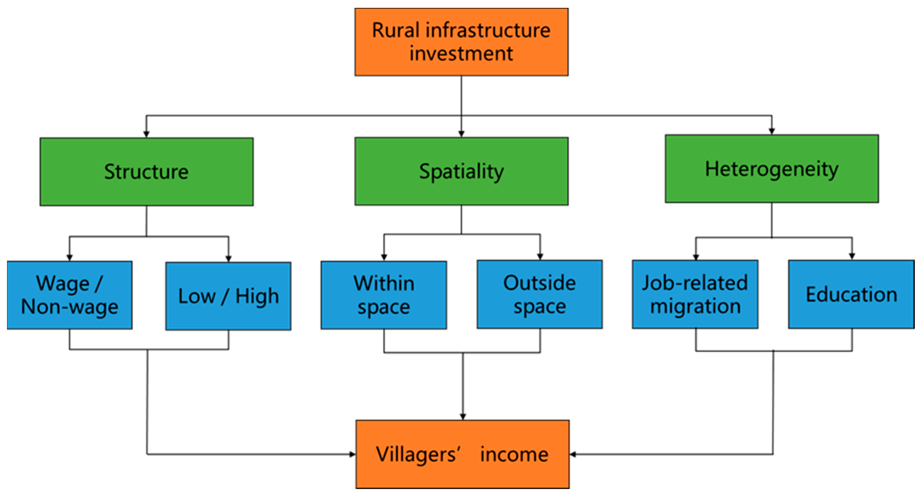
2.1. Theoretical Analysis and Research Hypotheses

2.1.1. Structure of RII

The structural differences in the income-increasing effect of RII mainly lie between wage and non-wage incomes and between high-income and low-income villagers. On the one hand, RII has different mechanisms of action regarding villagers’ wage and non-wage incomes. In response to wage income, LII enhances villagers’ welfare and entrepreneurial basis mainly through indirect effects. LII reduces the mobility and information exchange costs for villagers, alleviates the friction in the job market, and makes it easier for more villagers to go out to work. LII stimulates the development of new local rural industries, where villagers can be matched with suitable jobs without having to travel far from home [36,37]. Industries derived from LII encompass secondary and tertiary industries, such as logistics, packaging, processing, and tourism services, which further increase villagers’ wage income [38]. PII reduces the amount of time villagers spend on agriculture labor, providing more off-farm employment opportunities and increasing wage income. In response to non-wage income, LII and PII have increased villagers’ property income, such as house rent and rent from the transfer of land management rights. PII directly serves as an input factor for agricultural production, increasing agricultural output [39]. PII has facilitated the use of data, agricultural technology equipment, etc. in agricultural production and management, further increasing operating income [40]. Rural areas with good living infrastructure conditions are more likely to attract production subsidies, further increasing transfer income.

On the other hand, who benefits from rural infrastructure, high-income villagers or low-income villagers, is a question worthy of consideration. Rural infrastructure brings more changes in production technology and imposes higher demands on villagers’ initiative. Because there is significant overlap between low-income villagers and those who have difficulty in using technology, RII may be more beneficial to high-income villagers [41]. Generally, high-income villagers are highly educated and enhance their information search and communication abilities through rural infrastructure, thereby enjoying the benefits of rural infrastructure to a greater extent. However, because of the limitations of their education, low-income villagers frequently find it challenging to utilize technical rural infrastructure to develop production or find non-agricultural jobs [30]. Low-income villagers are unable to enhance the scientific nature of production decisions and expand the value chain [42]. Therefore, high-income villagers extract more resources with the assistance of rural infrastructure, thereby forming a Matthew effect of “the rich get richer”.

Hypothesis 1. 

RII increases villagers’ income, but there are disparities in the impacts of LII and PII on villagers’ wage and non-wage incomes, as well as on high-income and low-income villagers.

2.1.2. Spatiality of RII

Villagers’ income tends to be spatially distributed. Low-income rural populations are concentrated in remote rural areas, having strong spatial correlations with the level of rural public goods provision, resource endowments, and other factors. Poor location conditions and backward infrastructure result in weak industry-led capacity, and under the cumulative effect of this non-linear negative cycle, a spatial low-income trap is formed. At the micro level, the difficulty in increasing villagers’ income is the outcome of a combination of the villagers’ endowment and geographical endowment [43]; at the macro level, the difficulty in increasing villagers’ income is a state of dysfunctional coupling among the dimensions of the people, industry, and land within a given space and time. With the advancement of time, villagers are no longer isolated spatially. They are gradually integrated into the marketization process and move freely between urban and rural areas. This movement constitutes an important way for villagers to eliminate poverty. The urbanization process has rendered villagers’ livelihoods as increasingly dependent on non-agricultural industries. Villagers’ consumption patterns, identities, and social mobility have gradually become more in alignment with those of cities. The economy and ecology have broken through the original spatial limitations, and the intensity, complexity, and diversity of connections have increased [44].

Rural infrastructure creates opportunities that no longer rely on local systems for services or livelihoods but can be sourced to more distant geographical areas [45]. Infrastructure, such as rural roads, integrates labor markets across space and enhances the mobility of villagers [46]. The scale and structural characteristics of fiscal expenditure among governments exhibit clear degrees of mutual imitation and strategic interaction. Provinces with better rural infrastructure development prompt neighboring provinces to follow suit [47]. RII in the region expands the scope and efficiency of agricultural product transactions in adjacent areas and brings larger trading markets to adjacent areas. As a result, RII boosts villagers’ income growth. The effect of rural infrastructure on increasing villagers’ income is converging, resulting in spatial correlation in rural infrastructure, namely, the spatial spillover effect.

Hypothesis 2. 

RII exerts a spatial spillover effect on increasing villagers’ income.

2.1.3. Heterogeneity of RII

The essence of rural labor transfer is the choice made after comparing the economic interests of different sectors and those of urban and rural public services. In urban areas, the combination of superior educational resources, convenient transportation, and information networks creates a good environment for residents to participate in higher-quality education or skills training. Coupled with the significant disparity between non-agricultural and agricultural incomes, a large number of rural populations have been attracted. Because of the job-related migration of rural labor, the hollowing out of some rural populations is inevitable [48]. A large number of “empty houses” have emerged in rural areas. A large amount of money has been invested in rural infrastructure construction, which is facing the problem of “for whom it is built”. In areas where the degree of job-related migration is high, the marginal effect of increased income from LII, enjoyed by villagers who go to cities for employment, declines, which weakens the income-increasing effect brought about by LII. PII reduces villagers’ agricultural production costs, enabling villagers to have more time to engage in non-agricultural jobs. In areas with a high degree of job-related migration, the income-increasing effect brought by PII is magnified [49].

Compared with migrant workers in cities, although the number of those who are employed locally or return to their hometowns for employment and entrepreneurship is relatively small, they possess broader academic qualifications and vision and exert a greater role in increasing income through rural infrastructure [50]. The education level of the population has a further influence on the income-increasing effect through its impact on the utilization efficiency of rural infrastructure [51]. In areas with high levels of education, villagers tend to have more employment opportunities, and the income-increasing effect of LII is magnified. However, villagers with higher levels of education are more inclined to work outside their hometowns. Villagers enhance their non-agricultural professional skills through formal education and skills training, thereby driving the growth of their income. In areas with high levels of education, the marginal effect of increased income from PII enjoyed by villagers declines, and the income-increasing effect of PII is diminished.

Hypothesis 3. 

Job-related migration and education levels have moderating effects on the income-increasing effect of RII.

Based on the above theoretical analysis and deduction, this paper constructed a theoretical framework of the multidimensional impact of RII on villagers’ income (Figure 1).

2.2. Variables

• Explained variables. This study employed villagers’ income, wage income, and non-wage income in each province as explained variables. Villagers’ income is the sum of the wage income and non-wage income. Non-wage income comprised villagers’ business income, transfer income, and property income;
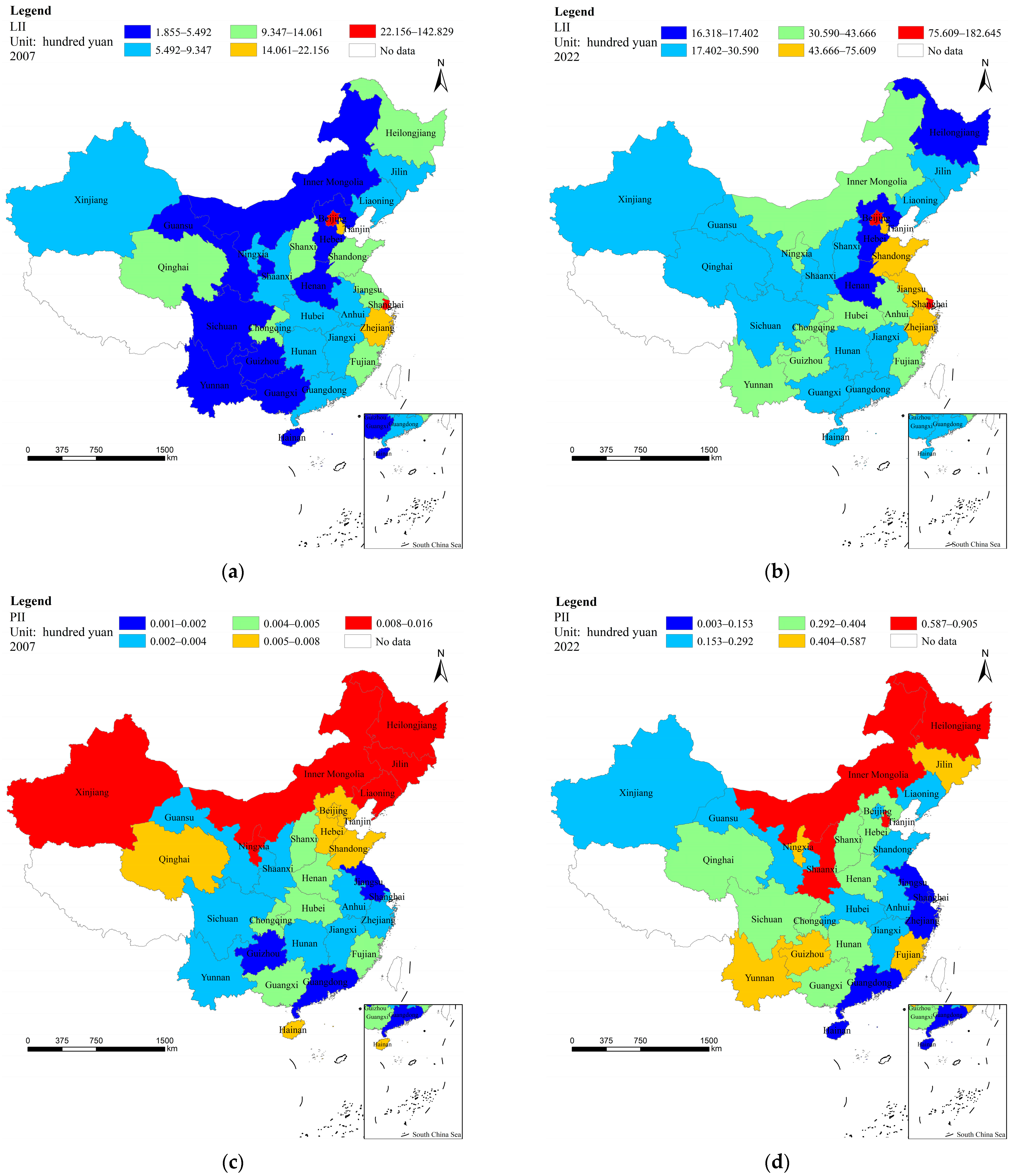
• Explanatory variables. This study categorized rural infrastructure into LII and PII. LII pertained to infrastructure investment in water, gas, heating, roads, drainage, landscaping, environmental sanitation, etc. in rural areas; PII referred to agricultural production construction projects, such as agriculture, forestry and pasture, the purchase of machinery and equipment for agricultural production, as well as investment in farmland construction projects, irrigation, drainage, and other small-scale water conservancy projects in rural townships, villages, and groups. The perpetual inventory method was utilized to calculate RII, and the formula is as follows:

  $$K_t=I_t+(1-{\delta }_t)K_{t-1}$$

  (1)

  In the formula, $K_t$ is the current stock of rural infrastructure fixed capital, $I_t$ is the RII in year $t$ at comparable prices, and ${\delta }_t$ is the depreciation rate, which was 9.6% based on the depreciation convention of rural infrastructure [52];
• Control variables. In addition to the two core explanatory variables of LII and PII, this study employed control variables, such as the job-related migration level, education level, economic development level, urbanization level, cultivated land endowment, openness level, and agricultural development level, referring to the practices of the existing literature [10,53,54]. The job-related migration level was expressed as the proportion of migrant laborers to aggregate laborers; the education level was expressed as the average number of years of the villagers’ education; the economic development level was expressed as the per capita comparable gross domestic product (GDP); the urbanization level was expressed as the urbanization rate; the cultivated land endowment was expressed as the ratio of the family-operated cultivated land area to the number of people in the rural population; the openness level was expressed as the proportion of the total import and export volume to the GDP; the agricultural development level was expressed as the proportion of the gross agricultural production to the GDP.

To eliminate the factor of inflation, all the variables related to currency, designed in this study, have been converted to the comparable prices of 2007.

2.3. Data

The data of this study were the panel data of 30 provinces in inland China, except for Tibet, from 2007 to 2022. The data came from the annual China Urban and Rural Construction Statistical Yearbook [55], China Statistical Yearbook [56], China Population and Employment Statistical Yearbook [57], and China Rural Policy and Reform Statistical Bulletin [58]. The descriptive statistics of each variable are shown in

Table 1. Variable definitions and descriptive statistics.

	Variable Name	Variable Code	Meaning (Unit)	Average Value	Standard Deviation	Minimum	Maximum
Explained variables	Villagers’ income	$y$	Per capita income of villagers (Ten thousand yuan)	0.953	0.465	0.252	2.726
	Villagers’ wage income	$y^w$	Per capita wage income of villagers (Ten thousand yuan)	0.418	0.337	0.039	1.779
	Villagers’ non-wage income	$y^n$	Per capita non-wage income of villagers (Ten thousand yuan)	0.535	0.205	0.167	1.124
Explanatory variables	LII	$k^l$	Per capita LII (yuan)	2523.900	3217.100	185.595	18,807.080
	PII	$k^p$	Per capita PII (yuan)	1.560	1.354	0.113	8.573
Control variables	Job-related migration level	$lab$	Number of migrant laborers/aggregate laborers (%)	31.440	9.480	6.470	54.890
	Education level	$edu$	Average number of years of education for rural population (years)	7.779	0.650	5.878	10.118
	Economic development level	$pgdp$	Per capita GDP (Ten thousand yuan)	3.608	2.039	0.538	11.932
	Urbanization level	$urb$	Urbanization rate (%)	58.182	13.039	29.110	89.600
	Cultivated land endowment	$land$	Area of cultivated land managed by households/number of people in rural population (mu *)	2.733	2.156	0.162	13.756
	Openness level	$open$	Total import and export volume/GDP (%)	26.488	28.088	0.715	154.937
	Agricultural development level	$agr$	Gross agricultural production/GDP (%)	12.436	6.933	0.280	41.530

* 1 mu = 1/15 ha.

.

2.4. Methods

• Standard Deviational Ellipse (SDE) Model. The SDE model is a statistical method used to describe the spatial directional characteristics of economic geographical elements. In this study, the SDE model was employed to depict the changing trajectories and discrete trends of the centers of gravity of RII and villagers’ income in China. The specific calculation formulae are as follows:

  $$\left\{\begin{array}{l}\overline{x}={\displaystyle \sum _{i=1}^n{w}_i{x}_i}/{\displaystyle \sum _{i=1}^n{w}_i}\\ \overline{y}={\displaystyle \sum _{i=1}^n{w}_i{y}_i}/{\displaystyle \sum _{i=1}^n{w}_i}\end{array}\right.$$

  (2)

  $$\tan \theta =\left[\left({\displaystyle \sum _{i=1}^n{w}_i^2{x}_i^2-{\displaystyle \sum _{i=1}^n{w}_i^2{y}_i^2}}\right)+\sqrt{{\left({\displaystyle \sum _{i=1}^n{w}_i^2{x}_i^2-{\displaystyle \sum _{i=1}^n{w}_i^2{y}_i^2}}\right)}^2+4{\left({\displaystyle \sum _{i=1}^n{w}_i^2{x}_i^2{y}_i^2}\right)}^2}\right]/{\displaystyle \sum _{i=1}^{n}2w_i^2{x}_i{y}_i}$$

  (3)

  $$\left\{\begin{array}{l}{\sigma }_x=\sqrt{2{\displaystyle \sum _{i=1}^n{(w_i{x}_i\cos \theta -w_i{y}_i\sin \theta )}^2/{\displaystyle \sum _{i=1}^n{w}_i^2}}}\\ {\sigma }_y=\sqrt{2{\displaystyle \sum _{i=1}^n{(w_i{x}_i\sin \theta -w_i{y}_i\cos \theta )}^2/{\displaystyle \sum _{i=1}^n{w}_i^2}}}\end{array}\right.$$

  (4)

  $$S=\pi {\sigma }_x{\sigma }_y$$

  (5)

  $$f={\displaystyle \frac{{\sigma }_x-{\sigma }_y}{{\sigma }_x}}$$

  (6)

  where $\left(\overline{x},\overline{y}\right)$ is the central coordinate; $\left(x_i,y_i\right)$ is the particle coordinate of province $i$; $\theta$ is the directional angle of the spatial distribution; ${\sigma }_x$ and ${\sigma }_y$ are the standard deviations of the major and minor axes of the ellipse; $S$ is the area of the ellipse; and $f$ is the oblateness of the ellipse;
• Multiple Regression Model. Considering only the structure of the villagers’ wage income and non-wage income, as well as the heterogeneity of the job-related migration and education level, the multiple regression model was set as follows:

  $$y_{it}=\alpha +{\beta }_1{k}_{it}^l+{\beta }_2{k}_{it}^p+{\displaystyle \sum _m{\theta }_m}{X}_{mit}+{\epsilon }_{it}$$

  (7)

  where $y_{it}$ represents villagers’ income, including villagers’ wage income ($y_{it}^w$) and non-wage income ($y_{it}^n$); $k_{it}^l$ and $k_{it}^p$ represent LII and PII; $X_{mit}$ represents a series of control variables; ${\epsilon }_{it}$ is the residual term; the subscript $i$ represents the province; the subscript $t$ represents the year; and $\alpha$, $\beta$, and $\theta$ are the corresponding variable coefficients. This study employed a fixed effect model. To eliminate possible endogenous effects, the core explanatory variables were lagged by one period;
• Quantile regression model. The quantile regression model compares the influence of the independent variable on the dependent variable at different quantile points [59]. When the explanatory variable has varying effects on the explained variable at different quantiles, such as left skewness or right skewness, quantile regression captures the tail characteristics of the distribution. It was utilized to examine the differences in the income-increasing effect of RII between high-income villagers and low-income villagers. For a population of random variables ($y$), the general linear conditional quantile function for the τth quantile is as follows:

  $$Q(\tau |X=x)=x^{\prime }\beta (\tau )$$

  (8)
  For any $\tau \in (0,1)$, $x_i$ is a p-dimensional vector, ${\rho }_{\tau }(·)$ is the tilted absolute value function, and the estimated value $\widehat{\beta }(\tau )$ shown in the following formula is called the regression coefficient estimate at the τth quantile:

  $$\widehat{\beta }(\tau )=argmi{n}_{\beta \in R^P}{\displaystyle \sum _{i=1}^n{\rho }_{\tau }(y_i-x_i^{\prime }\beta )}$$

  (9)
• Spatial panel regression model. The spatial panel regression model includes the spatial autoregression model (SAR), the spatial Durbin model (SDM), and the spatial error model (SEM). They were used to consider the spatial spillover effect of RII. The general expressions are as follows:

  $$\mathrm{SAR}:y_{it}=\lambda W{y}_{it}+{\beta }_1{k}_{it}^l+{\beta }_2{k}_{it}^p+{\displaystyle \sum _m{\theta }_m}{X}_{mit}+{\epsilon }_{it}$$

  (10)

  $$\mathrm{SDM}:y_{it}={\beta }_1{k}_{it}^l+{\beta }_2{k}_{it}^p+{\displaystyle \sum _m{\theta }_m}{X}_{mit}+{\beta }_{3}W{k}_{it}^l+{\beta }_{4}W{k}_{it}^p+{\displaystyle \sum _n{\delta }_n}W{X}_{nit}+{\epsilon }_{it}$$

  (11)

  $$\mathrm{SEM}:\left\{\begin{array}{l}{y}_{it}={\beta }_1{k}_{it}^l+{\beta }_2{k}_{it}^p+{\displaystyle \sum _m{\theta }_m}{X}_{mit}+u_{it}\\ u_{it}=\rho W{u}_{it}+{\epsilon }_{it},{\epsilon }_{it}\sim N(0,{\sigma }^2{I}_n)\end{array}\right.$$

  (12)

  where $y_{it}$ represents villagers’ income; $k_{it}^l$ and $k_{it}^p$ represent LII and PII; $X_{mit}$ represents a series of control variables; $W$ is the spatial weight matrix (the spatial weight matrix used in this study was the adjacency matrix); $\lambda$, $\delta$ and, $\rho$ are the corresponding spatial regression coefficients; $\beta$ and $\theta$ are the corresponding variable coefficients; $\epsilon$ is the random error term; and $u$ is the disturbance term.

In the above content, the SDE model was mainly used to describe the current situation of RII and villagers’ income, presenting an intuitive perception. The multiple regression model was used first to verify the different effects of RII on wage income and non-wage income in Hypothesis 1 and then to conduct regression based on the grouping situations of job-related migration and the education level to verify Hypothesis 3. The quantile regression model was used to verify the different effects of RII on the high-income group and the low-income group in Hypothesis 1. The spatial panel regression model was used to verify the spatial effect of RII in Hypothesis 2.

3. Results and Discussion

3.1. Analysis of Spatial Agglomeration Characteristics

3.1.1. Spatial Static Distribution

In order to explore the spatial distributions of the rural infrastructure and villagers’ income, this study selected two years, 2007 and 2022, and divided the variables into five categories using the natural breakpoint method. As can be seen from Figure 2a,b, regions in China with less LII presented a clear agglomeration pattern. In 2007, regions with less LII were concentrated in the southwest region of China and provinces such as Gansu, Inner Mongolia, Hebei, and Henan. In 2022, provinces with less LII were concentrated in Hebei, Henan, and Heilongjiang. As can be seen from Figure 2c,d, regions in China with more PII presented a clear agglomeration pattern. In 2007, regions with more PII were concentrated in northern provinces, such as Heilongjiang, Jilin, Liaoning, Inner Mongolia, and Xinjiang. In 2022, regions with more PII were concentrated in northern provinces, such as Heilongjiang, Inner Mongolia, and Shaanxi. As can be seen from Figure 2e,f, villagers’ income presented a clear agglomeration pattern. In 2007 and 2022, provinces with higher villagers’ incomes were concentrated in China’s eastern coastal areas, while provinces with lower villagers’ incomes were concentrated in the western regions of China.

3.1.2. Spatial Dynamic Distribution

Through the calculations of the SDE model, it can be seen from Figure 3 and

Table 2. Results of standard deviational ellipse correlation parameters.

Variable Name	Year	Area (Ten Thousand km2)	Center Point Coordinates	Minor Axis (km)	Major Axis (km)	Flattening (Unitless)	Declination (°)
LII	2007	249.969	115°54′ E, 35°28′ N	871.350	913.152	0.046	170.098
	2015	265.890	114° 37′ E, 35°5′ N	849.830	995.910	0.147	22.455
	2022	299.524	113°52′ E, 4°15′ N	913.901	1043.236	0.124	31.304
PII	2007	467.778	112°24′ E, 37°1′ N	1335.249	1115.135	0.165	51.183
	2015	365.961	112°53′ E, 36°52′ N	948.408	1228.257	0.228	40.147
	2022	431.703	112°21′ E, 35°39′ N	1126.123	1220.251	0.077	44.408
Villagers’ income	2007	333.213	113°41′ E, 33°44′ N	946.037	1121.150	0.156	22.577
	2015	337.494	113°52′ E, 33°51′ N	950.696	1129.989	0.159	24.812
	2022	339.613	114°12′ E, 33°58′ N	960.270	1125.747	0.147	24.769

, from 2007 to 2022, the focus of LII gradually shifted from the northeast to the southwest. The flattened standard deviational ellipse first presented a significant increase and then slightly decreased, indicating that the concentration of China’s LII in the “northeast–southwest” direction increased and then slightly weakened. The area of the standard deviational ellipse has continuously increased, indicating that the scope of LII in China has continued to expand. The focus of PII shifted from the northwest to the southeast and then from the northeast to the southwest. The flatness of the standard deviational ellipse first increased and then decreased. The focus of LII in the “northeast–southwest” direction in China increased and then weakened. The area of the standard deviational ellipse first increased and then decreased, indicating that the scope of PII first increased and then weakened. The focus of villagers’ income gradually shifted from the northeast to the southwest, and the flatness of the standard deviational ellipse first increased and then decreased, which was consistent with the change directions of LII and PII, indicating that villagers’ income had an obvious spatial correlation with RII.

3.2. Results of Structure

Through the calculations of the multiple regression model, the results of the disparities between wage and non-wage incomes were obtained, as shown in

Table 3. Results of the disparities between wage and non-wage incomes.

Variable Name	Villagers’ Income	Villagers’ Wage Income	Villagers’ Non-Wage Income
$k^l$	4 × 10−5 *** (8 × 10−6)	5 × 10−5 *** (6 × 10−6)	−8 × 10−6 (5 × 10−6)
$k^p$	0.046 *** (0.008)	0.019 *** (0.006)	0.027 *** (0.005)
$lab$	0.004 ** (0.002)	0.003 ** (0.001)	0.001 (0.001)
$edu$	0.127 *** (0.026)	0.071 *** (0.019)	0.056 *** (0.010)
$pgdp$	0.110 *** (0.010)	0.055 *** (0.008)	0.055 *** (0.007)
$urb$	0.013 *** (0.002)	0.003 ** (0.002)	0.010 *** (0.001)
$land$	−0.020 ** (0.009)	−0.051 *** (0.007)	0.031 *** (0.006)
$open$	−0.005 *** (0.001)	−0.004 *** (0.001)	−0.001 (0.001)
$agr$	0.005 ** (0.003)	0.007 *** (0.002)	−0.002 (0.002)
_cons	−1.387 *** (0.208)	−0.607 *** (0.154)	−0.780 *** (0.136)
	F(9, 411) = 575.25 ***	F(9, 411) = 245.27 ***	F(9, 411) = 403.84 ***

Note: ***/** indicate significance at the 1%/5% levels.

; it can be observed that both LII and PII have a significant income-increasing effect. For every 1-yuan increase in LII, villagers’ income increased by 0.004%, and for every 1-yuan increase in PII, villagers’ income increased by 4.6%. From the perspective of income decomposition, both LII and PII had an increasing effect on wage income, and PII had an increasing effect on non-wage income, but the increasing effect of LII on non-wage income was not significant. The levels of job-related migration and agricultural development had significant positive effects on villagers’ income and wage income. The possible reason was that in provinces with a higher level of agricultural development, agricultural competition was more intense, and more people chose to work outside these provinces. At the same time, migrant workers had more non-agricultural employment opportunities. The levels of education, economic development, and urbanization had significant positive effects on villagers’ income, wage income, and non-wage income, indicating that the higher the levels of education, economic development, and urbanization, the higher the villagers’ income. Cultivated land endowment had significant negative effects on villagers’ income and wage income but had a significant positive effect on non-wage income, indicating that regions with better cultivated land endowments increased the opportunity cost of villagers working outside the home while bringing more favorable conditions for agricultural production, reducing villagers’ wage income, and increasing villagers’ non-wage income. The level of openness to the outside world had significant negative effects on villagers’ income and wage income. A possible reason is that the higher the degree of openness, the more intense the employment competition, which was not conducive to increase villagers’ wage income in that region, thereby verifying Hypothesis 1: RII increases villagers’ income, but there are disparities in the impacts of LII and PII on villagers’ wage and non-wage incomes.

This study employed the quantile regression method to analyze the differential impacts of RII on villagers with different income levels and selected five quantiles of 10%, 25%, 50%, 75%, and 90%, respectively representing the low-income group, the lower-middle-income group, the middle-income group, the higher-middle-income group, and the high-income group.

Table 4. Results of the disparities between high-income and low-income groups.

Variable Name	Villagers’ Income	Villagers’ Wage Income	Villagers’ Non-Wage Income
10% quantile
$k^l$	2 × 10−5 (2 × 10−5)	4 × 10−5 ** (2 × 10−5)	−9 × 10−6 (1 × 10−5)
$k^p$	0.025 (0.022)	0.012 (0.013)	0.015 (0.013)
25% quantile
$k^l$	3 × 10−5 * (2 × 10−5)	4 × 10−5 *** (1 × 10−5)	−8 × 10−6 (1 × 10−5)
$k^p$	0.033 ** (0.017)	0.015 (0.009)	0.020 ** (0.009)
50% quantile
$k^l$	4 × 10−5 *** (1 × 10−5)	5 × 10−5 *** (8 × 10−6)	−8 × 10−6 (8 × 10−6)
$k^p$	0.046 *** (0.012)	0.019 *** (0.006)	0.027 *** (0.007)
75% quantile
$k^l$	5 × 10−5 *** (1 × 10−5)	6 × 10−5 *** (1 × 10−5)	−7 × 10−6 (1 × 10−5)
$k^p$	0.058 *** (0.015)	0.024 *** (0.008)	0.034 *** (0.011)
90% quantile
$k^l$	7 × 10−5 *** (2 × 10−5)	6 × 10−5 *** (1 × 10−5)	−7 × 10−6 (2 × 10−5)
$k^p$	0.068 *** (0.022)	0.026 ** (0.011)	0.039 *** (0.001)
Control variables are controlled.

Note: ***/**/* indicate significance at the 1%/5%/10% levels.

presents the results of the quantile regression.

From the quantile regression results in Table 4, it is observed that at the quantile levels ranging from 25% to 90%, both LII and PII had an effect on increasing villagers’ income. Further comparison of the regression coefficients indicated that as the percentile of villagers’ income levels rose, the marginal effects of LII and PII on villagers’ income demonstrated an upward trend. From the lower-middle-income groups to the high-income groups, for every unit of increase in LII, the growth trend of villagers’ income levels was 0.003%→0.004%→0.005%→0.007%, and for every unit of increase in PII, the growth trend of villagers’ income levels was 3.30%→4.64%→5.76%→6.81%, suggesting that RII would be more beneficial to high-income villagers, thereby verifying Hypothesis 1: RII increases villagers’ income, but there are disparities in the impacts of LII and PII on high-income and low-income villagers.

3.3. Results of Spatiality

This study employed the SAR, SEM, and SDM to estimate and compare the samples. First, the optimal spatial econometric model needed to be determined. The estimation strategy adopted in this study was to conduct likelihood ratio (LR) tests and Akaike information criterion tests (AIC). The relevant test results are presented in

Table 5. Correlation test results of the spatial econometric model.

Related Tests	Value	p-Value
LR test (SDM degenerates to SEM)	376.85	0.000
LR test (SDM degenerates to SAR)	262.23	0.000
AIC value of SDM	−1101.865	-
AIC value of SEM	−743.017	-
AIC value of SAR	−857.632	-
Hausman test	17.76	0.038

. The LR tests indicated that the SDM cannot be degenerated into the SEM model and the SAR model, so the SDM was utilized. The AIC tests also revealed that the SDM was optimal. After the Hausman test, the results supported the use of the fixed effect model, so this study employed the fixed effect model for the analysis.

This study decomposed the total spatial effect of RII on villagers’ income into the direct effect and the indirect effect. The direct effect was employed to capture the impacts of influencing factors on the region, and the indirect effect was employed to capture the impacts on neighboring regions. As can be seen from

Table 6. Spatial econometric analysis results.

Variable Name	Direct Effect	Indirect Effect	Total Effect
$k^l$	4 × 10−5 *** (5 × 10−6)	6 × 10−5 *** (1 × 10−5)	1 × 10−4 *** (1 × 10−5)
$k^p$	−0.011 ** (0.005)	0.035 *** (0.012)	0.024 * (0.013)
$lab$	−0.004 *** (0.001)	0.017 *** (0.003)	0.013 *** (0.003)
$edu$	0.011 (0.016)	0.028 (0.037)	0.039 (0.043)
$pgdp$	0.071 *** (0.007)	−0.042 *** (0.016)	0.029 (0.019)
$urb$	−0.008 *** (0.002)	0.024 *** (0.003)	0.016 *** (0.003)
$land$	−0.025 *** (0.007)	0.048 *** (0.013)	0.023 (0.016)
$open$	0.001 (0.001)	−0.002 * (0.001)	−0.002 (0.001)
$agr$	0.006 *** (0.002)	−0.020 *** (0.004)	−0.015 *** (0.005)
Rho	0.289 *** (0.049)	Log-likelihood	684.616

Note: ***/**/* indicate significance at the 1%/5%/10% levels.

, the impacts of LII and PII on villagers’ income presented a positive total effect. LII and PII not only exerted the income-increasing effect on villagers in the local area but also exerted the spatial spillover effect. For every 1-yuan increase in LII, villagers’ income in neighboring areas increased by 0.006%, and for every 1-yuan increase in PII, villagers’ income in neighboring areas increased by 3.52%. From the perspective of effect decomposition, the indirect effect brought about by RII was stronger than the direct effect, thereby verifying Hypothesis 2: RII exerts a spatial spillover effect on increasing villagers’ income.

3.4. Results of Heterogeneity

This study employed the national average as the line to divide provinces into those with low and high levels of job-related migration and those with low and high levels of education. As can be seen from

Table 7. Heterogeneous impacts of job-related migration and education.

Variable Name	Low Level of Job-Related Migration	High Level of Job-Related Migration	Low Level of Education	High Level of Education
$k^l$	5 × 10−5 *** (1 × 10−5)	−2 × 10−6 (1 × 10−5)	1 × 10−5 (1 × 10−5)	4 × 10−5 *** (1 × 10−5)
$k^p$	0.037 *** (0.011)	0.041 *** (0.008)	0.084 *** (0.010)	0.032 *** (0.011)
$lab$	-	-	−0.002 (0.002)	0.010 *** (0.003)
$edu$	0.193 *** (0.036)	0.018 (0.026)	-	-
$pgdp$	0.096 *** (0.014)	0.135 *** (0.013)	0.084 *** (0.013)	0.136 *** (0.014)
$urb$	0.026 *** (0.003)	0.015 *** (0.002)	0.020 *** (0.002)	0.020 *** (0.004)
$land$	−0.029 ** (0.013)	−0.002 (0.011)	−0.018 * (0.009)	−0.145 *** (0.040)
$open$	−0.006 *** (0.001)	2 × 10−4 (0.001)	0.003 *** (0.001)	−0.004 *** (0.001)
$agr$	0.020 *** (0.004)	−0.001 (0.002)	−0.001 (0.003)	0.003 (0.004)
_cons	−2.668 *** (0.331)	−0.550 *** (0.200)	−0.599 *** (0.110)	−0.803 *** (0.220)
	F(8, 188) = 294.53 ***	F(8, 216) = 703.06 ***	F(8, 216) = 516.32 ***	F(8, 188) = 310.17 ***

Note: ***/**/* indicate significance at the 1%/5%/10% levels.

, in provinces with low job-related migration levels, for every 1-yuan increase in LII, villagers’ income increased by 0.005%, and for every 1-yuan increase in PII, villagers’ income increased by 3.72%; in provinces with high job-related migration levels, the income-increasing effect of LII was insignificant. For every 1-yuan increase in PII, villagers’ income increased by 4.14%. This indicated that the increase in the level of job-related migration had suppressed the income-increasing effect of LII but promoted the income-increasing effect of PII. In provinces with high levels of education, for every 1-yuan increase in LII, villagers’ income increased by 0.004%, and for every 1-yuan increase in PII, villagers’ income increased by 3.15%; in provinces with low levels of education, the income-increasing effect of LII was insignificant. For every 1-yuan increase in PII, villagers’ income increased by 8.35%. This indicated that the improvement of the education level has promoted the income-increasing effect of LII but inhibited the income-increasing effect of PII, thereby verifying Hypothesis 3: Job-related migration and education levels have moderating effects on the income-increasing effect of RII.

3.5. Discussion

In the context of developing countries achieving sustainable development goals, the exploration of the income-increasing effect of RII is crucial for increasing villagers’ income and achieving common prosperity. This study has placed the structure, spatiality, and heterogeneity of RII in the same analytical framework. By calculating the value of RII, it has comprehensively examined the impact of RII on villagers’ income, which is of great significance for reference for developing countries to formulate RII policies and increase the income of villagers. The research results show that first, RII has an income-increasing effect. This view is verified by previous studies [60] and has been confirmed in low- and middle-income countries [42]. In this study, RII is further divided into LII and PII, and income is divided into wage income and non-wage income or into high income and low income for regression. The regression results are consistent with those of previous studies [61]. The same research results also exist in South Africa [62]. Among them, the subtle difference is that the effect of LII on non-wage income is not obvious. The main reason for this is that except for roads and communication facilities, which have dual attributes of production and life in LII [42], the correlations between other infrastructures and non-wage income are not significant. Second, RII exerts a spatial spillover effect on increasing villagers’ income, which is consistent with the results of previous studies [63]; this spatial spillover effect also exists in the Belt-and-Road-Initiative countries [64]. Third, job-related migration and education levels have moderating effects on the income-increasing effect of RII. This is supported by previous studies [21,65].

4. Conclusions

This study estimated the capital stock of China’s provincial RII from 2007 to 2022 based on the perpetual stock method and analyzed the income-increasing effect of RII from the three-dimensional perspectives of structure, spatiality, and heterogeneity. The conclusions show that (1) in terms of structure, both LII and PII promote wage income. PII has an increasing effect on non-wage income, but the increasing effect of LII on non-wage income is not evident. Meanwhile, the income-increasing effect of RII for high-income groups is larger than that for low-income groups. (2) In terms of spatiality, RII has a spatial spillover effect, which increases villagers’ income in neighboring areas. From the perspective of spatial effect decomposition, the indirect effect of RII even exceeds the direct effect. (3) In terms of heterogeneity, an increase in the level of job-related migration inhibits the income-increasing effect of LII but promotes the income-increasing effect of PII; the improvement of the education level promotes the income-increasing effect of LII but inhibits the income-increasing effect of PII.

Because the income-increasing effect of RII has structural, spatial, and heterogeneous influences, developing countries take the following into consideration when formulating and implementing policies to strengthen RII and increase villagers’ income: (1) Given that the income-increasing effect of RII on high-income villagers is greater than that on low-income villagers, support and assistance to vulnerable groups in rural areas should be enhanced; more inclusive and equitable sustainable development strategies should be adopted; education coverage and non-agricultural employment training for vulnerable groups in rural areas should be strengthened; the driving effect brought about by RII should be expanded, and opportunities for vulnerable groups to share the dividends of rural infrastructure construction should be increased. (2) Given the spatial nature of RII, in China, villagers in economically underdeveloped areas rely more on non-wage income, but the role of LII in promoting non-wage income is not obvious, indicating that LII in underdeveloped areas is still lagging. The regional layout of rural infrastructure should be optimized by the government. RII should be focused on underdeveloped areas. The shortcomings of rural infrastructure should be targeted. The focus and timing of rural infrastructure construction should be determined in accordance with local conditions based on regional, human, financial, material, and other factors to promote the coordinated development of rural infrastructure in that region and neighboring areas. (3) Given that both job-related migration and education levels have impacts on the income-increasing effect of RII, urban and rural population mobilities and differences in education levels should be taken into account. The development positioning of villages should be reasonably determined. RII should be promoted to adapt to changes in rural job-related migration and education levels. The problem of “for whom and by whom” rural infrastructure is built should be solved.

Some limitations of this study lie in the fact that it relies on China’s macroeconomic indicators and calculates based on provinces as units, resulting in the averaging of RII. It seems reasonable to conduct regressions on smaller administrative units, such as county-level administrative units, which can better demonstrate the differences in RII investments. Therefore, in subsequent studies, on the one hand, we plan to conduct research within smaller administrative units, such as county-level or municipality-level units, to reduce the error in averaging RII; on the other hand, based on the microdata of farmers, we will study the changes in farmers’ behaviors and incomes before and after the implementation of RII.

References

1. The General Office of the Central Committee of the Communist Party of China and the General Office of the State Council Have Jointly Issued the “Implementation Plan for Rural Construction Actions”. Available online: https://www.gov.cn/zhengce/2022-05/23/content_5691881.htm (accessed on 4 December 2024).
2. The Investment Scale for Rural Vitalization Will Exceed 7 Trillion Yuan. Available online: http://finance.people.com.cn/n1/2019/0121/c1004-30579935.html (accessed on 4 December 2024).
3. By 2030, China Will Have Built 1.2 Billion Mu of High-Standard Farmland and Renovated and Upgraded 280 Million Mu. Available online: https://www.gov.cn/zhengce/2021-09/17/content_5637900.htm (accessed on 4 December 2024).
4. Zhou, F.; Guo, X.; Liu, C.; Ma, Q.; Guo, S. Analysis on the influencing factors of rural infrastructure in China. Agriculture 2023, 13, 986. [Google Scholar] [CrossRef]
5. Qin, X.; Wu, H.; Shan, T. Rural infrastructure and poverty in China. PLoS ONE 2022, 17, e0266528. [Google Scholar] [CrossRef] [PubMed]
6. In 2023, Residents’ Income Achieved Restorative Growth, and the Gap between Urban and Rural Areas Continued to Narrow. Available online: https://news.cctv.com/2024/01/26/ARTIwZoF6nFiPgc6jG63nZkY240126.shtml (accessed on 9 December 2024).
7. Haberler, G. The place of the General Theory of Employment, Interest, and Money in the history of economic thought. Rev. Econ. Stat. 1946, 28, 187–194. [Google Scholar] [CrossRef]
8. Chakamera, C.; Alagidede, P. The nexus between infrastructure (quantity and quality) and economic growth in Sub Saharan Africa. Int. Rev. Econ. 2018, 32, 641–672. [Google Scholar] [CrossRef]
9. Dah, O.; Bassolet, T.B. Agricultural infrastructure public financing towards rural poverty alleviation: Evidence from West African Economic and Monetary Union (WAEMU) States. SN Bus. Econ. 2021, 1, 39. [Google Scholar] [CrossRef]
10. Chotia, V.; Rao, N. Investigating the interlinkages between infrastructure development, poverty and rural–urban income inequality: Evidence from BRICS nations. Stud. Econ. Financ. 2017, 34, 466–484. [Google Scholar] [CrossRef]
11. Hulten, C.R.; Bennathan, E.; Srinivasan, S. Infrastructure, externalities, and economic development: A study of the Indian manufacturing industry. World Bank Econ. Rev. 2006, 20, 291–308. [Google Scholar] [CrossRef]
12. Akbar, M.; Abdullah; Naveed, A.; Syed, S.H. Does an improvement in rural infrastructure contribute to alleviate poverty in Pakistan? A spatial econometric analysis. Soc. Indic. Res. 2022, 162, 475–499. [Google Scholar] [CrossRef]
13. Ogun, T.P. Infrastructure and poverty reduction: Implications for urban development in Nigeria. In Proceedings of the Urban Forum, Rio de Janeiro, Brazil, 22–26 March 2010; pp. 249–266. [Google Scholar]
14. Zhang, L.; Zhuang, Y.; Ding, Y.; Liu, Z. Infrastructure and poverty reduction: Assessing the dynamic impact of Chinese infrastructure investment in sub-Saharan Africa. J. Asian Econ. 2023, 84, 101573. [Google Scholar] [CrossRef]
15. Sewell, S.J.; Desai, S.A.; Mutsaa, E.; Lottering, R.T. A comparative study of community perceptions regarding the role of roads as a poverty alleviation strategy in rural areas. J. Rural Stud. 2019, 71, 73–84. [Google Scholar] [CrossRef]
16. Oisasoje, O.M.; Ojeifo, S.A. The role of public infrastructure in poverty reduction in the rural areas of Edo State, Nigeria. Res. Humanit. Soc. Sci. 2012, 2, 109–120. [Google Scholar]
17. Medeiros, V.; Ribeiro, R.S.M.; do Amaral, P.V.M. Infrastructure and household poverty in Brazil: A regional approach using multilevel models. World Dev. 2021, 137, 105118. [Google Scholar] [CrossRef]
18. Wan, G.; Wang, C.; Zhang, X.; Zuo, C. Income inequality effect of public utility infrastructure: Evidence from rural China. World Dev. 2024, 179, 106594. [Google Scholar] [CrossRef]
19. Liu, X.; Zeng, F. Poverty reduction in China: Does the agricultural products circulation infrastructure matter in rural and urban areas? Agriculture 2022, 12, 1208. [Google Scholar] [CrossRef]
20. Xiao, H.; Zheng, X.; Xie, L. Promoting pro-poor growth through infrastructure investment: Evidence from the Targeted Poverty Alleviation program in China. China Econ. Rev. 2022, 71, 101729. [Google Scholar] [CrossRef]
21. Lu, H.; Zhao, P.; Hu, H.; Zeng, L.; Wu, K.S.; Lv, D. Transport infrastructure and urban-rural income disparity: A municipal-level analysis in China. J. Transp. Geogr. 2022, 99, 103292. [Google Scholar] [CrossRef]
22. Niu, G.; Jin, X.; Wang, Q.; Zhou, Y. Broadband infrastructure and digital financial inclusion in rural China. China Econ. Rev. 2022, 76, 101853. [Google Scholar] [CrossRef]
23. Shijie, J.; Liyin, S.; Li, Z. Empirical study on the contribution of infrastructure to the coordinated development between urban and rural areas: Case study on water supply projects. Procedia Environ. Sci. 2011, 11, 1113–1118. [Google Scholar] [CrossRef]
24. Ansar, A.; Flyvbjerg, B.; Budzier, A.; Lunn, D. Should we build more large dams? The actual costs of hydropower megaproject development. Energy Policy 2014, 69, 43–56. [Google Scholar] [CrossRef]
25. Rhoda, R. Rural development and urban migration: Can we keep them down on the farm? Int. Migr. Rev. 1983, 17, 34–64. [Google Scholar] [CrossRef] [PubMed]
26. Asher, S.; Novosad, P. Rural roads and local economic development. Am. Econ. Rev. 2020, 110, 797–823. [Google Scholar] [CrossRef]
27. Charlery, L.C.; Qaim, M.; Smith-Hall, C. Impact of infrastructure on rural household income and inequality in Nepal. J. Dev. Eff. 2016, 8, 266–286. [Google Scholar] [CrossRef]
28. Huang, R.; Yao, X. The role of power transmission infrastructure in income inequality: Fresh evidence from China. Energy Policy 2023, 177, 113564. [Google Scholar] [CrossRef]
29. Wang, L.; Zhang, F.; Wang, Z.; Tan, Q. The impact of rural infrastructural investment on farmers’ income growth in China. China Agric. Econ. Rev. 2022, 14, 202–219. [Google Scholar] [CrossRef]
30. Barrios, E.B. Infrastructure and rural development: Household perceptions on rural development. Prog. Plan. 2008, 70, 1–44. [Google Scholar] [CrossRef]
31. Jiang, A.; Zhang, Y.; Ao, Y. Constructing inclusive infrastructure evaluation framework—Analysis influence factors on rural infrastructure projects of China. Buildings 2022, 12, 782. [Google Scholar] [CrossRef]
32. Chen, C.; Ao, Y.; Wang, Y.; Li, J. Performance appraisal method for rural infrastructure construction based on public satisfaction. PLoS ONE 2018, 13, e0204563. [Google Scholar] [CrossRef] [PubMed]
33. Shen, L.; Lu, W.; Peng, Y.; Jiang, S. Critical assessment indicators for measuring benefits of rural infrastructure investment in China. J. Infrastruct. Syst. 2011, 17, 176–183. [Google Scholar] [CrossRef]
34. Krakowiak-Bal, A.; Ziemianczyk, U.; Wozniak, A. Building entrepreneurial capacity in rural areas: The use of AHP analysis for infrastructure evaluation. Int. J. Entrep. Behav. Res. 2017, 23, 903–918. [Google Scholar] [CrossRef]
35. Kandilov, I.T.; Renkow, M. Infrastructure investment and rural economic development: An evaluation of USDA’s broadband loan program. Growth Change 2010, 41, 165–191. [Google Scholar] [CrossRef]
36. Shabani, Z.D.; Safaie, S. Do transport infrastructure spillovers matter for economic growth? Evidence on road and railway transport infrastructure in Iranian provinces. Reg. Sci. Policy Pract. 2018, 10, 49–64. [Google Scholar] [CrossRef]
37. Matas, A.; Raymond, J.-L.; Roig, J.-L. Wages and accessibility: The impact of transport infrastructure. Reg. Stud. 2015, 49, 1236–1254. [Google Scholar] [CrossRef]
38. Deller, S.C.; Tsai, T.H.; Marcouiller, D.W.; English, D.B. The role of amenities and quality of life in rural economic growth. Am. J. Agric. Econ. 2001, 83, 352–365. [Google Scholar] [CrossRef]
39. Ghosh, N. Infrastructure, cost and labour income in agriculture. Indian J. Agric. Econ. 2002, 57, 153–168. [Google Scholar]
40. Inoni, O.; Omotor, E. Effects of Road Infrastructure on Agricultural Output and Income of Rural Households in Delta state, Nigeria. Agric. Trop. Subtrop. 2009, 42, 90–97. [Google Scholar]
41. Sobieralski, J.B. Transportation infrastructure and employment: Are all investments created equal? Res. Transp. Econ. 2021, 88, 100927. [Google Scholar] [CrossRef]
42. Kaiser, N.; Barstow, C.K. Rural transportation infrastructure in low-and middle-income countries: A review of impacts, implications, and interventions. Sustainability 2022, 14, 2149. [Google Scholar] [CrossRef]
43. Jiang, L.; Wen, H.; Qi, W. Sizing up transport poverty alleviation: A structural equation modeling empirical analysis. J. Adv. Transp. 2020, 2020, 8835514. [Google Scholar] [CrossRef]
44. Gutierrez-Velez, V.H.; Gilbert, M.R.; Kinsey, D.; Behm, J.E. Beyond the ‘urban’and the ‘rural’: Conceptualizing a new generation of infrastructure systems to enable rural–urban sustainability. Curr. Opin. Environ. Sustain. 2022, 56, 101177. [Google Scholar] [CrossRef]
45. Pearsall, H.; Gutierrez-Velez, V.H.; Gilbert, M.R.; Hoque, S.; Eakin, H.; Brondizio, E.S.; Solecki, W.; Toran, L.; Baka, J.E.; Behm, J.E. Advancing equitable health and well-being across urban–rural sustainable infrastructure systems. NPJ Urban Sustain. 2021, 1, 26. [Google Scholar] [CrossRef]
46. Shamdasani, Y. Rural road infrastructure & agricultural production: Evidence from India. J. Dev. Econ. 2021, 152, 102686. [Google Scholar]
47. Liu, W.; Li, J.; Zhao, R. Rural Public Expenditure and Poverty Alleviation in China: A Spatial Econometric Analysis. J. Agric. Sci. 2024, 12, 46. [Google Scholar] [CrossRef]
48. Manggat, I.; Zain, R.; Jamaluddin, Z. The impact of infrastructure development on rural communities: A literature review. Int. J. Acad. Res. Bus. Soc. Sci. 2018, 8, 647–658. [Google Scholar] [CrossRef] [PubMed]
49. Anwar, S. Labor inflow induced wage inequality and public infrastructure. Rev. Dev. Econ. 2008, 12, 792–802. [Google Scholar] [CrossRef]
50. Hanushek, E.A.; Woessmann, L. Do better schools lead to more growth? Cognitive skills, economic outcomes, and causation. J. Econ. Growth 2012, 17, 267–321. [Google Scholar] [CrossRef]
51. Nurdina, W. Infrastructure and income inequality in Indonesia: 2009–2017. J. Indones. Sustain. Dev. Plan. 2021, 2, 129–144. [Google Scholar] [CrossRef]
52. Jin, G. Estimation of China’s infrastructure and non-infrastructure capital stock and its output elasticity. Econ. Res. 2016, 51, 41–56. [Google Scholar]
53. Calderón, C.; Moral-Benito, E.; Servén, L. Is infrastructure capital productive? A dynamic heterogeneous approach. J. Appl. Econom. 2015, 30, 177–198. [Google Scholar] [CrossRef]
54. Zhang, X. Does China’s transportation infrastructure promote regional economic growth-also on the spatial spillover effect of transportation infrastructure. Chin. Soc. Sci. 2012, 3, 60–77. [Google Scholar]
55. Ministry of Housing and Urban-Rural Development of the People’s Republic of China. China Urban and Rural Construction Statistical Yearbook; China Statistics Press: Beijing, China, 2023. [Google Scholar]
56. National Bureau of Statistics. China Statistical Yearbook; China Statistics Press: Beijing, China, 2023. [Google Scholar]
57. National Bureau of Statistics. China Population and Employment Statistical Yearbook; China Statistics Press: Beijing, China, 2023. [Google Scholar]
58. Department of Policies and Reforms, Ministry of Agriculture and Rural Affairs. China Rural Policy and Reform Statistical Bulletin; China Agriculture Press: Beijing, China, 2023. [Google Scholar]
59. Koenker, R.; Bassett, G., Jr. Regression quantiles. Econom. J. Econom. Soc. 1978, 46, 33–50. [Google Scholar] [CrossRef]
60. Leng, X. Digital revolution and rural family income: Evidence from China. J. Rural Stud. 2022, 94, 336–343. [Google Scholar] [CrossRef]
61. Yu, N.; Wang, Y. Can digital inclusive finance narrow the Chinese urban–rural income gap? The perspective of the regional urban–rural income structure. Sustainability 2021, 13, 6427. [Google Scholar] [CrossRef]
62. Sarkodie, S.A.; Adams, S. Electricity access and income inequality in South Africa: Evidence from Bayesian and NARDL analyses. Energy Strategy Rev. 2020, 29, 100480. [Google Scholar] [CrossRef]
63. Tang, Y.; Lu, X.; Yi, J.; Wang, H.; Zhang, X.; Zheng, W. Evaluating the spatial spillover effect of farmland use transition on grain production–An empirical study in Hubei Province, China. Ecol. Indic. 2021, 125, 107478. [Google Scholar] [CrossRef]
64. Wang, C.; Lim, M.K.; Zhang, X.; Zhao, L.; Lee, P.T.-W. Railway and road infrastructure in the Belt and Road Initiative countries: Estimating the impact of transport infrastructure on economic growth. Transp. Res. Part A Policy Pract. 2020, 134, 288–307. [Google Scholar] [CrossRef]
65. Weng, Y.-Z.; Zeng, Y.-T.; Lin, W.-S. Do rural highways narrow Chinese farmers’ income gap among provinces? J. Integr. Agric. 2021, 20, 905–914. [Google Scholar] [CrossRef]
Figure 1. The multidimensional impact of rural infrastructure investment on villagers’ income.
Agriculture 14 02296 g001
Figure 2. Spatial distributions of rural infrastructure investment and villagers’ income: (a) LII in 2007; (b) LII in 2022; (c) PII in 2007; (d) PII in 2022; (e) villagers’ income in 2007; (f) villagers’ income in 2022.
Agriculture 14 02296 g002aAgriculture 14 02296 g002b
Figure 3. Focus and standardized ellipse diagrams: (a) LII; (b) PII; (c) villagers’ income.
Agriculture 14 02296 g003