
How Can Overinvestment in Farms Affect Their Technical Efficiency? A Case Study from Poland


Abstract
1. Introduction
1.1. Investment in Farms
1.2. Overinvestment in Farms
1.3. The Importance of Technical Efficiency of Farms
- -
- How can overinvestment be measured using labor productivity and assets-to-labor ratio?
- -
- What factors determine the technical efficiency of farms?
- -
- Can overinvestment in farms affect their technical efficiency?
2. Data and Methods
- I.
- Absolute overinvestment: this is the case for farms where labor productivity drops while the assets-to-labor ratio grows:
- II.
- Relative overinvestment: this is the case for farms where both labor productivity and the assets-to-labor ratio increase but the increase in the assets-to-labor ratio is greater than the increase in labor productivity:
- III.
- Underinvestment: this is the case for farms where both labor productivity and the assets-to-labor ratio are on the decline:
- IV.
- Optimum investment: this is the case for farms where both labor productivity and the assets-to-labor ratio are on the increase, and labor productivity grows faster than the assets-to-labor ratio:
- V.
- Optimum investment with no increase in the assets-to-labor ratio: this is the case for farms where labor productivity grows while the assets-to-labor ratio does not:
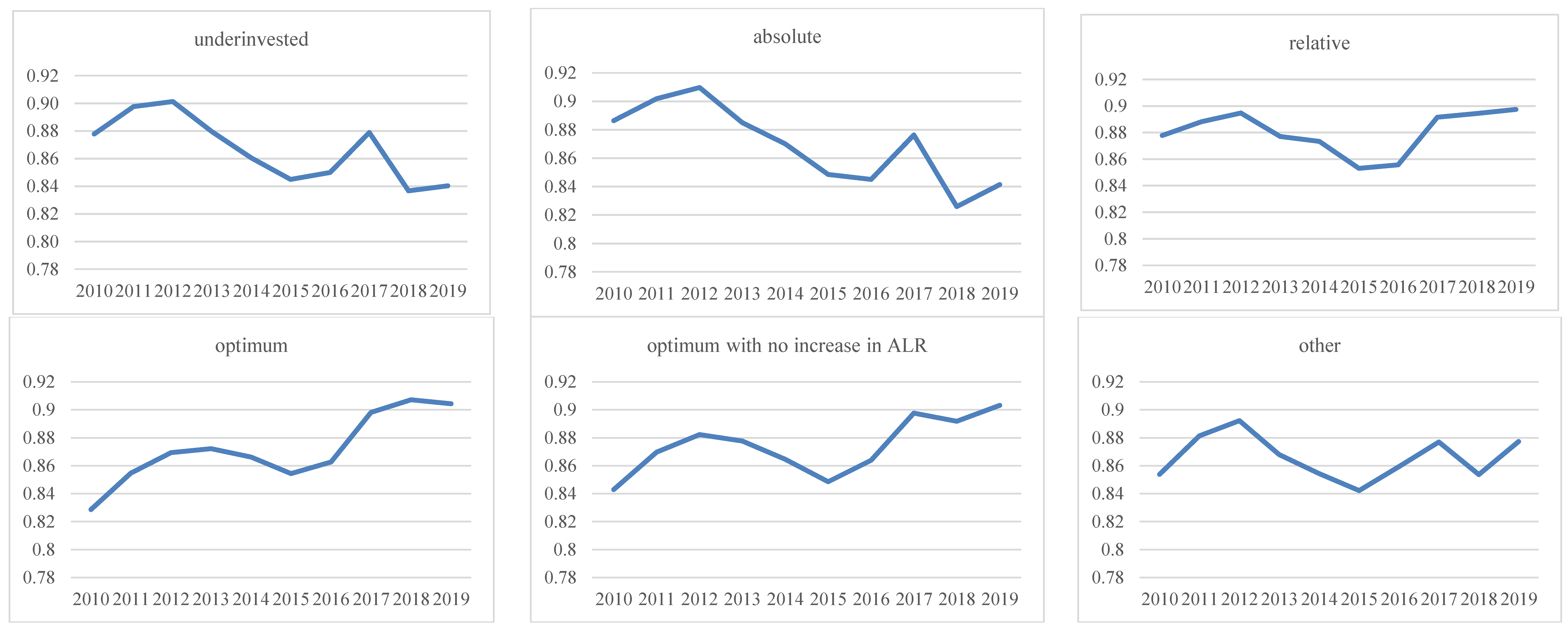
3. Results and Discussion
4. Conclusions
Author Contributions
Funding
Institutional Review Board Statement
Data Availability Statement
Conflicts of Interest
References
- Chloupkova, J. Polish Agriculture: Organisational Structure and Impacts of Transition; Unit of Economics Working Papers 24186; Royal Veterinary and Agricultural University, Food and Resource Economic Institute: Frederiksberg, Denmark, 2002. [Google Scholar] [CrossRef]
- Mrówczynska-Kamińska, A. Znaczenie rolnictwa w gospodarce narodowej w Polsce, analiza makroekonomiczna i regionalna. Zeszyty Naukowe Szkoły Głównej Gospodarstwa Wiejskiego w Warszawie. Problemy Rolnictwa Światowego 2008, 5, 96–108. [Google Scholar] [CrossRef]
- Szczukocka, A. Rozwój sektora rolnego w Polsce i krajach Unii Europejskiej [Development of the Agricultural Sector in Poland and European Union Countries]. Zeszyty Naukowe SGGW w Warszawie-Problemy Rolnictwa Światowego 2018, 18, 275–286. [Google Scholar] [CrossRef]
- Carvalho, F.P. Agriculture, pesticides, food security and food safety. Environ. Sci. Policy 2006, 9, 685–692. [Google Scholar] [CrossRef]
- FAO. Food and Agriculture: Key to Achieving the 2030 Agenda for Sustainable Development; Job No. I5499; Food and Agriculture Organization of the United Nations: Rome, Italy, 2016; p. 23. [Google Scholar]
- Guo, H.; Xia, Y.; Jin, J.; Pan, C. The impact of climate change on the efficiency of agricultural production in the world’s main agricultural regions. Environ. Impact Assess. Rev. 2022, 97, 106891. [Google Scholar] [CrossRef]
- Qi, Y.; Zhang, J.; Chen, X.; Li, Y.; Chang, Y.; Zhu, D. Effect of farmland cost on the scale efficiency of agricultural production based on farmland price deviation. Habitat Int. 2023, 132, 102745. [Google Scholar] [CrossRef]
- Wassie, S.B. Technical Efficiency of Major Crops in Ethiopia: Stochastic Frontier Model. Master’s Thesis, University of Oslo, Oslo, Norway, 2014. [Google Scholar]
- Żmija, D. Dylematy dotyczące aktywnej roli państwa w obszarze rolnictwa [Dilemmas in Active State Participation in Agriculture]. Zeszyty Naukowe Uniwersytetu Ekonomicznego w Krakowie 2011, 863, 53–68. [Google Scholar]
- Kanianska, R. Agriculture and its impact on land-use, environment, and ecosystem services. In Landscape Ecology—The Influences of Land Use and Anthropogenic Impacts of Landscape Creation; IntechOpen: London, UK, 2016; pp. 1–26. [Google Scholar] [CrossRef]
- FAO. The Future of Food and Agriculture. Trends and Challenges; Food and Agriculture Organization of the United Nations: Rome, Italy, 2017. [Google Scholar]
- Gebbers, R.; Adamchuk, V.I. Precision agriculture and food security. Science 2010, 327, 828–831. [Google Scholar] [CrossRef]
- Michalczyk, J. The Impact of the Common Agricultural Policy on the Development of Polish Agri-food Sector. Zeszyty Naukowe Uniwersytetu Szczecińskiego. Finanse, Rynki Finansowe, Ubezpieczenia 2011, 43, 107–118. [Google Scholar] [CrossRef]
- Czubak, W.; Sadowski, A.; Wigier, M.; Mrówczyńska-Kamińska, A. Inwestycje w Rolnictwie Polskim po Integracji z Unią Europejską [Investments in Polish Agriculture after the Integration into the European Union]; Wyd. Uniwersytetu Przyrodniczego w Poznaniu: Poznań, Poland, 2014. [Google Scholar]
- Kiryluk-Dryjska, E.; Beba, P.; Poczta, W. Local determinants of the Common Agricultural Policy rural development funds’ distribution in Poland and their spatial implications. J. Rural Stud. 2020, 74, 201–209. [Google Scholar] [CrossRef]
- Ricker-Gilbert, J.; Jayne, T.S. What Are the Enduring Effects of Fertilizer Subsidy Programs on Recipient Farm Households? Evidence from Malawi; Staff Paper Series 109593; Michigan State University, Department of Agricultural, Food, and Resource Economics: East Lansing, MI, USA, 2011. [Google Scholar] [CrossRef]
- Wang, S.W.; Manjur, B.; Kim, J.G.; Lee, W.K. Assessing socio-economic impacts of agricultural subsidies: A case study from Bhutan. Sustainability 2019, 11, 3266. [Google Scholar] [CrossRef]
- Smędzik-Ambroży, K.; Guth, M.; Stępień, S.; Brelik, A. The influence of the European Union’s common agricultural policy on the socio-economic sustainability of farms (the case of Poland). Sustainability 2019, 11, 7173. [Google Scholar] [CrossRef]
- Kiryluk-Dryjska, E.; Baer-Nawrocka, A. Reforms of the Common Agricultural Policy of the EU: Expected results and their social acceptance. J. Policy Model. 2019, 41, 607–622. [Google Scholar] [CrossRef]
- Gabel, M.; Palmer, H.D. Understanding variation in public support for European integration. Eur. J. Political Res. 1995, 27, 3–19. [Google Scholar] [CrossRef]
- Zalewski, K.; Bórawski, P.; Żuchowski, I.; Parzonko, A.; Holden, L.; Rokicki, T. The Efficiency of Public Financial Support Investments into Dairy Farms in Poland by the European Union. Agriculture 2022, 12, 186. [Google Scholar] [CrossRef]
- Winters, L.A. The economic consequences of agricultural support: A survey. OECD Econ. Stud. 1987, 9, 7–54. [Google Scholar] [CrossRef]
- Schulte, H.D.; Musshoff, O.; Meuwissen, M.P.M. Considering milk price volatility for investment decisions on the farm level after European milk quota abolition. J. Dairy Sci. 2018, 101, 7531–7539. [Google Scholar] [CrossRef]
- Alcon, F.; Tapsuwan, S.; Brouwer, R.; Yunes, M.; Mounzer, O.; de-Miguel, M.D. Modelling farmer choices for water security measures in the Litani river basin in Lebanon. Sci. Total Environ. 2019, 647, 37–46. [Google Scholar] [CrossRef]
- Judzińska, A.; Łopaciuk, W. Wpływ Wspólnej Polityki Rolnej na Rolnictwo [The Impact of the Common Agricultural Policy on Agriculture]; Instytut Ekonomiki Rolnictwa i Gospodarki Żywnościowej-Państwowy Instytut Badawczy: Warsaw, Poland, 2011. [Google Scholar]
- Bórawski, P.; Guth, M.; Bełdycka-Bórawska, A.; Jankowski, K.J.; Parzonko, A.; Dunn, J.W. Investments in Polish agriculture: How production factors shape conditions for environmental protection? Sustainability 2020, 12, 8160. [Google Scholar] [CrossRef]
- Kata, R. Kredyty bankowe w strukturze zewnętrznych źródeł finansowania rolnictwa w Polsce [Bank credits in the structure of external sources of financing agriculture in Poland]. Problemy Rolnictwa Światowego 2009, 8, 85–97. [Google Scholar] [CrossRef]
- Zidkova, D.; Rezbova, H.; Rosochatecka, E. Analysis of development of investments in the agricultural sector of the Czech Republic. Agris-Line Pap. Econ. Inform. 2011, 3, 33–43. [Google Scholar] [CrossRef]
- Barret, S. Climate treaties and “breakthrough” technologies. Am. Econ. Rev. 2006, 96, 22–25. [Google Scholar] [CrossRef]
- Ogundari, K. The Paradigm of Agricultural Efficiency and its Implication on Food Security in Africa: What Does Meta-analysis Reveal? World Dev. 2014, 64, 690–702. [Google Scholar] [CrossRef]
- Kebede, D.; Emana, B.; Tesfay, G. Impact of land acquisition for large-scale agricultural investments on food security status of displaced households: The case of Ethiopia. Land Use Policy 2023, 126, 106507. [Google Scholar] [CrossRef]
- Estrada-Carmona, N.; Raneri, J.E.; Alvarez, S.; Timler, C.; Chatterjee, S.A.; Ditzler, L.; Kennedy, G.; Remans, R.; Brouwer, I.; Borgonjen-van den Berg, K.; et al. A model-based exploration of farm-household livelihood and nutrition indicators to guide nutrition-sensitive agriculture interventions. Food Secur. 2019, 12, 59–81. [Google Scholar] [CrossRef]
- Brooks, J. Policy coherence and food security: The effects of OECD countries agricultural policies. Food Policy 2014, 44, 88–94. [Google Scholar] [CrossRef]
- Baer-Nawrocka, A.; Sadowski, A. Food security and food self-sufficiency around the world: A typology of countries. PLoS ONE 2019, 14, e0213448. [Google Scholar] [CrossRef]
- Cassman, K.G.; Harwood, R.R. The nature of agricultural systems: Food security and environmental balance. Food Policy 1995, 20, 439–454. [Google Scholar] [CrossRef]
- Brevik, E.C.; Calzolari, C.; Miller, B.A.; Pereira, P.; Kabala, C.; Baumgarten, A.; Jordán, A. Soil mapping, classification, and pedologic modeling: History and future directions. Geoderma 2016, 264, 256–274. [Google Scholar] [CrossRef]
- Viana, C.M.; Freire, D.; Abrantes, P.; Rocha, J.; Pereira, P. Agricultural land systems importance for supporting food security and sustainable development goals: A systematic review. Sci. Total Environ. 2022, 806, 150718. [Google Scholar] [CrossRef]
- Peña-Arancibia, J.L.; Malerba, M.E.; Wright, N.; Robertson, D.E. Characterising the regional growth of on-farm storages and their implications for water resources under a changing climate. J. Hydrol. 2023, 625, 130097. [Google Scholar] [CrossRef]
- Pimentel, J.; Balázs, L.; Friedler, F. Optimization of vertical farms energy efficiency via multiperiodic graph-theoretical approach. J. Clean. Prod. 2023, 416, 137938. [Google Scholar] [CrossRef]
- Pawłowski, K.P.; Czubak, W.; Zmyślona, J. Regional Diversity of Technical Efficiency in Agriculture as a Results of an Overinvestment: A Case Study from Poland. Energies 2021, 14, 3357. [Google Scholar] [CrossRef]
- Zmyślona, J.; Sadowski, A.; Genstwa, N. Plant Protection and Fertilizer Use Efficiency in Farms in a Context of Overinvestment: A Case Study from Poland. Agriculture 2023, 13, 1567. [Google Scholar] [CrossRef]
- Chen, X.; Sun, Y.; Xu, X. Free cash flow, over-investment and corporate governance in China. Pac.-Basin Financ. J. 2016, 37, 81–103. [Google Scholar] [CrossRef]
- Mukherji, A.; Nagarajan, N.J. Moral hazard and contractibility in investment decisions. J. Econ. Behav. Organ. 1995, 26, 413–430. [Google Scholar] [CrossRef]
- Lerman, Z.; Csaki, C.; Feder, G. Land Policies and Evolving Farm Structures in Transition Countries; World Bank: Washington, DC, USA, 2002; p. 49. [Google Scholar] [CrossRef]
- Yu, X.; Yao, Y.; Zheng, H.; Zhang, L. The role of political connection on overinvestment of Chinese energy firms. Energy Econ. 2020, 85, 104516. [Google Scholar] [CrossRef]
- Zhang, D.; Cao, H.; Zou, P. Exuberance in China’s renewable energy investment: Rationality, capital structure and implications with firm level evidence. Energy Policy 2016, 95, 468–478. [Google Scholar] [CrossRef]
- Stiglitz, J.E.; Weiss, A. Credit Rationing in Markets with Imperfect Information. Am. Econ. Rev. 1981, 71, 393–410. [Google Scholar]
- Haramillo, F.; Schiantarelli, F.; Weiss, A. Capital market imperfections before and after financial liberalization: An Euler equation approach to panel data for Ecuadorian firms. J. Dev. Econ. 1996, 51, 367–386. [Google Scholar] [CrossRef]
- Zmyślona, J.; Sadowski, A. Overinvestment in polish agriculture. In Proceedings of the 2019 International Scientific Conference ‘Economic Sciences for Agribusiness and Rural Economy, Warsaw, Poland, 5–7 June 2019; Warsaw University of Life Sciences Press: Warsaw, Poland, 2019; Volume 3, pp. 152–154. [Google Scholar]
- D’Mello, R.; Miranda, M. Long-term and overinvestment agency problem. J. Bak. Financ. 2010, 34, 324–335. [Google Scholar] [CrossRef]
- Lin, Y.C. Do Voluntary Clawback Adoptions Curb Overinvestment. Corp. Gov. Int. Rev. 2017, 25, 255–270. [Google Scholar] [CrossRef]
- Wang, S.; Wan, J.; Li, D.; Zhang, C. Implementing Smart Factory of Industrie 4.0: An Outlook. Int. J. Distrib. Sens. Netw. 2016, 12, 3159805. [Google Scholar] [CrossRef]
- Wei, X.; Wang, C.; Guo, Y. Does quasi-mandatory dividend rule restrain overinvestment? Int. Rev. Econ. Financ. 2019, 63, 4–23. [Google Scholar] [CrossRef]
- Pellicani, A.D.; Kalatzis, A.E.G. Ownership structure, overinvestent and underinvestment: Evidence from Brazil. Res. Int. Bus. Finans. 2018, 48, 475–482. [Google Scholar] [CrossRef]
- Schnabl, G. China’s Overinvestment and International Trade Conflicts. China World Econ. 2019, 27, 37–62. [Google Scholar] [CrossRef]
- Nghia, N.T.; Khang, T.L.; Thanh, N.C. The Moderation Effect of Debt and Dividend on the Overinvestment-Performance Relationship. In Beyond Traditional Probabilistic Methods in Economics; Studies in Computational Intelligence, ECONVN 2019; Springer: Berlin/Heidelberg, Germany, 2019; Volume 809, pp. 1109–1120. [Google Scholar] [CrossRef]
- Poczta, W.; Średzińska, J. Wyniki produkcyjno-ekonomiczne i finansowe indywidualnych gospodarstw rolnych według ich wielkości ekonomicznej (na przykładzie regionu FADN, Wielkopolska i Śląsk) [Production-economic and financial performance of individual farms according to their economic size (on the example of the FADN region, Wielkopolska and Silesia)]. Zeszyty Naukowe Szkoły Głównej Gospodarstwa Wiejskiego w Warszawie Problemy Rolnictwa Światowego 2007, 2, 433–443. [Google Scholar] [CrossRef]
- Feng, Y.; Zhang, Y.; Li, S.; Wang, C.; Yin, X.; Chu, Q.; Chen, F. Sustainable options for reducing carbon inputs and improving the eco-efficiency of smallholder wheat-maize cropping systems in the Huanghuaihai Farming Region of China. J. Clean. Prod. 2020, 244, 118887. [Google Scholar] [CrossRef]
- Ding, S.; Knight, J.; Zhang, X. Does China overinvest? Evidence from a panel of Chinese firms. Eur. J. Financ. 2019, 25, 489–507. [Google Scholar] [CrossRef]
- Guan, Z.; Kumbhakar, S.C.; Myers, R.J.; Lansink, A.O. Measuring excess capital capacity in agricultural production. Am. J. Agric. Econ. 2009, 91, 765–776. [Google Scholar] [CrossRef]
- Samuelson, P.A.; Nordhaus, W.D. Ekonomia [Economics]; Dom Wydawniczy REBIS: Poznań, Poland, 2012. [Google Scholar]
- Garrido, A.; Brümmer, B.; M’Barek, R.; Meuwissen, M.; Morales-Opazo, C. Agricultural Markets Instability: Revisiting the Recent Food Crises; Routledge: London, UK, 2016. [Google Scholar]
- Ciaian, P.; Kancsy, D.A.; Michalek, J. Investment Crowding-Out: Firm-Level Evidence from Germany; LICOS Discussion Paper Series; Disussion Paper 370/2015; LICOS Centre for Institutions and Economic Performance: Leuven, Belgium, 2015. [Google Scholar]
- Anania, G.; Blom, J.C.; Buckwell, A.; Colson, F.; Azcarate, T.G.; Mathurin, J.; Rabinowicz, E.; Saraceno, E.; Sumpsi, J.; von Urff, W.; et al. Policy Vision for Sustainable Rural Economies in an Enlarged Europe; Studies in Spatial Development, No. 4; Verlag der ARL—Akademie für Raumforschung und Landesplanung: Hannover, Germany, 2003. [Google Scholar]
- Chivu, L.; Andrei, J.V.; Zahariav, M.; Gogonea, R.M. A regional agricultural efficiency convergence assessment in Romania–Appraising differences and understanding potentials. Land Use Policy 2020, 99, 104838. [Google Scholar] [CrossRef]
- Špička, J.; Smutka, L. The technical efficiency of specialised milk farms: A regional view. Sci. World J. 2014, 2014, 985149. [Google Scholar] [CrossRef] [PubMed]
- Ghoshal, P.; Goswami, B. Cobb-douglas production function for measuring efficiency in indian agriculture: A region-wise analysis. Econ. Aff. 2017, 62, 573–579. [Google Scholar] [CrossRef]
- Khatri-Chhetri, A.; Sapkota, T.B.; Maharjan, S.; Konath, N.C.; Shirsath, P. Agricultural emissions reduction potential by improving technical efficiency in crop production. Agric. Syst. 2023, 207, 103620. [Google Scholar] [CrossRef]
- Islam, S.; Mitra, S.; Khan, M.A. Technical and cost efficiency of pond fish farms: Do young educated farmers bring changes? J. Agric. Food Res. 2023, 12, 100581. [Google Scholar] [CrossRef]
- Vogel, E.; Dalheimer, B.; Beber, C.L.; de Mori, C.; Palhares, J.C.P.; Novo, A.L.M. Environmental efficiency and methane abatement costs of dairy farms from Minas Gerais, Brazil. Food Policy 2023, 119, 102520. [Google Scholar] [CrossRef]
- Tamirat, N.; Tadele, S. Determinants of technical efficiency of coffee production in Jimma Zone, Southwest Ethiopia. Heliyon 2023, 9, e15030. [Google Scholar] [CrossRef]
- Zozimo, T.M.; Kawube, G.; Kalule, S.W. The role of development interventions in enhancing technical efficiency of sunflower producers. J. Agric. Food Res. 2023, 14, 100707. [Google Scholar] [CrossRef]
- Ngango, J.; Hong, S. Assessing production efficiency by farm size in Rwanda: A zero-inefficiency stochastic frontier approach. Sci. Afr. 2022, 16, e01143. [Google Scholar] [CrossRef]
- Li, K.; Zou, D.; Li, H. Environmental regulation and green technical efficiency: A process-level data envelopment analysis from Chinese iron and steel enterprises. Energy 2023, 277, 127662. [Google Scholar] [CrossRef]
- Molinos-Senante, M.; Maziotis, A.; Sala-Garrido, R.; Mocholi-Arce, M. An investigation of productivity, profitability, and regulation in the Chilean water industry using stochastic frontier analysis. Decis. Anal. J. 2022, 4, 100117. [Google Scholar] [CrossRef]
- Fousekis, P.; Spathis, P.; Tsimboukas, K. Assessing the efficiency of sheep farming in mountainous areas of Greece. A non parametric approach. Agric. Econ. Rev. 2001, 2, 5–15. [Google Scholar] [CrossRef]
- Floriańczyk, Z.; Osuch, D.; Płonka, R. Wyniki Standardowe 2017 Uzyskane Przez Gospodarstwa Rolne Uczestniczące w Polskim FADN [Standard Results 2017 Obtained by Farms Participating in the Polish FADN]; Część I. Wyniki Standardowe Polski FADN; IERiGŻ-PIB, Zakład Rachunkowości Rolnej: Warsaw, Poland, 2018. [Google Scholar]
- Gołaś, Z. Systemy wskaźników dochodowości pracy w rolnictwie–propozycja metodyczna [Systems of labor profitability indicators in agriculture—Methodological proposal]. Zeszyty Naukowe Szkoły Głównej Gospodarstwa Wiejskiego Ekonomika i Organizacja Gospodarki Żywnościowej 2015, 109, 17–26. [Google Scholar] [CrossRef]
- Aigner, D.; Lovell, C.K.; Schmidt, P. Formulation and estimation of stochastic frontier production function models. J. Econom. 1977, 6, 21–37. [Google Scholar] [CrossRef]
- Meeusen, W.; van Den Broeck, J. Efficiency estimation from Cobb-Douglas production functions with composed error. Int. Econ. Rev. 1977, 18, 435–444. [Google Scholar] [CrossRef]
- Ruggiero, J.; Vitaliano, D.F. Assessing the efficiency of public schools using data envelopment analysis and frontier regression. Contemp. Econ. Policy 1999, 17, 321–331. [Google Scholar] [CrossRef]
- Pitt, M.M.; Lee, L.F. The measurement and sources of technical inefficiency in the Indonesian weaving industry. J. Dev. Econ. 1981, 9, 43–64. [Google Scholar] [CrossRef]
- Battese, G.E.; Coelli, T.J. Prediction of firm-level technical efficiencies with a generalized frontier production function and panel data. J. Econom. 1988, 38, 387–399. [Google Scholar] [CrossRef]
- Schmidt, P.; Sickles, R.C. Production frontiers and panel data. J. Bus. Econ. Stat. 1984, 2, 367–374. [Google Scholar] [CrossRef]
- Cornwell, C.; Schmidt, P.; Sickles, R.C. Production frontiers with cross-sectional and time-series variation in efficiency levels. J. Econom. 1990, 46, 185–200. [Google Scholar] [CrossRef]
- Kumbhakar, S.C.; Sun, K. Derivation of marginal effects of determinants of technical inefficiency. Econ. Lett. 2013, 120, 249–253. [Google Scholar] [CrossRef]
- Coelli, T.J.; Rao, D.S.P.; O’Donnell, C.J.; Battese, G.E. An Introduction to Efficiency and Productivity Analysis; Springer Science Business Media: New York, NY, USA, 2005. [Google Scholar] [CrossRef]
- Greene, W.H. Frontier Production Functions; Working Papers 93-20; Stern School of Business, New York University: New York, NY, USA, 1993. [Google Scholar] [CrossRef]
- Bezat-Jarzębowska, A.; Rembisz, W. Wprowadzenie do Analizy Inwestycji, Produktywności, Efektywności i Zmian Technicznych w Rolnictwie [Introduction to the Analysis of Investment, Productivity, Efficiency and Technical Change in Agriculture]; Instytut Ekonomiki Rolnictwa i Gospodarki Żywnościowej-Państwowy Instytut Badawczy: Warsaw, Poland, 2015. [Google Scholar]
- Umar, H.S.; Girei, A.A.; Yakubu, D. Comparison of Cobb-Douglas and Translog frontier models in the analysis of technical efficiency in dry-season tomato production. Agrosearch 2017, 17, 67–77. [Google Scholar] [CrossRef]
- Coelli, T.J.; Battese, G.E. Identification of factors which influence the technical inefficiency of Indian farmers. Aust. J. Agric. Econ. 1996, 40, 103–128. [Google Scholar] [CrossRef]
- Coelli, T.J. Recent developments in frontier modelling and efficiency measurement. Aust. J. Agric. Econ. 1995, 39, 219–245. [Google Scholar] [CrossRef]
- Zepeda, L. Agricultural Investment, Production Capacity and Productivity; FAO Economic and Social Development Paper; Food and Agriculture Organization of the United Nations: Rome, Italy, 2001; pp. 3–20. [Google Scholar]
- Gaviglio, A.; Filippini, R.; Madau, F.A.; Marescotti, M.E.; Demartini, E. Technical efficiency and productivity of farms: A periurban case study analysis. Agric. Food Econ. 2021, 9, 11. [Google Scholar] [CrossRef]
- Pawłowska, A.; Rembisz, W. Źródła wzrostu wydajności czynnika pracy w polskim sektorze rolnym. Stud. Ekon. 2020, 395, 80–91. [Google Scholar]
- Góral, J.; Rembisz, W. Wydajność pracy i czynniki ją kształtujące w polskim rolnictwie w latach 2000–2015. Wieś i Rolnictwo 2017, 4, 17–37. [Google Scholar] [CrossRef]

| Variable (Unit) | Overinvestment Group | Mean | Std. Dev. | Min. | Max. | ||||
|---|---|---|---|---|---|---|---|---|---|
| 2010 | 2019 | 2010 | 2019 | 2010 | 2019 | 2010 | 2019 | ||
| Q: SE131 (PLN thousand) | underinvested | 185.37 | 199.82 | 312.12 | 368.60 | −12.25 | −12.41 | 5114.00 | 5766.09 |
| other | 111.91 | 117.92 | 161.62 | 197.40 | 2.67 | 5.84 | 1589.01 | 1877.48 | |
| optimum investment, no increase in ALR | 217.60 | 351.31 | 352.27 | 578.71 | 12.12 | 6.52 | 3720.03 | 5478.26 | |
| optimum investment, increase in ALR and LP | 325.33 | 620.29 | 998.22 | 1580.48 | 11.75 | 11.53 | 18,800.00 | 30,200.00 | |
| absolute | 315.78 | 360.05 | 759.91 | 594.86 | 21.74 | 5.92 | 14,700.00 | 7688.76 | |
| relative | 435.56 | 616.22 | 1374.99 | 1224.53 | 9.45 | 11.51 | 14,500.00 | 10,500.00 | |
| L: SE010 (ha) | underinvested | 1.80 | 1.89 | 0.97 | 1.11 | 0.25 | 0.20 | 12.89 | 17.96 |
| other | 1.80 | 1.379 | 1.57 | 0.72 | 0.46 | 0.20 | 27.27 | 6.50 | |
| optimum investment, no increase in ALR | 2.07 | 2.29 | 1.81 | 2.43 | 0.33 | 0.44 | 30.05 | 46.89 | |
| optimum investment, increase in ALR and LP | 2.64 | 2.48 | 5.27 | 4.69 | 0.62 | 0.28 | 111.35 | 95.00 | |
| absolute | 2.34 | 1.97 | 3.23 | 1.86 | 0.66 | 0.17 | 61.99 | 26.74 | |
| relative | 2.86 | 2.42 | 5.29 | 3.45 | 0.73 | 0.22 | 66.13 | 40.41 | |
| Z: SE025 (ha) | underinvested | 34.05 | 34.42 | 57.94 | 55.23 | 0.00 | 0.07 | 906.00 | 963.00 |
| other | 20.23 | 17.76 | 20.68 | 17.71 | 0.08 | 0.00 | 163.89 | 158.98 | |
| optimum investment, no increase in ALR | 31.90 | 38.04 | 45.11 | 54.79 | 0.00 | 0.00 | 743.00 | 715.00 | |
| optimum investment, increase in ALR and LP | 49.43 | 57.84 | 162.36 | 147.18 | 0.00 | 0.00 | 2654.00 | 2424.61 | |
| absolute | 56.88 | 58.35 | 128.97 | 84.06 | 0.00 | 0.00 | 2126.00 | 1288.69 | |
| relative | 73.96 | 77.40 | 283.43 | 242.34 | 0.00 | 0.00 | 3487.70 | 3141.24 | |
| K: SE441-SE446 (EUR thousand) | underinvested | 147.09 | 179.28 | 272.31 | 356.27 | 10.41 | 6.61 | 4860.00 | 6099.40 |
| other | 92.44 | 89.67 | 131.39 | 157.03 | 11.45 | 10.48 | 1287.90 | 1849.45 | |
| optimum investment, no increase in ALR | 175.02 | 249.65 | 285.86 | 442.45 | 13.67 | 15.34 | 3078.73 | 5213.12 | |
| optimum investment, increase in ALR and LP | 276.63 | 471.58 | 1088.77 | 1634.06 | 13.23 | 12.79 | 20,900.00 | 32,600.00 | |
| Specification | Coeff. | Std. err. | P > |z| |
|---|---|---|---|
| Frontier | |||
| lnK | 0.7245 | 0.0057 | 0.000 |
| lnL | 0.1047 | 0.0063 | 0.000 |
| lnZ | 0.1494 | 0.0076 | 0.000 |
| Usigma | |||
| _cons | −3.8432 | 0.0265 | 0.000 |
| Vsigma | |||
| _cons | −3.9453 | 0.0181 | 0.000 |
| sigma_u | 0.1464 | 0.0019 | 0.000 |
| sigma_v | 0.1391 | 0.0013 | 0.000 |
| lambda | 1.0524 | 0.0029 | 0.000 |
| Frontier | Usigma | Vsigma | ||||||||||
|---|---|---|---|---|---|---|---|---|---|---|---|---|
| Coeff. | Std. err. | P > |z| | Coeff. | Std. err. | P > |z| | Coeff. | Std. err. | P > |z| | ||||
| underinvested | lnK | 0.7240 | 0.0117 | 0.000 | _cons | −3.5697 | 0.0415 | 0.000 | _cons | −4.0027 | 0.0336 | 0.000 |
| lnL | 0.0719 | 0.0135 | 0.000 | - | - | - | - | sigma_u | 0.1678 | 0.0035 | 0.000 | |
| lnZ | 0.1824 | 0.0174 | 0.000 | - | - | - | - | sigma_v | 0.1351 | 0.0023 | 0.000 | |
| - | - | - | - | - | - | - | - | lambda | 1.2417 | 0.0052 | 0.000 | |
| other | lnK | 0.7290 | 0.0197 | 0.000 | _cons | −3.6225 | 0.0772 | 0.000 | _cons | −3.9167 | 0.0587 | 0.000 |
| lnL | 0.0865 | 0.0170 | 0.000 | - | - | - | - | sigma_u | 0.1634 | 0.0063 | 0.000 | |
| lnZ | 0.0407 | 0.0211 | 0.053 | - | - | - | - | sigma_v | 0.1411 | 0.0041 | 0.000 | |
| - | - | - | - | - | - | - | - | lambda | 1.1585 | 0.0095 | 0.000 | |
| optimum investment, no increase in ALR | lnK | 0.7326 | 0.0144 | 0.000 | _cons | −4.1244 | 0.0719 | 0.000 | _cons | −3.9911 | 0.0432 | 0.000 |
| lnL | 0.1547 | 0.0164 | 0.000 | - | - | - | - | sigma_u | 0.1272 | 0.0046 | 0.000 | |
| lnZ | 0.1542 | 0.0167 | 0.000 | - | - | - | - | sigma_v | 0.1359 | 0.0029 | 0.000 | |
| - | - | - | - | - | - | - | - | lambda | 0.9355 | 0.0070 | 0.000 | |
| optimum investment, increase in ALR and LP | lnK | 0.8937 | 0.0125 | 0.000 | _cons | −4.4346 | 0.0941 | 0.000 | _cons | −3.7436 | 0.0396 | 0.000 |
| lnL | 0.0168 | 0.0157 | 0.000 | - | - | - | - | sigma_u | 0.1089 | 0.0051 | 0.000 | |
| lnZ | 0.1267 | 0.0159 | 0.000 | - | - | - | - | sigma_v | 0.1538 | 0.0030 | 0.000 | |
| - | - | - | - | - | - | - | - | lambda | 0.7078 | 0.0076 | 0.000 | |
| absolute | lnK | 0.5571 | 0.0124 | 0.000 | _cons | −3.7205 | 0.0559 | 0.000 | _cons | −4.0650 | 0.0441 | 0.000 |
| lnL | 0.2076 | 0.0131 | 0.000 | - | - | - | - | sigma_u | 0.1556 | 0.0043 | 0.000 | |
| lnZ | 0.1835 | 0.0171 | 0.000 | - | - | - | - | sigma_v | 0.1310 | 0.0029 | 0.000 | |
| - | - | - | - | - | - | - | - | lambda | 1.1880 | 0.0066 | 0.000 | |
| relative | lnK | 0.6814 | 0.0166 | 0.000 | _cons | −4.5922 | 0.1394 | 0.000 | _cons | −4.0922 | 0.0663 | 0.000 |
| lnL | 0.0585 | 0.0200 | 0.003 | - | - | - | - | sigma_u | 0.1006 | 0.0070 | 0.000 | |
| lnZ | 0.1988 | 0.0245 | 0.000 | - | - | - | - | sigma_v | 0.1292 | 0.0043 | 0.000 | |
| - | - | - | - | - | - | - | - | lambda | 0.7788 | 0.0105 | 0.000 | |
| Specification | Underinvested | Other | Optimum Investment, No Increase in ALR | Optimum Investment, Increase in ALR and LP | Absolute | Relative |
|---|---|---|---|---|---|---|
| sigma_u | 0.1678 | 0.1634 | 0.1272 | 0.1089 | 0.1556 | 0.1006 |
| sigma_v | 0.1351 | 0.1411 | 0.1359 | 0.1538 | 0.1310 | 0.1292 |
| %u | 60.66% | 57.30% | 46.67% | 33.38% | 58.53% | 37.76% |
| %v | 39.34% | 42.70% | 53.33% | 66.62% | 41.47% | 62.24% |
Disclaimer/Publisher’s Note: The statements, opinions and data contained in all publications are solely those of the individual author(s) and contributor(s) and not of MDPI and/or the editor(s). MDPI and/or the editor(s) disclaim responsibility for any injury to people or property resulting from any ideas, methods, instructions or products referred to in the content. |
© 2024 by the authors. Licensee MDPI, Basel, Switzerland. This article is an open access article distributed under the terms and conditions of the Creative Commons Attribution (CC BY) license (https://creativecommons.org/licenses/by/4.0/).
Share and Cite
Zmyślona, J.; Sadowski, A.; Pawłowski, K.P. How Can Overinvestment in Farms Affect Their Technical Efficiency? A Case Study from Poland. Agriculture 2024, 14, 1799. https://doi.org/10.3390/agriculture14101799
Zmyślona J, Sadowski A, Pawłowski KP. How Can Overinvestment in Farms Affect Their Technical Efficiency? A Case Study from Poland. Agriculture. 2024; 14(10):1799. https://doi.org/10.3390/agriculture14101799
Chicago/Turabian StyleZmyślona, Jagoda, Arkadiusz Sadowski, and Krzysztof Piotr Pawłowski. 2024. "How Can Overinvestment in Farms Affect Their Technical Efficiency? A Case Study from Poland" Agriculture 14, no. 10: 1799. https://doi.org/10.3390/agriculture14101799
APA StyleZmyślona, J., Sadowski, A., & Pawłowski, K. P. (2024). How Can Overinvestment in Farms Affect Their Technical Efficiency? A Case Study from Poland. Agriculture, 14(10), 1799. https://doi.org/10.3390/agriculture14101799