Investigation on Zoning Management of Saline Soil in Cotton Fields in Alar Reclamation Area, Xinjiang

Abstract

Aiming at assessing the problems of the high land salinity, high spatial variability of soil nutrients, sloppy management, and low efficiency in the Xinjiang region, research on the precise delineation method of field management zones is being conducted to facilitate differentiated fertilizer management for farmers and increase the level of saline soil improvement. Taking the plots in the experimental area as the research object, traditional statistics, principal component analysis, and fuzzy c-mean classification were applied to divide the management zoning in the study area, and the suitability and effectiveness of the management zoning were evaluated. The study area was at a mild salinization level; the soil organic matter and total nitrogen content were at a low level; total phosphorus was at a medium level; and total potassium and pH reached a high level. pH had a coefficient of variation <0.1, which was weak, and the other soil attributes were of medium variability intensity. The spatial distribution of the soil attributes was highly variable. The results of the principal component analysis showed that the six soil attributes grouped into statistical factors could be divided into three principal components. The results of the fuzzy c-means classification showed that the study area could be divided into four management zones, and there were significant differences in the soil salinity, organic matter, soil nutrients, and other attributes in the different management zones. The different soil attributes could be utilized to determine the management zoning of farmland in the study area with the help of fuzzy c-mean classification.

1. Introduction

Soil salinization is a dynamic and changing ecological process that has significant impacts on soil, hydrology, climate, agriculture, and economy [1]. In addition, the conversion of natural high-quality soils to salinized soils is accelerated because of temperature increase, precipitation fluctuation, and anthropogenic factors caused by climate change [1,2,3,4]. At the same time, the improper cultivation of a large number of crops and the irrational utilization of water resources in the Tarim Basin have led to a series of ecological disasters such as vegetation degradation, dust storms, land desertification, land salinization, and so on. In recent decades, soil erosion has intensified since the rapid development of land use in Xinjiang, which leads to an obvious spatial heterogeneity in the degree of soil salinization [5]. The spatial distribution of soil salinity is influenced by various environmental factors, such as topography, vegetation abundance, climatic conditions and land use, and changes with the geographic environment. Soil salinity is an important factor limiting plant growth and regional stability because it not only affects soil properties and leads to decreased soil fertility but also influences plant species diversity and causes crop yield reduction [6,7]. In accordance with the field and geographical point of view, it is necessary to monitor the salinity in the soil profile of arable land, in a timely and effective manner, to have a clear understanding of its spatial distribution trend, to divide salinized soil into different areas, and then to use the salinity level in which the field is located to guide the precise irrigation of arable land and the rational layout of crops [8].

Similar to the topography and arable soil conditions in management zonation, the crop productivity, nutrient use efficiency, and environmental effect sub-regions are almost similar [9]. According to the specific situation of each management partition in a studied field, a differentiated soil management approach is adopted to regulate the application of input substances accordingly [10]. This approach not only improves the efficiency of arable land use, but also enhances the output and quality of agricultural products, conserves resources, and thus yields desired economic benefits, which in turn protects agricultural resources and environmental quality. Based on the spatial and temporal variability and spatial autocorrelation of soil nutrient elements, the implementation of variable factor regulation on arable land is a frontier topic in the field of fine agriculture. The published studies mainly focus on the current status of land use, land resource characteristics, and the land use demand of determining the scope of land management zoning, objectives, and management measures [11]. At the same time, it is also explored in [11] how to use modern technical means such as GIS and remote sensing technology to improve the accuracy and effectiveness of its zoning. On the other hand, some existing results focus more on zoning ecological issues and sustainable development issues [12]. Some countries and regions have established mature soil management zoning systems and management mechanisms, and have achieved remarkable results [13]. Metwally M S et al.’s MZs were delineated by performing principal component analysis (PCA) and fuzzy K-means clustering. Four PCs with eigen values of more than 1 dominated 84.44% of the total variance, so they were retained for the clustering analysis. Three MZs were delineated based on the two criteria, modified partition entropy (MPE) and fuzzy performance index (FPI). The studied soil properties differed significantly among the MZs. Thus, the methodology used for MZ delineation could be used effectively for soil site-specific nutrient management for avoiding soil degradation concurrently with maximizing crop production in the study area [14]. Shukla M K et al. used principle component (PC) analysis and the fuzzy k-means technique for the precision management of large diversified farms. The PCA analysis showed that the first three PCs explained 73% of the variation with PC1, consisting of factors related to the soil’s physical condition; PC2, containing factors related to chemical properties; and PC3, including factors related to macro- and micro-porosities. Minimizing the fuzziness performance index (FPI) and modified partition entropy (MPE) delineated four management classes [15]. Jaynes et al. used cluster analysis to apply crop yield information to the management and partitioning of areas [16]. Techen A K et al. have distinguished four categories of soil management practices: spatial arrangements of cropping systems, crops and rotations, mechanical pressures, and inputs into the soil. The key research needs identified for each include nutrient efficiency in agroforestry versus conventional cropping systems, soil-rhizosphere microbiome elucidation to understand the interacting roles of crops and rotations, the effects of soil compaction on soil–plant–atmosphere interactions, and the ecotoxicity of plastics, pharmaceuticals, and other pollutants that are introduced into the soil. We establish an interdisciplinary, systemic approach to soil science and include cross-cutting research activities related to process modeling, data management, stakeholder interaction, sustainability assessment, and governance. The identification of soil research challenges from the perspective of agricultural management facilitates cooperation between different scientific disciplines in the field of sustainable agricultural production [17]. Gavioli A et al. evaluated the following algorithms: Average Linkage, Bagged Clustering, Centroid Linkage, Clara, Complete Linkage, Diana, Fanny, FCM, Fuzzy C-shells, Hard Competitive Learning, Hybrid Hierarchical Clustering, K-means, McQuitty’s Method, Median Linkage, Neural Gas, Partitioning Around Medoids, Single Linkage, Spherical K-means, Unsupervised Fuzzy Competitive Learning, and Ward’s Method. The results of the analysis of variance suggested a division of the three fields into two classes with significantly different yields and a division of one of the fields into three classes. These divisions were satisfactorily performed using 17 algorithms, but McQuitty’s Method and Fanny were considered to be the best choices because they produced the largest reductions in the variance of the yield in the three fields. In addition, they generated classes with high internal homogeneity and delimited MZs without spatial fragmentation [18]. It has been shown that the zoning of arable land management based on soil nutrient elements can achieve a more desirable zoning effect, but this division is time-consuming and laborious, and there are also problems such as environmental pollution due to chemical tests [19].

The investigation of soil management zoning involves a range of spatial elements, such as geographic location, area size, and zoning fineness, and can be depicted by scale. With a broad perspective, a scale can either be the spatial or practical unit used in the study of a thing or phenomenon, or it can refer to the scope and frequency involved in a phenomenon or a spatio-temporal process [20]. There may be subtle differences in the definition of the meaning of scale in various fields of expertise, and there exists their own corresponding interpretations of the specific content. In terms of time and space, scales can be divided into two categories. In this paper, the temporal perspective is used as the basis for dividing the study area. Using the granularity and magnitude is a common method of dividing spatial scales in landscape ecology. Granularity refers to the length and area of features possessed by the smallest identifiable unit in the landscape, such as a pixel in a raster image, and magnitude refers to the area occupied spatially by the object under investigation, while the overall area of the area under investigation determines its spatial magnitude. In geography, cartography, mapping, and other disciplines, scale generally refers to the form of scale presentation, that is, the ratio of the distance measured on the map to the true distance. In GIS, scale is an important index to measure the quality and accuracy of GIS spatial information, which can be replaced by spatial resolution [21]. In the fields of ecology, environment, climate, and soil science, the scale and thickness generally refer to the spatial extent and resolution of the amplitude. In addition, there are some other fields that use scale as a measurement tool and filter. In this article, a typical sample area in cotton fields in Alar Reclamation is selected and the traditional statistics, principal component analysis, and Fuzzy C-mean (FCM) classification are used to manage the partitioning of the studied area and to assess the suitability and effectiveness of the management partitioning.

The soil apparent conductivity and five soil attributes (organic matter, total nitrogen, total phosphorus, total potassium, and pH) were used as primary and auxiliary data, respectively. Based on the fuzzy c-mean clustering algorithm and the two indicators of the fuzzy performance index (FPI) and normalized categorical entropy (NCE), the study area was divided into four management zones. The main work performed in this study is as follows: through screening the main control factors that play an important role in yield, using classical statistics, principal component analysis, and FCM cluster analysis, etc., to conduct a study on the division of management zones in the experimental plots of the twelfth regiment of Alar, Xinjiang, and at the same time, using analysis of variance (ANOVA) to assess whether the division of the management zones can effectively quantify the characteristics of the spatial variability of the soil attributes, and the results of this study can provide scientific bases for field management in the study area. This study is a form of applied research, applying the previous research methods to the experimental map plots of this study. This study is the first of its kind in the Aral experimental field in Xinjiang.

2. Materials and Methods

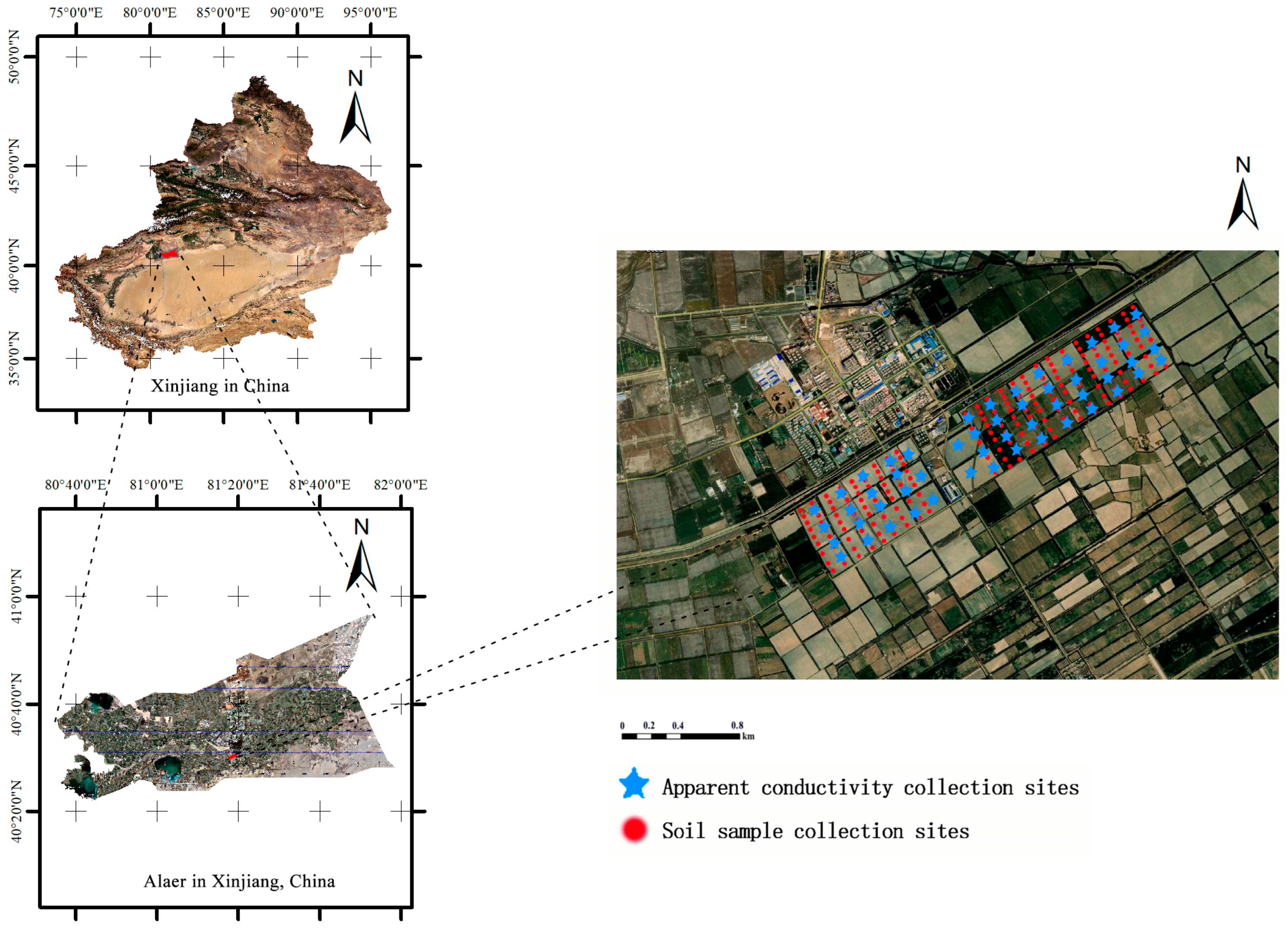
2.1. Overview

The studied area is located in the 12th regiment of Alar Reclamation District, Xinjiang Uygur Autonomous Region. The area under jurisdiction is 524.8 square kilometers, with 21,200 hectares of arable land, including 240,000 mu for cotton and 78,000 mu for forestry and fruit industries. The altitude of the area is 990~1040 m, the groundwater level is between 1.4~1.7 m, and the rainfall is mainly in June, July, and August, with an evapotranspiration ratio of 40:1, which is typical of an extreme aridity area, and the area is rich in light and heat resources, with a frost-free period of 206–220 days. The geographical distribution of the study area is between 81°29′–81°35′ E and 40°48′–40°51′ N, with a total area of 4.45 km² (Figure 1), and the soil type is sandy loam, and the main crop is cotton.

2.2. Soil Sample Collection and Processing

In March 2022, we collected 75 soil samples from the study area using a “random sampling” method at depths of 0–20 cm. The coordinates and latitude and longitude of all sampling points were recorded by a cell phone’s GPS. At the time of sampling, the cotton in the farmland had been harvested. The soil samples were sealed, labeled, sent back to the laboratory, placed in a ventilated location, dried naturally, ground, and sieved. Subsequently, the soil organic matter content, total nitrogen, total phosphorus, total potassium, and pH were, respectively, measured by potassium dichromate volumetric method, Kjeldahl method, acid soluble-molybdenum antimony anti-colorimetric method, sodium hydroxide fusion method, and PHS-3C pH meter [22].

2.3. Principal Component Analysis

Before setting up partitions for the fields, data dimensionality reduction was first performed by using principal component analysis (PCA), which is a multivariate data analysis method that can transform the original data into a set of mutually independent principal component variables through a linear transformation [23]. Thereby, it simplifies the data structure, reduces dimensionality, and retains key information in the data. The basic idea of the method is to maximize the data variance in a new coordinate system, because the variance reflects the degree of data variability. The dimensionality was reduced through principal component analysis; the key information of the data, i.e., the information features of variables with high variance, can be retained. PCA is widely used in data pre-processing, data compression, feature extraction, and visualization. In machine learning, PCA is a commonly used technique for data dimensionality reduction, feature extraction, and model simplification.

2.4. Fuzzy c-Means Clustering

The basic idea of fuzzy c-mean clustering (FCM) is to find an objective function that can be minimized within a given number of iterations. The biggest advantage of FCM is that it can make full use of sampled data to improve the clustering accuracy. The most commonly used objective function is shown in Equation (1) [24].

$$J_m(U,V)=\sum _{k=1}^n\sum _{i=1}^c{\left(u_{ik}\right)}^m{\left(d_{ik}\right)}^2,$$

(1)

where $n$ and $c$ denote the number of data and the number of categories, respectively. $m$ is the fuzzy weighting index $(1\le m\le \mathsf{\infty })$, which controls the number of sharing data between different categories; when $m$ approaches infinity, the number of shared data increases, and the final classification becomes less obvious. When $m=1$, hard clustering occurs, i.e., there is no data sharing. $u_{ik}(1\le i\le c,1\le k\le n)$ denotes that the $k$th sample $X_k$ in the data matrix $X\in R^{n\times c}$ ($X\in R^{n\times c}$ represents a data matrix belonging to n rows and c columns) belongs to the affiliation value of the $i$th clustering center $v_i$ in the clustering center matrix $V$. $U$ is the affiliation matrix. ${d_{ik}}^2$ is equal to the square of the distance between $x_k$ and $v_i$ on the eigenvector.

$$v_i^b=\frac{{\sum }_{k=1}^n{\left(u_{ik}\right)}^m{x}_k}{{\sum }_{k=1}^n{\left(u_{ik}\right)}^m},$$

(2)

$$u_{ik}^{ \left(b+1\right)}={\left[\sum _{j=1}^c{\left(\frac{d_{ik}^{ \left(b\right)}}{d_{jk}^{ \left(b\right)}}\right)}^{\frac{2}{m-1}}\right]}^{-1}.$$

(3)

The fuzzy c-means clustering algorithm achieves classification through an iterative optimization process. The first step is the initialization of the affiliation matrix $U$. Then, according to Equation (2), $c$ cluster centers are calculated, and from these cluster centers, the affiliation values of each data point in the class are calculated (see Equation (3)), the affiliation matrix is adjusted, and the new $c$ cluster centers are calculated based on the adjusted affiliation matrix, and the new $c$ cluster centers are compared.

The affiliation matrix was adjusted, the new c clustering centers were calculated based on the adjusted affiliation matrix, the changes in the clustering centers were compared, and the iterative computation was stopped if the amount of change between the two loops was less than the preset threshold, otherwise, the previous steps were repeated until the change in the clustering centers was less than the set threshold.

2.5. Clustering Validity Test

In the clustering process, there is often a problem of determining the right number of clusters. Good clustering should be as clear as possible. In order to obtain the appropriate number of clusters and evaluate the clustering effect, fuzzy performance index and normalized classification entropy are used to determine the number of clusters and evaluate the clustering effect.

The fuzzy performance index (FPI) is used to measure the separation of the data matrix $X$ between fuzzy $c$ partitions, and it is defined as the following [25]:

$$\mathrm{F}\mathrm{P}\mathrm{I}=1-\frac{c}{\left(c-1\right)}\left[1-\sum _{k=1}^n\sum _{i=1}^c\frac{{\left(u_{ik}\right)}^2}{n}\right],$$

(4)

FPI is the average of the minimum values in the matrix to which each sample belongs. The FPI value decreases as the number of clusters increases, because the compactness and separation of the clusters can be increased by increasing the number of clusters. Therefore, the FPI can be used to estimate the effect of different numbers of clusters and to select the optimal number of clusters.

Normalized classification entropy (NCE) is a measure of the decomposition of the data matrix X in the fuzzy c-partition. Among them, the classification entropy (H) can be calculated by using the following equation [25]:

$$H(U;c)=-\frac{{\sum }_{k=1}^n{\sum }_{i=1}^c{u}_{ik}{\log }_a\left(u_{ik}\right)}{n},$$

(5)

$$\mathrm{N}\mathrm{C}\mathrm{E}=\frac{H\left(U;c\right)}{\left[1-\left(\frac{c}{n}\right)\right]}.$$

(6)

Any positive integer $a$ can be taken as the base, and the value of H ranges from 0 to ${\log }_a\left(c\right)$. Because H is equal to 0 for c equal to 1 or n. Bezdek summarized the definition of normalized classification moisture by analyzing the classification moisture and found that the smaller the $\mathrm{N}\mathrm{C}\mathrm{E}$, the larger the decomposition capacity of the corresponding fuzzy c-partition and the better the clustering effect [26].

Descriptive statistical analysis, correlation analysis, principal component analysis, and analysis of variance (ANOVA) of the measured data of the soil samples were processed in SPSS 25.0 software; principal component plotting and partitioning maps were processed using ArcGIS 10.8 software; and FCM cluster analysis was carried out in MZA, the software for managing partitions. In order to find out the optimal number of partitions, 2, 3, 4, 5, and 6 categories were generated, and the values of FPI and NCE for each category were calculated and compared, and the optimal number of partitions was the one that was minimized when both FPI and NCE were minimized at the same time [27].

3. Results and Analysis

3.1. Descriptive Statistics of Soil Properties

The descriptive statistics of the soil properties at the 75 sampling sites are presented in

Table 1. Statistical characteristic values of soil properties ($n$ = 75).

Soil Properties	Max.	Min.	Average	S.D.	C.V.	Skewness	Kurtosis	K-S
Apparent conductivity (Eca) mS m−1	14.56	0.38	4.37	2.71	0.62	0.28	0.55	0.69
Organic matter g kg−1	26.37	4.68	18.35	3.76	0.20	−0.36	0.76	0.67
Total nitrogen g kg−1	7.83	0.11	0.94	0.23	0.24	0.98	3.77	0.44
Total phosphorus g kg−1	2.28	0.46	1.13	0.42	0.37	0.67	0.83	0.65
Total potassium g kg−1	23.41	8.36	16.77	2.22	0.13	−0.17	1.13	0.73
pH	8.74	7.88	8.29	0.29	0.03	−0.29	−0.87	0.47

C.V. is the coefficient of variation, S.D. is the standard deviation, and K-S is the value of the Kolmogorov–Smirnov test.

. Although the mean value of the soil conductivity was only 4.37 mS m⁻¹, it was highly variable, with an extreme value of 14.56 mS m⁻¹. From Table 1, it can be seen that the study area is lightly salinized, the mean value of the soil organic matter is at a moderate level, the total nitrogen and phosphorus content of the soil is at a low level, and the total potassium content is at a high level [28]. In addition, according to the observation of the coefficient of variation, all the soil properties are at a moderate level of variability, except for the weak variability of pH (C.V. ≥ 1, 0.1 ≤ C.V. < 1, C.V. < 0.1 are, respectively, strong variability, moderate variability, and weak variability) [29]. The one-sample Kolmogorov–Smirnov method (p < 5%, two-tailed test) was used to test the normality of each soil attribute, and the results showed that the attributes conformed to the characteristics of normal distribution. Overall, the soils in the study area had a low organic matter content and nutrient content, high salinity, and high alkalinity.

3.2. Correlation Analysis of Soil Properties

The matrix of correlation coefficients between the soil properties is presented in

Table 2. Plot of correlation coefficients of soil properties ($n$ = 75).

Soil Properties	Eca	Organic Matter	Total Nitrogen	Total Phosphorus	Total Potassium	pH
Eca	1	0.279	0.271	0.223	−0.084	−0.512 **
Organic matter	0.279	1	0.713 **	0.224	0.461 **	−0.097
Total nitrogen	0.271	0.713 **	1	0.406 **	0.507 **	−0.188
Total phosphorus	0.223	0.224	0.406 **	1	0.374 *	−0.277
Total potassium	−0.084	0.461 **	0.507 **	0.374 *	1	0.137
pH	−0.512 **	−0.097	−0.188	−0.277	0.137	1

* p < 5%. ** p < 1%.

. The results showed that there was a significant negative correlation between the soil Eca and pH in the study area, while there was no significant correlation between the soil Eca and the organic matter and nutrient content. Organic matter had a significant positive correlation with the total nitrogen and potassium, while there was no significant correlation with the other soil properties. The total nitrogen showed a significant positive correlation with the total phosphorus and total potassium and no significant correlation with the other soil properties. The total phosphorus was significantly positively correlated with the total potassium and negatively correlated with pH. In addition, there was a positive correlation between the total potassium and total phosphorus.

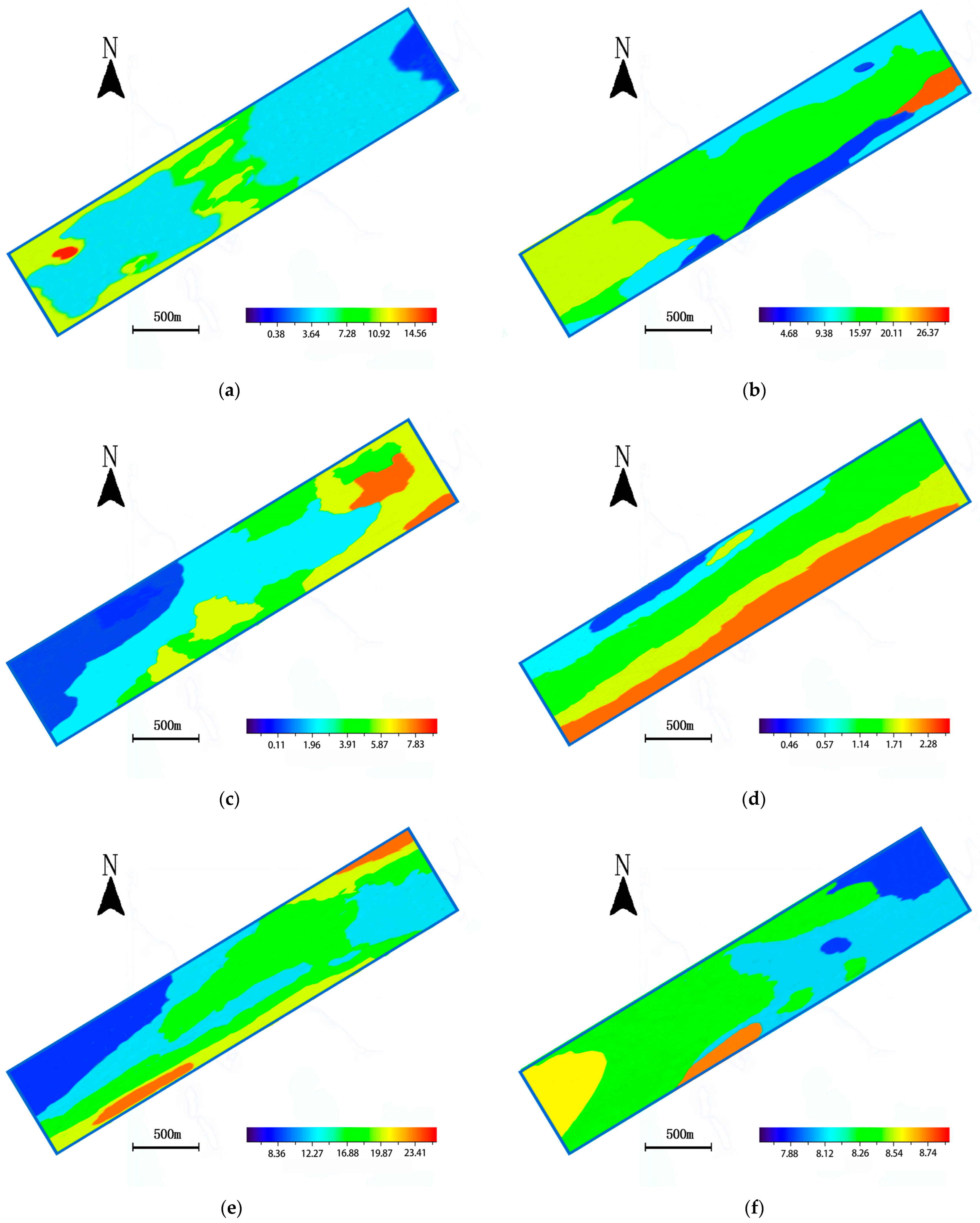
3.3. Spatial Distribution Characteristics of Soil Properties

Figure 2 shows the spatial distribution of the six soil properties after conducting the ordinary kriging analysis. From the interpolation results, the kriging interpolation method smoothed the data of each soil attribute, making the large values lower and the small values higher, thus reducing the abruptness of the soil attribute data. From Figure 2, it can be seen that each soil attribute shows a more obvious spatial structure, and each attribute shows different distribution characteristics in space. The soil conductivity was higher in the southwest and lower in the northeast; the organic matter content was relatively lower in the center and higher in the southwest; the total nitrogen was lower in the northwest and significantly higher in other areas; the distribution of the total phosphorus was significantly higher in the southeast than in the northwest, and showed a decreasing trend from southwest to northeast; the overall distribution of the total potassium showed a higher trend in the center, lower in the northwest, balanced in the center, and higher in the northeast and southwest. The overall distribution of the total potassium showed a trend of balance in the center, low in the southeast and high in the northwest.

3.4. Principal Component Analysis of Soil Properties

In view of the six different soil attributes, the corresponding raster data have some correlation in the cluster analysis, and there is a certain degree of overlap among the information reflected by different attributes. Therefore, firstly, by using the principal component analysis, the useful information in the original raster images corresponding to the six soil attributes is concentrated in the new principal component images, and a smaller number of principal component images are selected, by which the dimensionality of the data can be reduced and thus the raster image information can be highlighted. Subsequently, the results of the principal component analysis were analyzed by fuzzy c-mean clustering. The six soil attributes were analyzed using principal component analysis (PCA), The Kaiser–Meyer–Olkin (KMO) and Barlett tests were first performed on the raw data and the results are shown in

Table 3. KMO and Bartlett test.

Test Methods	Indexs	Value
KMO quantity of sample suitability	/	0.787
Bartlett sphericity test	Approximate chi-squared	996.443
	Degrees of freedom	20
	Significance	0

. The PCA shown here is a rotated PCA and the rotation method is the maximum variance method. While components with eigenvalues greater than 1 were retained, a total of three principal components were extracted in this study process, and the cumulative variance contribution reached 87.57% with high confidence. The eigenvalues of the different principal components and their variance contribution rates are given in

Table 4. Eigenvalues and contribution rates.

PCA	Eigenvalue	Contribution Rate
PC1	2.21	43.29%
PC2	1.49	27.16%
PC3	1.13	17.12%
Totals		87.57%

, while the corresponding load matrices of the different principal components are illustrated in

Table 5. Principal component loading matrix.

Soil Properties	PC1	PC2	PC3	Commonality
Eca	0.41	−0.74	−0.03	0.72
Organic matter	0.61	−0.03	0.61	0.71
Total nitrogen	0.84	−0.07	0.32	0.82
Total phosphorus	0.61	−0.14	−0.52	0.69
Total potassium	0.81	0.39	−0.51	0.81
pH	−0.29	0.61	0.26	0.67

.

In Table 4, the variance contribution of the first principal component is 43.29%, and the loadings of the first principal component on the total N and total K are as high as 0.84 and 0.81, respectively, which are significantly higher than the loadings corresponding to the other soil attributes, and the first principal component mainly reflects the information on the total N and total K. Similarly, the variance contribution of the second principal component is 27.16%, which mainly portrays the information related to the conductivity and pH, and the variance contribution of the third principal component is 17.12%, which mainly reflects the information on the organic matter, total phosphorus, and total K. Similarly, the variance contribution of the second principal component is 27.16%, which mainly portrayed the information related to the conductivity and pH, and the variance contribution of the third principal component is 17.12%, which mainly reflected the information related to the organic matter, total phosphorus, and total potassium.

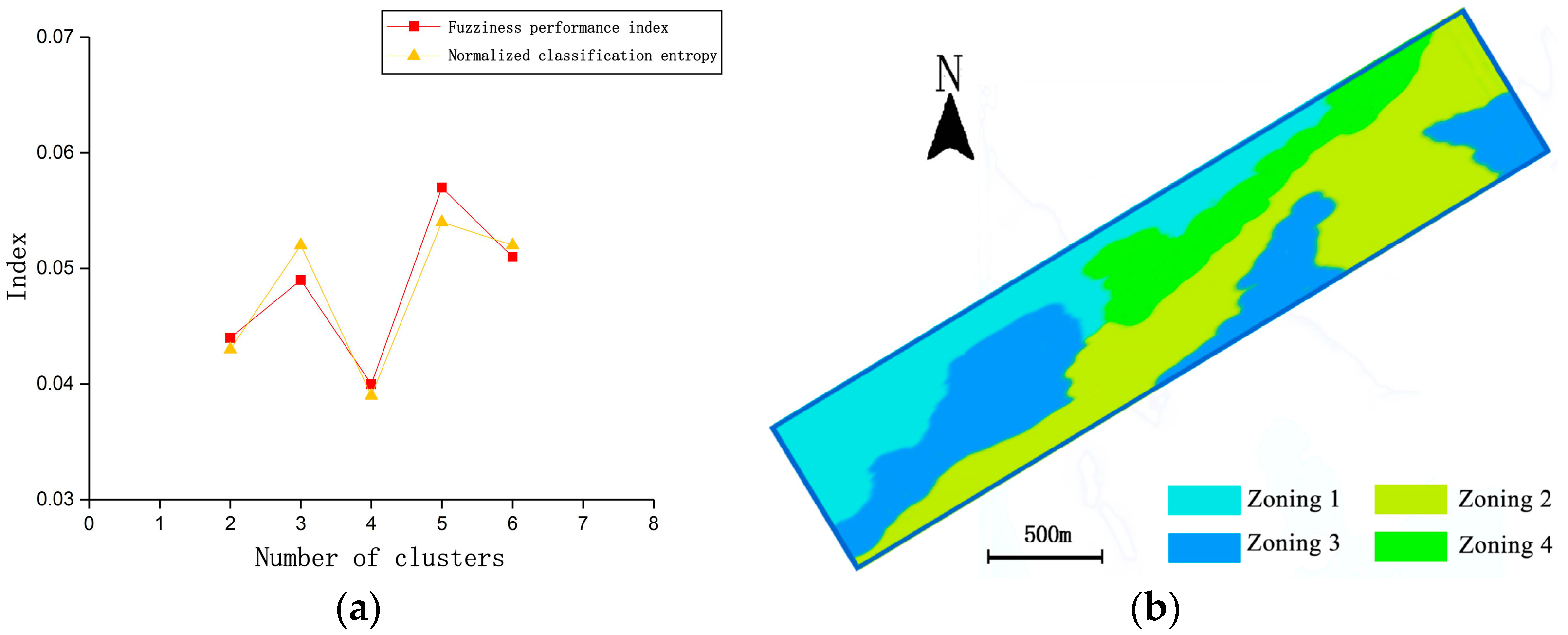
3.5. FCM Clustering Analysis and Managed Partitioning

The collected sample point data were analyzed using the FCM algorithm by taking the maximum number of iterations as 200, convergence threshold as 0.001, and fuzzy weighted index as 1.7. To determine the optimal number of categories, six clusters were used as management zones and their maximum actual usage was considered. Two quantitative evaluation indices, FPI and NCE, were used as the indicators of the optimal number of categories, as shown in Figure 3a. The optimal number of categories for a given category is indicated when both the evaluation indices for that category are minimized. As shown in Figure 3a, the FPI and NCE do not show a monotonous increasing or decreasing pattern as the number of subdivisions increases, but they have a similar trend, with the smallest values when the number of categories is four. Therefore, for this study area, the optimal number of partitions is four. Figure 3b shows the corresponding map of the management partitions when the number of partitions is four.

3.6. Managing Partition Accuracy Checks

In order to accurately evaluate whether the four management partitions can reasonably and quantitatively express the spatial variation in the various soil properties, all the soil sample points were divided into four management partitions. Among all 75 sampling points, 17 sample points were classified as partition 1, 19 sample points were classified as partition 2, 18 sample points were classified as partition 3, and the remaining 21 sample points were classified as partition 4. By employing ANOVA, the differences in the attributes of different soils were examined among the different management sub-areas. The descriptive statistics of the ANOVA results for each soil attribute among the different management zones are shown in

Table 6. Results of descriptive statistics of soil properties in each partition.

Management Zone	Variables	ECa (mS m−1)	Organic Matter (g kg−1)	Total Nitrogen (g kg−1)	Total Phosphorus (g kg−1)	Total Potassium (g kg−1)	pH
Zoning 1 (n = 17)	Min.	1.38	4.68	0.11	0.46	8.36	7.88
	Max.	14.56	15.9	4.23	0.97	19.46	8.74
	S.D.	1.09	2.89	0.13	0.09	1.67	0.35
	C.V.	0.19	0.26	0.15	0.21	0.12	0.04
Zoning 2 (n = 19)	Min.	0.38	7.96	0.28	0.77	11.36	7.92
	Max.	6.79	26.37	7.83	2.28	23.41	8.13
	S.D.	0.81	1.77	0.19	0.18	1.36	0.76
	C.V.	0.27	0.09	0.08	0.10	0.07	0.09
Zoning 3 (n = 18)	Min.	0.52	5.37	0.19	0.55	13.27	7.89
	Max.	11.32	19.77	4.97	1.84	18.46	8.63
	S.D.	1.16	2.22	0.23	0.18	1.77	0.55
	C.V.	0.23	0.17	0.14	0.24	0.12	0.07
Zoning 4 (n = 21)	Min.	0.79	6.32	0.23	0.63	9.74	7.94
	Max.	8.34	16.32	5.22	1.76	21.33	8.52
	S.D.	2.13	2.89	0.57	0.11	1.67	0.47
	C.V.	0.29	0.26	0.31	0.12	0.10	0.06
Significant level	p	0.03 *	0.02 *	0.02 *	0.00 **	0.00 **	0.79

* p < 5%. ** p < 1%. Zoning 1 has a high salinity and lowest nutrient content; Zoning 2 has the lowest degree of salinity and the highest nutrient content; Zoning 3 has a high salinity and low nutrient content; Zoning 4 has the highest salinity and low affective content; and all four zonings are mildly saline.

and the means comparisons are displayed in

Table 7. Mean values for soils in each subzone.

Management Zone	Variables	ECa (mS m−1)	Organic Matter (g kg−1)	Total Nitrogen (g kg−1)	Total Phosphorus (g kg−1)	Total Potassium (g kg−1)	pH
Zoning 1	Average	5.76	11.32	0.86	0.42	14.31	8.27
Zoning 2	Average	2.98	19.28	2.34	1.84	19.23	8.02
Zoning 3	Average	5.11	13.22	1.67	0.76	15.17	8.31
Zoning 4	Average	7.23	11.22	1.83	0.93	16.41	8.14

.

From Table 6, it can be seen that the soil’s total phosphorus and total potassium differed highly significantly at the p < 1% level, while the soil’s electrical conductivity, organic matter, and total nitrogen differed significantly at the p < 5% probability level among the management zones. From Table 7, a comparison of the mean values of each soil attribute for the four management zones revealed that management zone 2 had the highest level of soil fertility and the lowest soil electrical conductivity. For the favorable indicators of crop yield enhancement such as the soil organic matter, total nitrogen, total phosphorus, and total potassium, zone 2 was significantly better than the other three zones, while the unfavorable indicators of crop yield enhancement such as the soil electrical conductivity were significantly lower in zone 2 than in the other three zones. The statistical data of the four zones proved the existence of the soil attributes’ differences among the management zones. The indicators of the soil fertility levels, such as the total phosphorus and total potassium, were significantly higher in management sub-area 2 than in the other three management sub-areas, which is consistent with the findings of Fu et al. [30]. In the case of essentially the same field management practices, this may be related to a variety of factors such as the soil texture, pore structure, aggregate stability, and even soil moisture status in the four sub-areas [31].

Defining specific field management zones is based on the comprehensive analysis of multiple spatial aspects, specifically soil physical and chemical properties, topographic attributes, remote sensing images, crop canopy images, and yield maps. The stability and predictability of this information is important to delineate crop productivity management partitions. In this study, we used principal component analysis and the FCM clustering method to construct a soil attribute library with data on a total of six soil attributes to delineate crop productivity management partitions in cotton fields. Given that data on the soil conductivity, organic matter, and other related attributes have a great impact on agricultural production and crop economic efficiency, it is feasible to use these soil attribute data to partition the study area for management. In addition, the selected study area has been managed for many years in the field, and the topography is flat and small, thus the topographic and elevation data are not involved in this paper. The results of the management zoning investigation in this paper can provide some reference basis for fertilizer management before and during sowing, etc. In future research, the introduction of richer basic data sources can be considered to improve the management zoning work to better guide agricultural production and thus enhance economic efficiency.

4. Conclusions

(1)

The soils in the study area were mildly saline, low in soil organic matter and total nitrogen, medium in total phosphorus, and high in conductivity, total potassium, and pH. The variability of all the soil properties was moderate except for pH, which was weak.

(2)

The interpolation results of the soil attributes showed that the six soil attributes have an obvious spatial structure, but different attributes have large differences in spatial distribution.

(3)

The results of the principal component analysis showed that the six soil attributes were classified into three principal components, and based on this, the study area was divided into four management zones using the FCM cluster analysis and two quantitative evaluation indicators, FPI and NCE.

(4)

The results of the ANOVA showed significant differences in soil properties such as the soil conductivity, organic matter, and soil nutrients in different management zones. Therefore, the FCM cluster analysis and different soil attributes can be used to determine the management zoning of farmland in the study area.

References

1. Abuelgasim, A.; Ammad, R. Mapping soil salinity in arid and semi-arid regions using landsat 8 oli satellite data. Remote Sens. Appl. Soc. Environ. 2019, 13, 415–425. [Google Scholar] [CrossRef]
2. Khan, M.; Almazah, M.M.; EIlahi, A.; Niaz, R.; Al-Rezami, A.; Zaman, B. Spatial interpolation of water quality index based on ordinary kriging and universal kriging. Geomat. Nat. Hazards Risk 2023, 14, 2190853. [Google Scholar] [CrossRef]
3. Li, J.; Pu, L.; Han, M.; Zhu, M.; Zhang, R.; Xiang, Y. Soil salinization research in china: Advances and prospects. J. Geogr. Sci. 2014, 24, 943–960. [Google Scholar] [CrossRef]
4. Hopmans, J.W.; Qureshi, A.; Kisekka, I.; Munns, R.; Grattan, S.; Rengasamy, P.; Ben-Gal, A.; Assouline, S.; Javaux, M.; Minhas, P.; et al. Critical knowledge gaps and research priorities in global soil salinity. Adv. Agron. 2021, 169, 1–191. [Google Scholar]
5. Xiao, C.; Li, M.; Fan, J.; Zhang, F.; Li, Y.; Cheng, H.; Li, Y.; Hou, X.; Chen, J. Salt leaching with brackish water during growing season improves cotton growth and productivity, water use efficiency and soil sustainability in southern Xinjiang. Water 2021, 13, 2602. [Google Scholar] [CrossRef]
6. Al-Ali, Z.; Bannari, A.; Rhinane, H.; El-Battay, A.; Shahid, S.A.; Hameid, N. Validation and comparison of physical models for soil salinity mapping over an arid landscape using spectral reflectance measurements and landsat-oli data. Remote Sens. 2021, 13, 494. [Google Scholar] [CrossRef]
7. Kumar, N.; Singh, S.K.; Pandey, H. Drainage morphometric analysis using open access earth observation datasets in a drought-affected part of bundelkhand, india. Appl. Geomat. 2018, 10, 173–189. [Google Scholar] [CrossRef]
8. Chen, H.; Zhao, G.; Li, Y.; Wang, D.; Ma, Y. Monitoring the seasonal dynamics of soil salinization in the yellow river delta of china using landsat data. Nat. Hazards Earth Syst. Sci. 2019, 19, 1499–1508. [Google Scholar] [CrossRef]
9. Komarov, S.; Antropov, D.; Varlamov, A.; Galchenko, S.; Zhdanova, R. Zoning as a tool of land management. IOP Conf. Ser. Earth Environ. Sci. 2019, 350, 012060. [Google Scholar] [CrossRef]
10. Zhang, H.; Liang, X.; Chen, H.; Shi, Q. Spatio-temporal evolution of the social-ecological landscape resilience and management zoning in the loess hill and gully region of china. Environ. Dev. 2021, 39, 100616. [Google Scholar] [CrossRef]
11. Moharana, P.; Jena, R.; Pradhan, U.; Nogiya, M.; Tailor, B.; Singh, R.; Singh, S. Geostatistical and fuzzy clustering approach for delineation of site-specific management zones and yield-limiting factors in irrigated hot arid environment of india. Precis. Agric. 2020, 21, 426–448. [Google Scholar] [CrossRef]
12. Yasir, M.; Sheng, H.; Fan, H.; Nazir, S.; Niang, A.J.; Salauddin, M.; Khan, S. Automatic coastline extraction and changes analysis using remote sensing and gis technology. IEEE Access 2020, 8, 180156–180170. [Google Scholar] [CrossRef]
13. Perron, I.; Cambouris, A.N.; Chokmani, K.; Gutierrez, M.F.V.; Zebarth, B.J.; Moreau, G.; Biswas, A.; Adamchuk, V. Delineating soil management zones using a proximal soil sensing system in two commercial potato fields in new brunswick, Canada. Can. J. Soil Sci. 2018, 98, 724–737. [Google Scholar] [CrossRef]
14. Metwally, M.S.; Shaddad, S.M.; Liu, M.; Yao, R.-J.; Abdo, A.I.; Li, P.; Jiao, J.; Chen, X. Soil properties spatial variability and delineation of site-specific management zones based on soil fertility using fuzzy clustering in a hilly field in jianyang, sichuan, china. Sustainability 2019, 11, 7084. [Google Scholar] [CrossRef]
15. Shukla, M.K.; Sharma, P. Fuzzy k-means and principal component analysis for classifying soil properties for efficient farm management and maintaining soil health. Sustainability 2023, 15, 13144. [Google Scholar] [CrossRef]
16. Jaynes, D.; Kaspar, T.; Colvin, T.; James, D. Cluster analysis of spatiotemporal corn yield patterns in an iowa field. Agron. J. 2003, 95, 574–586. [Google Scholar] [CrossRef]
17. Techen, A.-K.; Helming, K.; Brüggemann, N.; Veldkamp, E.; Reinhold-Hurek, B.; Lorenz, M.; Bartke, S.; Heinrich, U.; Amelung, W.; Augustin, K.; et al. Soil research challenges in response to emerging agricultural soil management practices. Adv. Agron. 2020, 161, 179–240. [Google Scholar]
18. Gavioli, A.; de Souza, E.G.; Bazzi, C.L.; Schenatto, K.; Betzek, N.M. Identification of management zones in precision agriculture: An evaluation of alternative cluster analysis methods. Biosyst. Eng. 2019, 181, 86–102. [Google Scholar] [CrossRef]
19. Zhang, Y.; Li, Y.; Sun, J.; Huang, G. Optimizing water resources allocation and soil salinity control for supporting agricultural and environmental sustainable development in central asia. Sci. Total Environ. 2020, 704, 135281. [Google Scholar] [CrossRef]
20. Montanarella, L.; Panagos, P. The relevance of sustainable soil management within the european green deal. Land Use Policy 2021, 100, 104950. [Google Scholar] [CrossRef]
21. Asfaw, E.; Suryabhagavan, K.; Argaw, M. Soil salinity modeling and mapping using remote sensing and gis: The case of wonji sugar cane irrigation farm, Ethiopia. J. Saudi Soc. Agric. Sci. 2018, 17, 250–258. [Google Scholar] [CrossRef]
22. Pansu, M. Handbook of Soil Analysis; Springer: Berlin/Heidelberg, Germany, 2006. [Google Scholar]
23. Uddin, M.P.; Mamun, M.A.; Hossain, M.A. PCA-based feature reduction for hyperspectral remote sensing image classification. IETE Tech. Rev. 2021, 38, 377–396. [Google Scholar] [CrossRef]
24. Rahbar, A.; Vadiati, M.; Talkhabi, M.; Nadiri, A.A.; Nakhaei, M.; Rahimian, M. A hydrogeochemical analysis of groundwater using hierarchical clustering analysis and fuzzy c-mean clustering methods in arak plain, Iran. Environ. Earth Sci. 2020, 79, 1–17. [Google Scholar] [CrossRef]
25. Damian, J.M.; Santi, A.L.; Fornari, M.; Da Ros, C.O.; Eschner, V.L. Monitoring variability in cash-crop yield caused by previous cultivation of a cover crop under a no-tillage system. Comput. Electron. Agric. 2017, 142, 607–621. [Google Scholar] [CrossRef]
26. Bezdek, J.C. Pattern Recognition with Fuzzy Objective Function Algorithms; Springer Science & Business Media: Berlin/Heidelberg, Germany, 2013. [Google Scholar]
27. Fridgen, J.J.; Kitchen, N.R.; Sudduth, K.A.; Drummond, S.T.; Wiebold, W.J.; Fraisse, C.W. Management zone analyst (MZA) software for subfield management zone delineation. Agron. J. 2004, 96, 100–108. [Google Scholar]
28. Zaman, M.; Shahid, S.A.; Heng, L.; Shahid, S.A.; Zaman, M.; Heng, L. Introduction to soil salinity, sodicity and diagnostics techniques. In Guideline for Salinity Assessment, Mitigation and Adaptation Using Nuclear and Related Techniques; Springer International Publishing: Berlin/Heidelberg, Germany, 2018; pp. 1–42. [Google Scholar]
29. Wei, Y.; Ding, J.; Yang, S.; Wang, F.; Wang, C. Soil salinity prediction based on scale-dependent relationships with environmental variables by discrete wavelet transform in the tarim basin. Catena 2021, 196, 104939. [Google Scholar] [CrossRef]
30. Fu, Q.; Wang, Z.; Jiang, Q. Delineating soil nutrient management zones based on fuzzy clustering optimized by pso. Math. Comput. Model. 2010, 51, 1299–1305. [Google Scholar] [CrossRef]
31. Shaver, T.; Peterson, G.; Ahuja, L.R.; Westfall, D. Soil sorptivity enhancement with crop residue accumulation in semiarid dryland no-till agroecosystems. Geoderma 2013, 192, 254–258. [Google Scholar] [CrossRef]
Figure 1. Geographical location map of the studied area.
Agriculture 14 00003 g001
Figure 2. Spatial distribution of soil properties. (a) ECa (mS/m. (b) Organic matter (g/kg). (c) Total Nitrogen (g/kg). (d) Total Phosphorus (g/kg). (e) Total Potassium (g/kg). (f) pH.
Agriculture 14 00003 g002
Figure 3. Results of management partitioning based on six soil attributes. (a) Classification and evaluation indicators. (b) Distribution maps of the resultant management zones.
Agriculture 14 00003 g003