
Partitioning Evapotranspiration in a Cotton Field under Mulched Drip Irrigation Based on the Water-Carbon Fluxes Coupling in an Arid Region in Northwestern China


Abstract
1. Introduction
2. Materials and Methods
2.1. Study Area
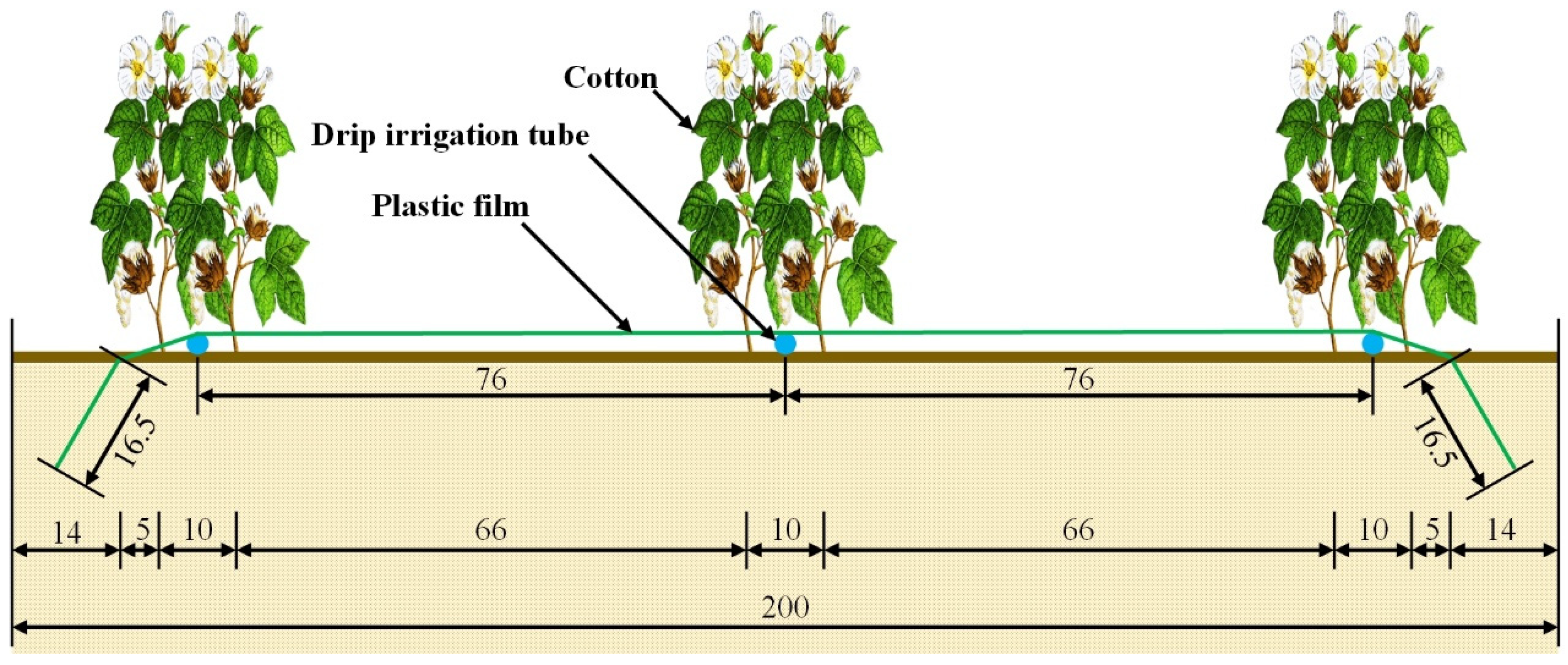
2.2. Cotton Cultivation Pattern and Management
2.3. Measurements
2.4. EC System
2.4.1. Correct Fluxes Data
2.4.2. Select Typical Day
2.4.3. Calculate GPP
2.4.4. Partition ET Based on Water–Carbon Flux Coupling
3. Results
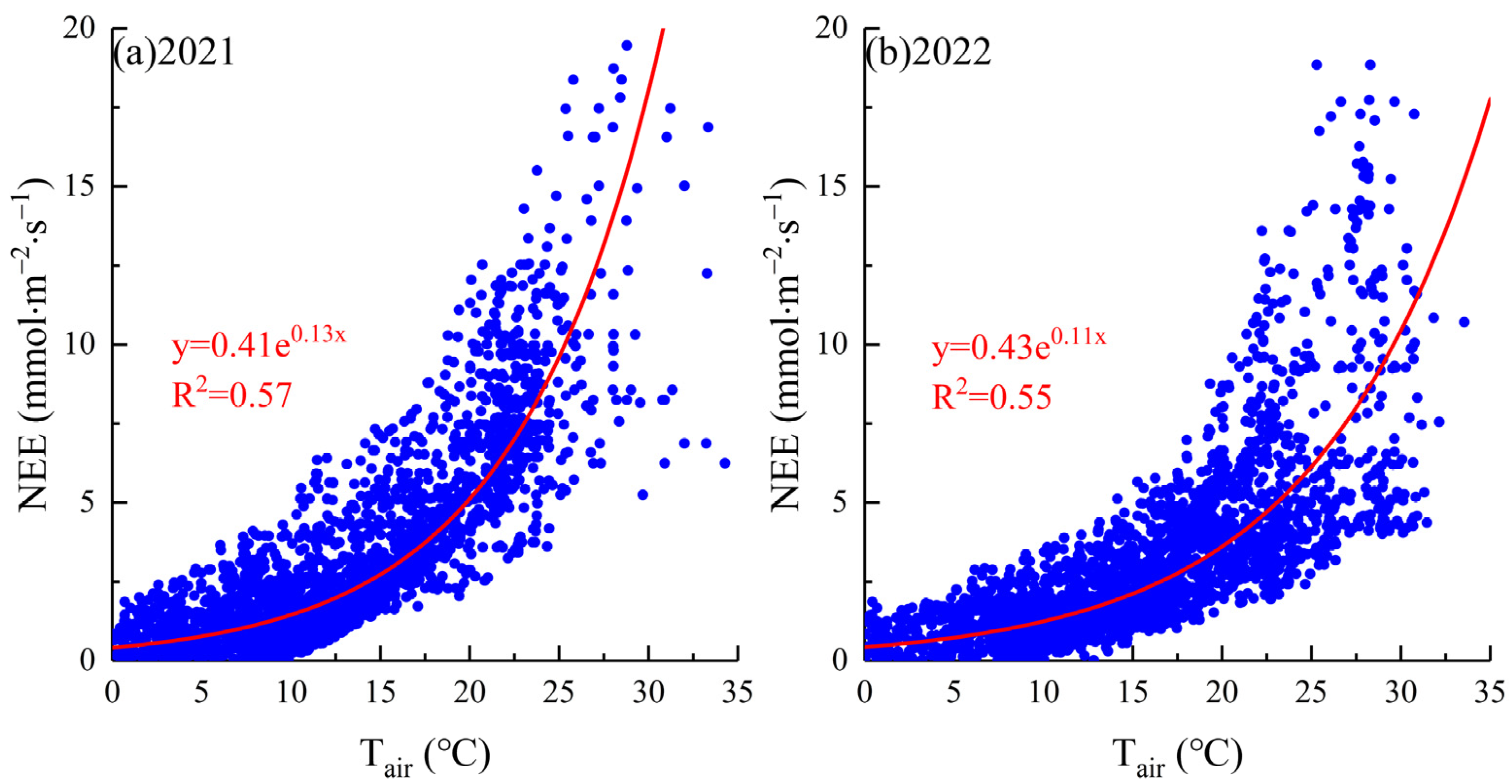
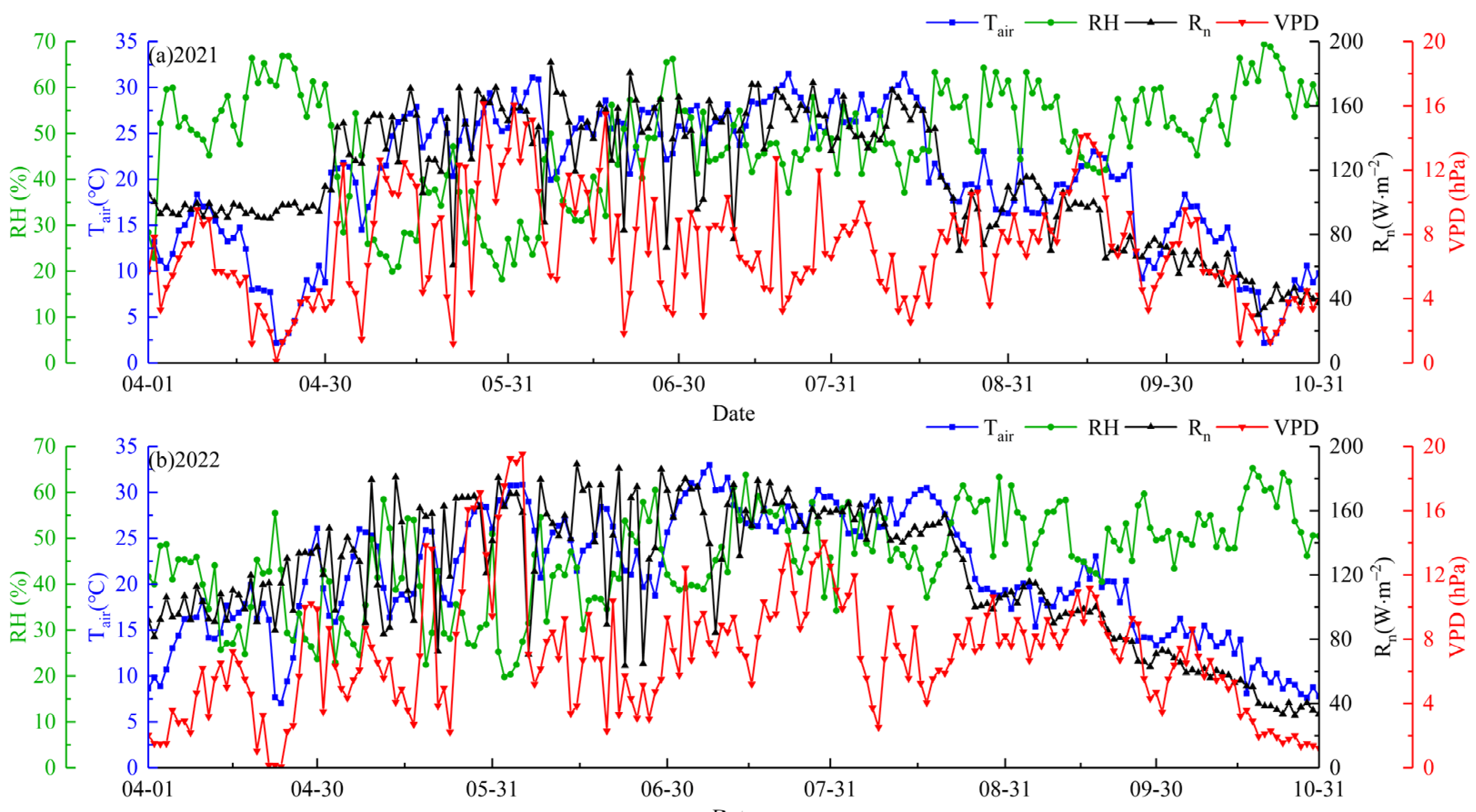
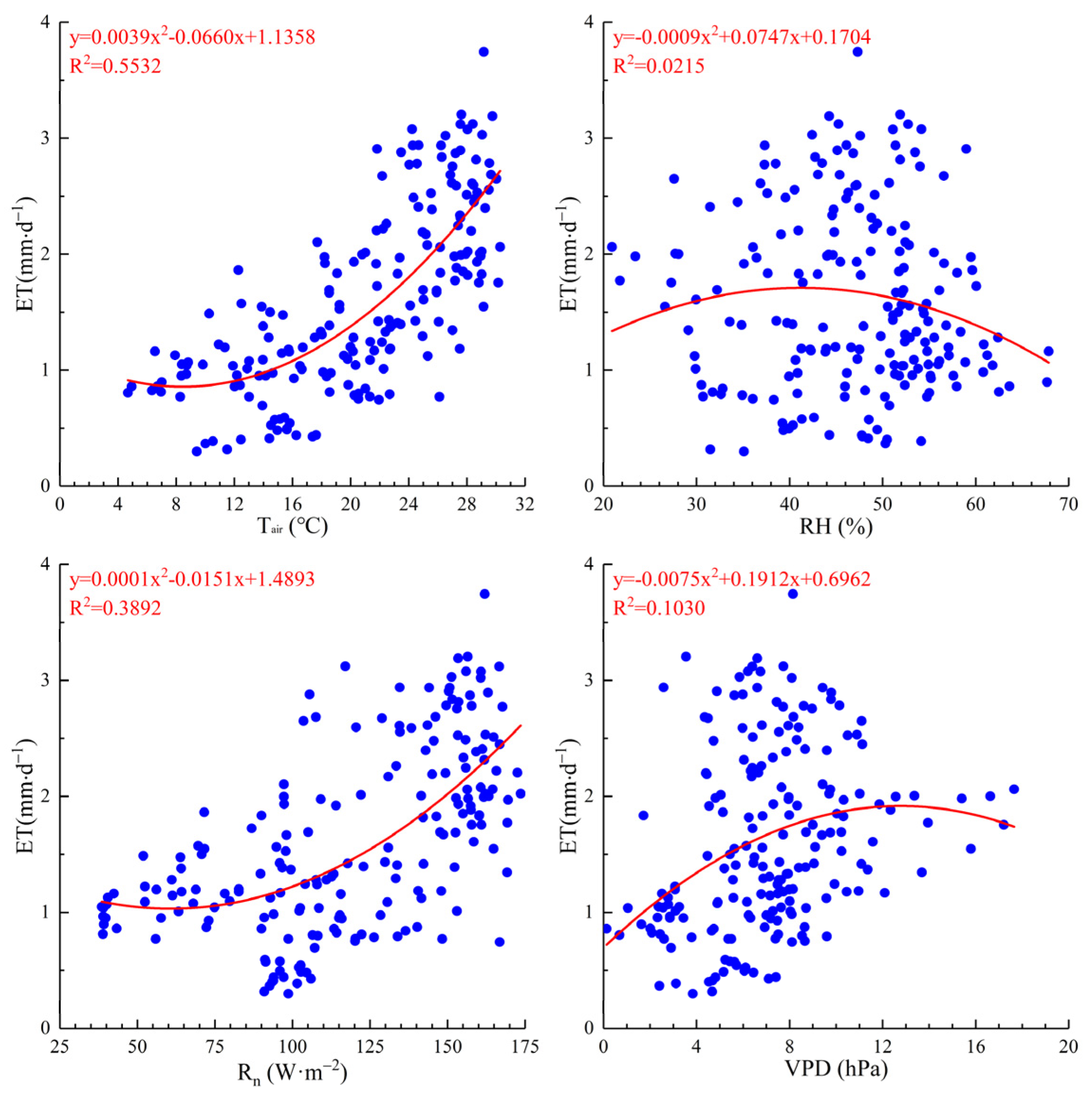
3.1. Environmental Factors
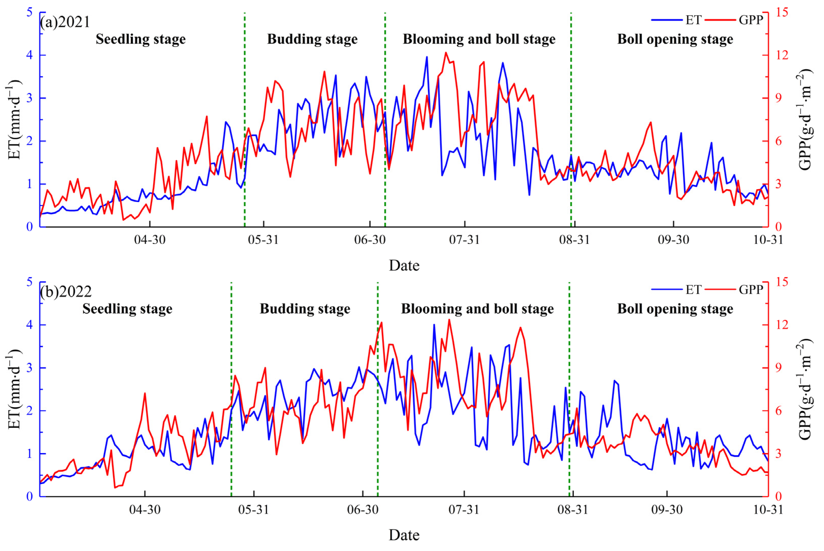
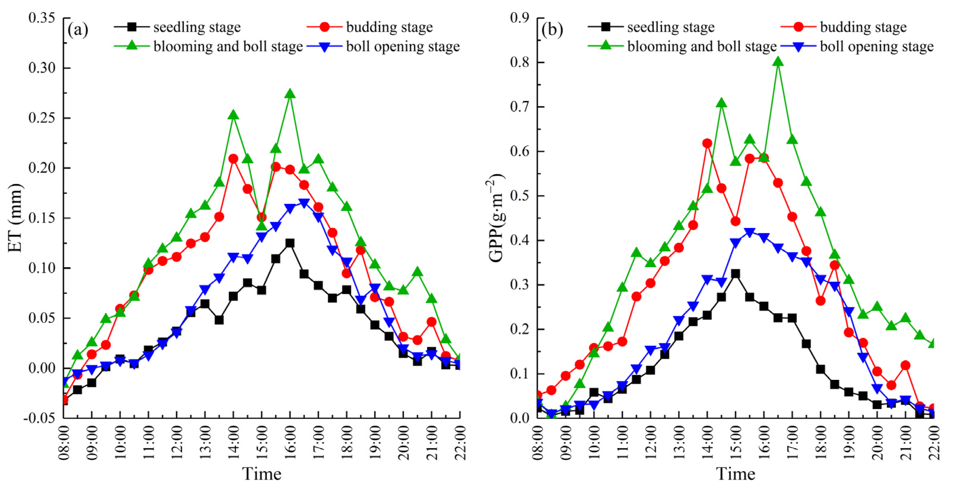
3.2. ET and GPP
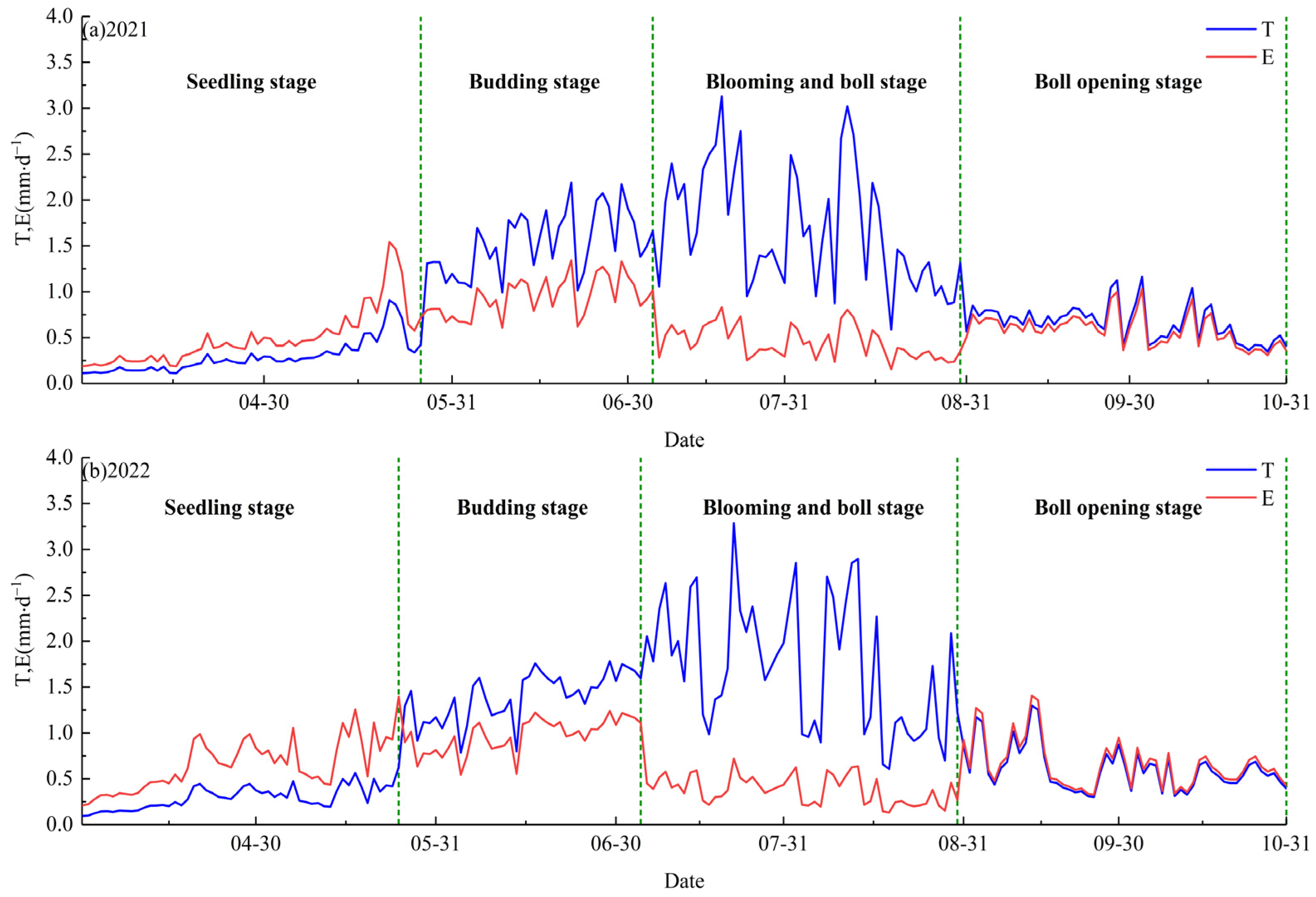
3.3. ET Components
4. Discussion
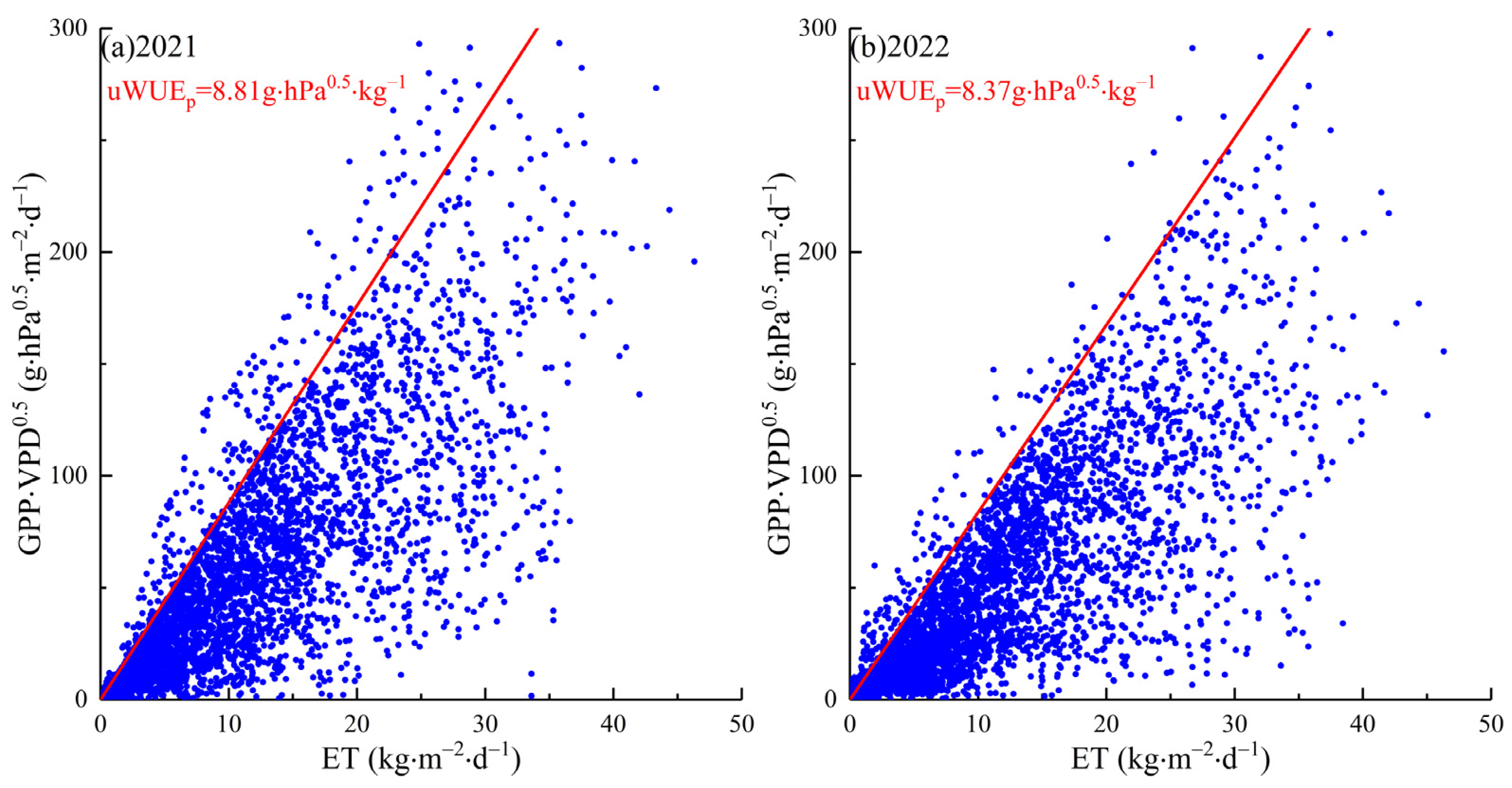
4.1. uWUE Influencing Factors
4.2. Causes of Changes in ET and GPP
4.3. Causes of Changes in T/ET
5. Conclusions
Author Contributions
Funding
Data Availability Statement
Acknowledgments
Conflicts of Interest
References
- Ma, N.; Zhang, Y.; Guo, Y.; Gao, H.; Zhang, H.; Wang, Y. Environmental and biophysical controls on the evapotranspiration over the highest alpine steppe. J. Hydrol. 2015, 529, 980–992. [Google Scholar] [CrossRef]
- Liu, B.; Cui, Y.; Luo, Y.; Shi, Y.; Liu, M.; Liu, F. Energy partitioning and evapotranspiration over a rotated paddy field in Southern China. Agric. For. Meteorol. 2019, 276–277, 107626. [Google Scholar] [CrossRef]
- Liu, X.; Wang, G.; Yang, S.; Xu, J.; Wang, Y. Influence Factors and Characteristics of Transpiration and Evaporation in Water-saving Irrigation Paddy Field under Different Temporal Scales. Trans. Chin. Soc. Agric. Mach. 2016, 47, 91–100+170. [Google Scholar]
- Stocker Thomas, F.; Raible Christoph, C. Climate change: Water cycle shifts gear. Nature 2005, 434, 830–833. [Google Scholar] [CrossRef] [PubMed]
- Feng, Y.; Gong, D.-Z.; Wang, H.-B.; Hao, W.-P.; Mei, X.-R.; Cui, N.-B. Estimating Rainfed Maize Evapotranspiration Using the FAO Dual Crop Coefficient Method on the Loess Plateau. Chin. J. Agrometeorol. 2017, 38, 141–149. [Google Scholar]
- Liu, X.-Y.; Li, Y.-Z.; Zhong, X.-L.; Cao, J.-F.; Yuan, X.-H. Evaluation of 16 Models for Reference Crop Evapotranspiration (ET0) Based on Daily Values of Weighing Lysimeter Measurements. Chin. J. Agrometeorol. 2017, 38, 278–291. [Google Scholar]
- Zhao, W.; Ji, X.; Liu, H. Progresses in Evapotranspiration Research and Prospect in Desert Oasis Evapotranspiration Research. Arid Zone Res. 2011, 28, 463–470. [Google Scholar]
- Wu, Y.; Du, T. Estimating and partitioning evapotranspiration of maize farmland based on stable oxygen isotope. Trans. Chin. Soc. Agric. Eng. (Trans. CSAE) 2020, 36, 127–134. [Google Scholar]
- Xu, X.W.; Yu, X.X.; Jia, G.D.; Li, H.Z.; Lu, W.W.; Liu, Z.Q. A review of water and carbon flux partitioning and coupling in SPAC using stable isotope techniques. Chin. J. Appl. Ecol. 2017, 28, 2369–2378. [Google Scholar]
- Wu, Y.; Du, T. Evaporation and its influencing factors in farmland soil in the arid region of Northwest China. Trans. Chin. Soc. Agric. Eng. (Trans. CSAE) 2020, 36, 110–116. [Google Scholar]
- Rafi, Z.; Merlin, O.; Le Dantec, V.; Khabba, S.; Mordelet, P.; Er-Raki, S.; Amazirh, A.; Olivera-Guerra, L.; Hssaine, B.A.; Simonneaux, V.; et al. Partitioning evapotranspiration of a drip-irrigated wheat crop: Inter-comparing eddy covariance-, sap flow-, lysimeter- and FAO-based methods. Agric. For. Meteorol. 2019, 265, 310–326. [Google Scholar] [CrossRef]
- Griffis, T.J. Tracing the flow of carbon dioxide and water vapor between the biosphere and atmosphere: A review of optical isotope techniques and their application. Agric. For. Meteorol. 2013, 174–175, 85–109. [Google Scholar] [CrossRef]
- Gu, L.; Meyers, T.; Pallardy, S.G.; Hanson, P.J.; Yang, B.; Heuer, M.; Hosman, K.P.; Liu, Q.; Riggs, J.S.; Sluss, D.; et al. Influences of biomass heat and biochemical energy storages on the land surface fluxes and radiative temperature. J. Geophys. Res. Atmos. 2007, 112, D02107. [Google Scholar]
- Zhou, S.; Yu, B.; Zhang, Y.; Huang, Y.; Wang, G. Water use efficiency and evapotranspiration partitioning for three typical ecosystems in the Heihe River Basin, northwestern China. Agric. For. Meteorol. 2018, 253–254, 261–273. [Google Scholar] [CrossRef]
- Wilson, K.B.; Hanson, P.J.; Mulholland, P.J.; Baldocchi, D.D.; Wullschleger, S.D. A comparison of methods for determining forest evapotranspiration and its components: Sap-flow, soil water budget, eddy covariance and catchment water balance. Agric. For. Meteorol. 2001, 106, 153–168. [Google Scholar] [CrossRef]
- Shuttleworth, W.J.; Wallace, J.S. Evaporation from sparse crops-an energy combination theory. Q. J. R. Meteorol. Soc. 1985, 111, 839–855. [Google Scholar] [CrossRef]
- Kool, D.; Agam, N.; Lazarovitch, N.; Heitman, J.L.; Sauer, T.J.; Ben-Gal, A. A review of approaches for evapotranspiration partitioning. Agric. For. Meteorol. 2014, 184, 56–70. [Google Scholar] [CrossRef]
- Zhou, S.; Yu, B.; Huang, Y.; Wang, G. The effect of vapor pressure deficit on water use efficiency at the subdaily time scale. Geophys. Res. Lett. 2014, 41, 5005–5013. [Google Scholar] [CrossRef]
- Zhou, S.; Yu, B.; Huang, Y.; Wang, G. Daily underlying water use efficiency for AmeriFlux sites. J. Geophys. Res. Biogeosci. 2015, 120, 887–902. [Google Scholar] [CrossRef]
- Zhou, S.; Yu, B.; Zhang, Y.; Huang, Y.; Wang, G. Partitioning evapotranspiration based on the concept of underlying water use efficiency. Water Resour. Res. 2016, 52, 1160–1175. [Google Scholar] [CrossRef]
- Berkelhammer, M.; Noone, D.C.; Wong, T.E.; Burns, S.P.; Knowles, J.F.; Kaushik, A.; Blanken, P.D.; Williams, M.W. Convergent approaches to determine an ecosystem’s transpiration fraction. Glob. Biogeochem. Cycles 2016, 30, 933–951. [Google Scholar] [CrossRef]
- Ning, Y. Water Use Efficiency and Its Response to T/ET of Maize Field in Longzhong Semi-Arid Area. Master’s Thesis, Lanzhou University, Lanzhou, China, 2018. [Google Scholar]
- Ma, S.; Eichelmann, E.; Wolf, S.; Rey-Sanchez, C.; Baldocchi, D.D. Transpiration and evaporation in a Californian oak-grass savanna: Field measurements and partitioning model results. Agric. For. Meteorol. 2020, 295, 108–204. [Google Scholar] [CrossRef]
- Liu, B.; Wang, W.; Cui, Y.; Xu, T. Partitioning evapotranspiration using the water-carbon flux coupling in a paddy field in the Middle and Lower Reaches of the Yangtze River in China. Trans. Chin. Soc. Agric. Eng. (Trans. CSAE) 2021, 37, 94–101. [Google Scholar]
- Cao, R.; Huang, H.; Wu, G.; Han, D.; Jiang, Z.; Di, K.; Hu, Z. Spatiotemporal variations in the ratio of transpiration to evapotranspiration and its controlling factors across terrestrial biomes. Agric. For. Meteorol. 2022, 321, 108984. [Google Scholar] [CrossRef]
- Da, R.A.E.Q.; Alvarez, S.E.; Andres, P. Partitioning evapotranspiration in a tallgrass prairie using micrometeorological and water use efficiency approaches under contrasting rainfall regimes. J. Hydrol. 2022, 608, 127624. [Google Scholar]
- GB/T 50485-2020; National Standard of the People’s Republic of China: Technical Standard for Microirrigation Engineering. China Planning Press: Beijing, China, 2020.
- SL 13-2015; Standard of Ministry of Water Resources of the People’s Republic of China: Specifications for Irrigation Experiment. China Water & Power Press: Beijing, China, 2015.
- Burba, G. The Eddy Covariance Method; LI-COR Biosciences: Lincoln, NE, USA, 2013; p. 331. [Google Scholar]
- Webb, E.K.; Pearman, G.; Leuning, R. Correction of flux measurements for density effects due to heat and water vapour transfer. Q. J. R. Meteorol. Soc. 1980, 106, 85–100. [Google Scholar] [CrossRef]
- Lee, X.; Massman, W.J. A Perspective on Thirty Years of the Webb, Pearman and Leuning Density Corrections. Bound.-Layer Meteorol. 2011, 139, 37–59. [Google Scholar] [CrossRef]
- Mauder, M.; Foken, T. Impact of post-field data processing on eddy covariance flux estimates and energy balance closure. Meteorol. Z. 2006, 15, 597–609. [Google Scholar] [CrossRef]
- Hobbs, S. Atmospheric boundary layer flows: Their structure and measurement. J. Atmos. Terr. Phys. 1995, 57, 1357. [Google Scholar] [CrossRef]
- Wilczak, J.M.; Oncley, S.P.; Stage, S.A. Sonic Anemometer Tilt Correction Algorithms. Bound.-Layer Meteorol. 2001, 99, 127–150. [Google Scholar] [CrossRef]
- Wei, J.; Xu, H.; Zhou, L.; Cheng, X.; Tang, X.; Fu, Z.; Tang, Q.; Tang, J. Seasonal variation in carbon exchange and its modulating factors of a double cropping rice ecosystem in Southern China. J. Agro-Environ. Sci. 2018, 37, 1035–1044. [Google Scholar]
- Zhu, Z.; Sun, X.; Zhou, Y.; Xu, J.; Yuan, G. Correction method for eddy covariance fluxes of non-flat underlying surface and its application in ChinaFLUX. Sci. China Ser. D Earth Sci. 2004, S2, 37–45. [Google Scholar]
- Xing, Q.; Han, G.; Yu, J.B.; Wu, L.X.; Yang, L.; Mao, P.L.; Wang, G.; Xie, B. Net ecosystem CO2 exchange and its controlling factors during the growing season in an inter-tidal salt marsh in the Yellow River Estuary. Acta Ecol. Sin. 2014, 34, 4966–4979. [Google Scholar]
- Baldocchi, D.D. Assessing ecosystem carbon balance: Problems and prospects of the eddy covariance technique. Glob. Chang. Biol. 2003, 9, 478–492. [Google Scholar] [CrossRef]
- Falge, E.; Baldocchi, D.; Olson, R.; Anthoni, P.; Aubinet, M.; Bernhofer, C.; Burba, G.; Ceulemans, R.; Clement, R.; Dolman, H.; et al. Gap filling strategies for defensible annual sums of net ecosystem exchange. Agric. For. Meteorol. 2001, 107, 43–69. [Google Scholar] [CrossRef]
- Lloyd, J.; Taylor, J.A. On the Temperature Dependence of Soil Respiration. Funct. Ecol. 1994, 8, 315–323. [Google Scholar] [CrossRef]
- Guo, W.H.; Kang, S.Z.; Li, F.S.; Li, S.E. Variation of NEE and its affecting factors in a vineyard of arid region of northwest China. Atmos. Environ. 2014, 84, 349–354. [Google Scholar] [CrossRef]
- Gilmanov, T.G.; Verma, S.B.; Sims, P.L.; Meyers, T.P.; Bradford, J.A.; Burba, G.G.; Suyker, A.E. Gross primary production and light response parameters of four Southern Plains ecosystems estimated using long-term CO2-flux tower measurements. Glob. Biogeochem. Cycles 2003, 17, 1071. [Google Scholar] [CrossRef]
- Cade, B.S.; Noon, B.R. A Gentle Introduction to Quantile Regression for Ecologists. Front. Ecol. Environ. 2003, 1, 412–420. [Google Scholar] [CrossRef]
- Yu, K.; Moyeed, R.A. Bayesian quantile regression. Stat. Probab. Lett. 2001, 54, 437–447. [Google Scholar] [CrossRef]
- Bremnes, J.B. Probabilistic wind power forecasts using local quantile regression. Wind Energy 2004, 7, 47–54. [Google Scholar] [CrossRef]
- Wang, L.; Good, S.P.; Caylor, K.K. Global synthesis of vegetation control on evapotranspiration partitioning. Geophys. Res. Lett. 2014, 41, 6753–6757. [Google Scholar] [CrossRef]
- Wang, X.F.; Hu, S.J.; Tian, C.Y.; Luo, Y. The changing law of the diurnal evapotranspiration and soil evaporation in cotton field of Tarim irrigation area. Agric. Res. Arid. Areas 2012, 30, 74–78. [Google Scholar]


| Year | uWUEa/g·hpa0.5·kg−1 | uWUEp/g·hpa0.5·kg−1 | |||
|---|---|---|---|---|---|
| Seedling Stage | Budding Stage | Blooming and Boll Stage | Boll Opening Stage | The Whole Stage | |
| 2021 | 3.26 | 5.46 | 6.96 | 4.67 | 8.81 |
| 2022 | 2.59 | 4.94 | 6.86 | 4.02 | 8.37 |
| Year | Component | Seedling Stage | Budding Stage | Blooming and Boll Stage | Boll Opening Stage | The Whole Stage |
|---|---|---|---|---|---|---|
| 2021 | ET/mm | 47.31 | 87.94 | 104.32 | 64.78 | 304.34 |
| T/ET | 0.37 | 0.62 | 0.79 | 0.53 | 0.62 | |
| T/mm | 17.50 | 54.52 | 82.41 | 34.33 | 188.77 | |
| E/mm | 29.80 | 33.42 | 21.91 | 30.45 | 115.57 | |
| 2022 | ET/mm | 49.93 | 92.356 | 107.91 | 67.27 | 317.46 |
| T/ET | 0.31 | 0.59 | 0.82 | 0.48 | 0.60 | |
| T/mm | 15.48 | 54.49 | 88.48 | 32.29 | 190.74 | |
| E/mm | 34.45 | 37.87 | 19.42 | 34.98 | 126.72 |
| Growth Stage | Component | Tair | RH | Rn | VPD |
|---|---|---|---|---|---|
| Seedling stage | T | 0.54 | −0.29 | 0.58 | 0.21 |
| E | 0.53 | −0.27 | 0.58 | 0.21 | |
| ET | 0.53 | −0.28 | 0.58 | 0.21 | |
| Budding stage | T | 0.61 | −0.32 | 0.60 | −0.18 |
| E | 0.63 | −0.32 | 0.63 | −0.22 | |
| ET | 0.63 | −0.32 | 0.62 | −0.20 | |
| Blooming and boll stage | T | 0.63 | −0.45 | 0.49 | −0.16 |
| E | 0.56 | −0.39 | 0.43 | −0.19 | |
| ET | 0.62 | −0.44 | 0.48 | −0.17 | |
| Boll opening stage | T | 0.50 | −0.21 | 0.65 | 0.54 |
| E | 0.48 | −0.20 | 0.63 | 0.53 | |
| ET | 0.49 | −0.21 | 0.64 | 0.54 | |
| The whole stage | T | 0.73 | −0.02 | 0.59 | 0.27 |
| E | 0.24 | −0.07 | 0.25 | 0.18 | |
| ET | 0.71 | −0.08 | 0.59 | 0.30 |
Disclaimer/Publisher’s Note: The statements, opinions and data contained in all publications are solely those of the individual author(s) and contributor(s) and not of MDPI and/or the editor(s). MDPI and/or the editor(s) disclaim responsibility for any injury to people or property resulting from any ideas, methods, instructions or products referred to in the content. |
© 2023 by the authors. Licensee MDPI, Basel, Switzerland. This article is an open access article distributed under the terms and conditions of the Creative Commons Attribution (CC BY) license (https://creativecommons.org/licenses/by/4.0/).
Share and Cite
Liu, Y.; Qiao, C. Partitioning Evapotranspiration in a Cotton Field under Mulched Drip Irrigation Based on the Water-Carbon Fluxes Coupling in an Arid Region in Northwestern China. Agriculture 2023, 13, 1219. https://doi.org/10.3390/agriculture13061219
Liu Y, Qiao C. Partitioning Evapotranspiration in a Cotton Field under Mulched Drip Irrigation Based on the Water-Carbon Fluxes Coupling in an Arid Region in Northwestern China. Agriculture. 2023; 13(6):1219. https://doi.org/10.3390/agriculture13061219
Chicago/Turabian StyleLiu, Yanxue, and Changlu Qiao. 2023. "Partitioning Evapotranspiration in a Cotton Field under Mulched Drip Irrigation Based on the Water-Carbon Fluxes Coupling in an Arid Region in Northwestern China" Agriculture 13, no. 6: 1219. https://doi.org/10.3390/agriculture13061219
APA StyleLiu, Y., & Qiao, C. (2023). Partitioning Evapotranspiration in a Cotton Field under Mulched Drip Irrigation Based on the Water-Carbon Fluxes Coupling in an Arid Region in Northwestern China. Agriculture, 13(6), 1219. https://doi.org/10.3390/agriculture13061219