Analysis of the Spatio-Temporal Evolution, Influencing Factors, and Spillover Effects of the Urban–Rural Income Gap in Chongqing Municipality, China

Abstract

In addition to being necessary for the stability, coordination, and sustainable growth of the national economy, narrowing the urban–rural income gap is also an “Important national matter” for the long-term security of the nation. “Big mountain areas, big cities, big reservoir areas, big rural areas, and ethnic areas” are all present in the municipality of Chongqing. All of the poverty-stricken counties have been lifted out of poverty, despite the promotion of targeted poverty alleviation and other policies, significant urban–rural income gaps remain. In view of the current research, there has been no in-depth discussion on the correlation between urban and rural income gap and poverty levels in various regions, and there has been no in-depth discussion on the spatial correlation and spillover effects of various influencing factors. This paper employs panel data from 2010 to 2021 for 37 counties in Chongqing; based on an analysis of the characteristics of the urban–rural income gap’s spatial pattern and spatio-temporal evolution, it classifies each county (city and district) as either a non-poverty or poverty-stricken county and uses spatial econometric models to conduct an in-depth study of the influencing factors and spillover effects of the urban–rural income gap in Chongqing. The outcomes of our analysis of the influencing factors reveal that the level of fixed assets investment, the per capita spending of public funds, the proportion of rural employees, the proportion of grain sowing, the amount of agricultural fertilizer applied per unit area, the proportion of real estate development investment, and population density variables are important causes of the URIG in Chongqing. The spillover effects of these factors vary between poverty-stricken and non-poverty-stricken counties. This paper aims to provide reference to policymakers to design measures to narrow the urban–rural income gap and advance the urban–rural coordinated development strategy on the basis of a thorough examination of the spatial and temporal evolution, influencing variables, and spillover effects of the urban–rural income gap in Chongqing.

1. Introduction

Narrowing the income gap, to a large extent, means narrowing the wealth gap, which is an “Important national matter,” related to the long-term stability of the nation and is necessary for the stable, coordinated, and sustainable growth of the national economy [1]. China’s economy has experienced remarkable growth over the past 40 years, and its citizens’ living standards and per capita disposable income have both dramatically improved [2]. However, the growth of the “cake” of total income has caused the problem of a widening income gap [3]. The issue of the income gap is progressively becoming a major barrier to China’s development into an all-around prosperous society and even a modern nation. One of the key forms of the income gap is the urban–rural income gap (URIG) [4]. The URIG accounts for between 30% and 50% of China’s income gap, according to Sicular et al. (2007) [5]. It is clear that the income gap’s primary manifestation is the URIG.

China’s URIG is generally high and has been trending upward for a considerable amount of time [6]. The URIG in China has shown a tendency to increase, and then decrease since 2000, peaking at 3.11 in 2009, and it has been reducing slowly for more than 10 years. By 2020, the ratio had shrunk to 2.56 [7]. Being supported by a number of strong preferences, China’s URIG has been reduced to some extent and has tended to narrow gradually in recent years. It is undeniable that China’s URIG is still greater than the global average [8]. Most notably, one study demonstrated that rural residents’ income level is strongly correlated with the URIG and typically exhibits an apparent reversal trend. That is, the URIG widens when rural residents’ income levels fall [9]. Premier Li Keqiang states that 600 million Chinese people earn CNY 1000 per month, which has raised concerns among the public [10]. Nowadays, raising rural incomes, narrowing the URIG, and realizing widespread prosperity have become vital issues to be solved in China’s modernization drive [11].

Located in the upper sections of the Yangtze River, Chongqing is the only municipality in central and western China that is directly under the control of the central government. As well as having the qualities of a large metropolis, it also combines large rural areas, mountains, reservoirs, and communities of ethnic minority residents. This paper chooses Chongqing as its representative research object. In China’s Chongqing municipality, the growth of the economy has been sluggish, and there are widespread cases of poverty. Urban and rural development have historically been uneven. There are 38 counties and districts within the municipality’s boundaries. This includes 18 poverty-stricken counties. Only five districts have no rural poverty alleviation task, of which Yuzhong District has almost no rural population. Although it has increasingly decreased, the URIG in Chongqing has been exceptionally slow to narrow over the last ten years. The urban–rural income ratio in Chongqing was still 2.45 in 2020, which is above the international warning line [12]; this significantly hinders urban and rural growth and revitalization. Promoting urban–rural integration and growth are crucial to the national rural revitalization strategy [13,14,15]. To address the problems and shortcomings of the existing literature, which fails to explore the correlation between the URIG and poverty levels in different regions, as well as the spatial correlation and spillover effects of various influencing factors, this study employs panel data from 2010 to 2021 for 37 counties in Chongqing (note: Yuzhong District is not included in the scope of this paper because there is no rural population). Using a study of the characteristics of the spatio-temporal evolution of the URIG, the counties (districts) are classified separately as non-poverty-stricken counties and poverty-stricken counties, and the spatial econometric model is used to study the influencing factors and spillover effects of URIG in Chongqing. This study aims to provide a theoretical basis and practical guidance for policymakers to rationally formulate measures to narrow the URIG and encourage urban–rural integration.

2. Literature Review

The issue of the URIG has gradually attracted the academic community’s attention [16]. Petty identified the industrial income gap as an issue, and Clark went into more detail as to the reasons why the URIG exists [17]. The causes of the URIG were examined by David Ricardo [18]. According to Kuznets (1955), as the economy grows, the URIG will first widen, and then narrow [19]. In other words, a developing country must experience an increasing URIG, but with the economy’s continued growth, the gap will progressively narrow after reaching a peak. The Kuznets (1955) hypothesis has been supported and confirmed by most people [20,21,22], but some scholars believe that this theory is unreliable. They suggest that there might only be a one-way relationship, or a random walk process, between economic growth and the URIG [23,24,25,26,27,28]. Despite it being the world’s largest developing nation, China’s general URIG has remained substantial in recent years. Although the URIG has reduced as a result of the implementation of precise poverty alleviation programs, the change has not been fundamental; the issue of China’s significant URIG still exists and will continue to do so for many years to come [9,29]. Evolving trends and influencing elements of the URIG have not been thoroughly explored in many previous research works. According to an overview of the literature, the following categories best describe the extant research. First, there are studies of the impact of economic growth [30,31,32,33,34], fiscal reform [35], rural financial development [36], targeted poverty alleviation (TPA) policy [1,2,4,37,38], labor migration [39,40], industrial development [41], and other independent variables influencing the URIG. Although this type of research is innovative, this kind of research focuses on the effects of a single factor on the URIG; it remains necessary to adequately examine and summarize the fundamental causes of the substantial URIG. The second type analyzes the URIG’s spatio-temporal evolution, and then discusses its regularity [42,43,44,45,46]. This kind of research has reference value because it can give policymakers an intuitive understanding of the URIG in the region in advance. Nevertheless, this kind of research only analyzes the spatial-temporal evolution characteristics of URIG, and more discussions of its formation are required. The third kind explores the elements that affect the URIG from various angles [47,48,49,50,51,52,53]. Compared with the other categories, these studies can more clearly show the factors that influence the URIG. However, most current studies neglect the spatial link between nearby study regions. Furthermore, although certain factors may affect the URIG in a given location, according to the first rule of geography, this impact may spread to nearby places, indirectly impacting the URIG and having positive or negative spillover effects.

After summarizing the existing research, we found that, despite its many achievements, there are still some deficiencies in studies of the factors driving the URIG. For instance, most studies solely examine the URIG itself, neglecting to examine its relationships with regional poverty, the national TPA policy, the rural regeneration strategy, and urban–rural integration. In addition, a thorough examination and discussion of the space–time evolution, influencing variables, and spillover effects of the urban–rural income difference are also frequently lacking in existing studies. Most critically, a crucial issue has been disregarded by previous studies: a region’s economic progress or level of poverty is likely to be correlated with the extent of the URIG in that region. Simply discussing the URIG as a whole is not conducive to elucidating the differences between influencing factors within the regions with different economic development levels. Discussing the spatio-temporal, influencing, and spillover effects will enable us to better understand the URIG and its causes. It will also help policymakers develop URIG-reducing countermeasures and shared prosperity strategies.

3. Materials and Methods

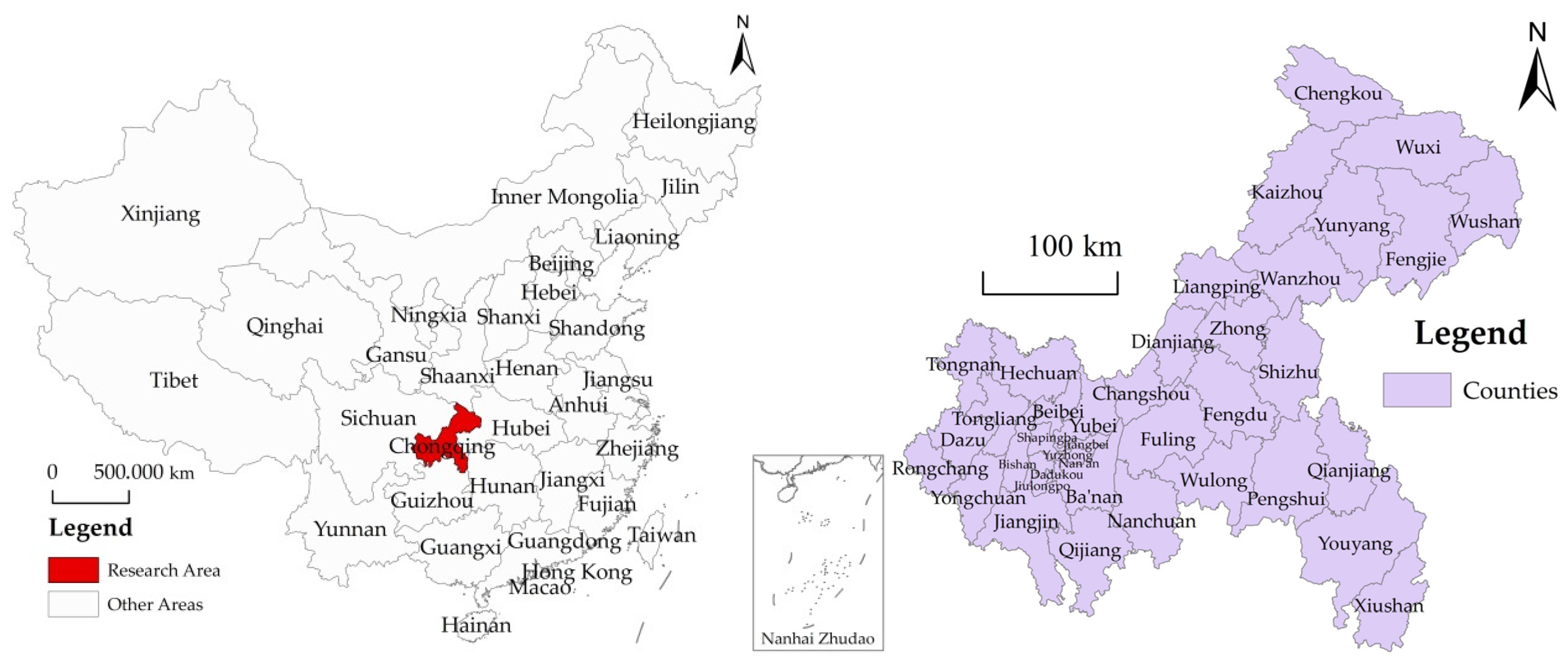
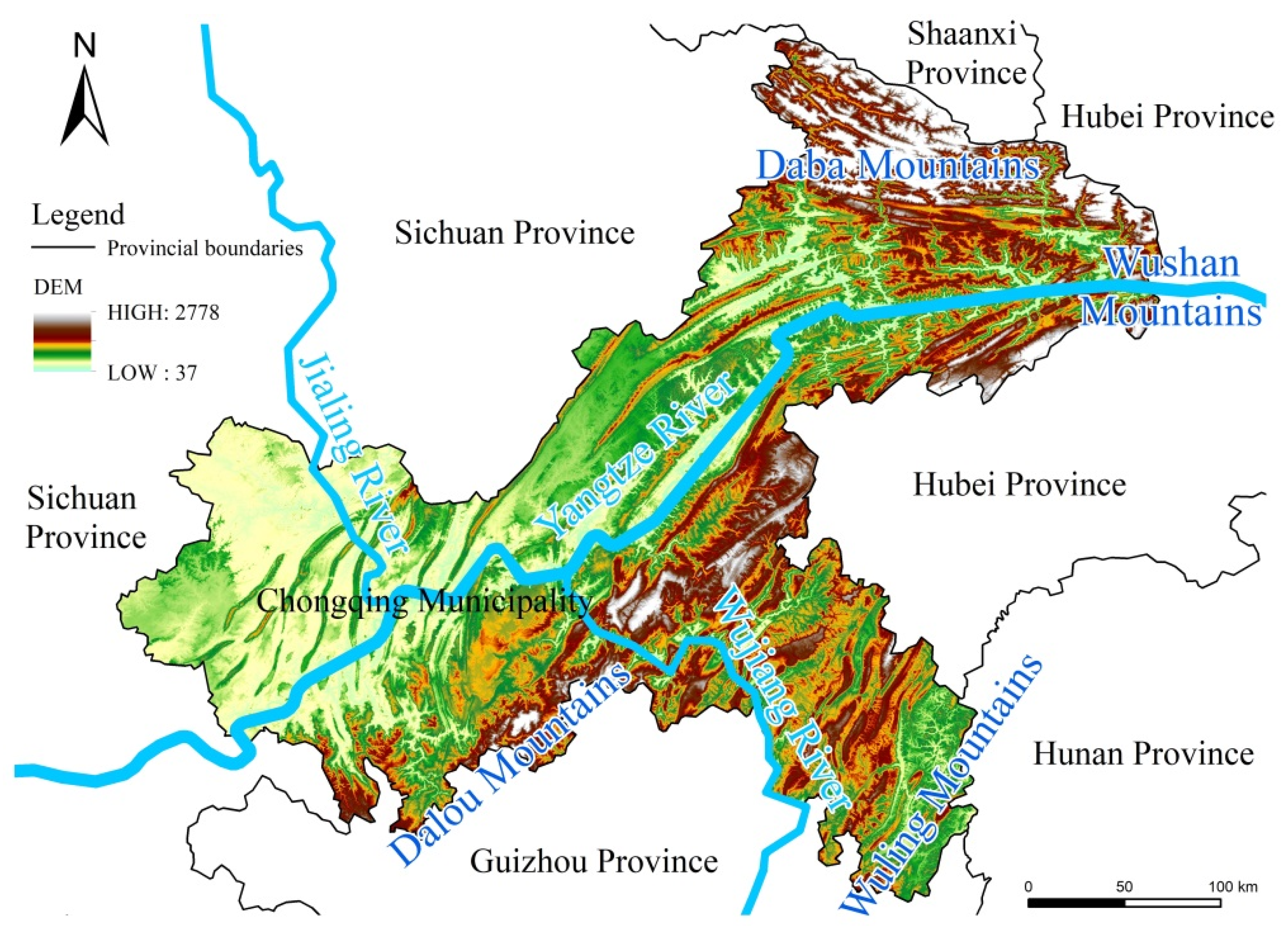
3.1. Overview of the Study Area

South-west China’s Chongqing Municipality, which is located along the upper Yangtze River, is situated between latitudes 105°11′ and 110°11′ east and 28°10′ and 32°13′ north. The Yangtze River’s main channel traverses the entire region from west to east over a distance of 665 km, cutting through three anticlines of Wushan Mountain to create the renowned Qutang Gorge, Wuxia Gorge, and Xiling Gorge (located in Hubei Province), i.e., the Yangtze River’s Three Gorges, which are renowned worldwide (Figure 1). In central and western China, Chongqing is a municipality, including “big cities, big villages, big mountain areas, large reservoir areas and ethnic minority areas”. The presence of a big city means that it is one of China’s four municipalities and the only municipality in the central and western regions. It is “big” insofar as it has a large geographical range: 82,400 square kilometers of land, or 2.4 times the total area of Beijing, Tianjin, and Shanghai. Moreover, both the urban area and the built-up area sizes exceed those of Shanghai and Tianjin [7] (China Statistical Yearbook). Additionally, the total population and urban population are larger than those of Beijing, Tianjin, and Shanghai. Regarding big rural areas, there are a wide range of rural areas in Chongqing, accounting for 95% of the whole city, and there is a sizable rural population. By the end of 2021, 9.53 million rural people—or approximately 1.3 times the combined rural populations of Beijing, Tianjin, and Shanghai—made up 29.67% of Chongqing’s total population [7]. There are also many agriculture-related towns and villages. In total, 940 towns (streets) in Chongqing, or 91.2% of all the towns (streets), are tied to agriculture. There are 9048 rural cooperatives, which make up 80.6% of all the villages. The big mountain area refers to Chongqing, which has been known as a “mountain city” since ancient times. Its land forms are mainly hills and mountains, of which mountains account for about 76% [54]. The elevation varies greatly and the slope area is large (Figure 2). Chongqing’s Three Gorges Project Reservoir is the largest in China. There are 20 counties (cities) involved in the resettlement task, 16 of which are located in Chongqing. One of the reasons why the state established Chongqing as a municipality in March 1997 was to solve the problem of the relocation and resettlement of more than 1 million immigrants. Ethnic minority areas refer to cities where a certain number of ethnic minority residents are distributed. Chongqing has 2.1708 million ethnic minority residents, or 6.77% of the total population, according to the Primary Statistics of the Seventh National Population Census [55]; foremost among them are Tujia and Miao people, who are concentrated in the south-east of the city. Four ethnically autonomous counties exist (Shizhu, Xiushan, Youyan, and Pengshui). Because Chongqing is a municipality and has the characteristics of a large developed city, but also has the characteristics of a large rural area characterized by large mountains, reservoirs, and ethnic minority areas, urban and rural development within the city is very uneven. There are 38 counties and districts within the municipality’s boundaries. These include 18 poverty-stricken counties. There are 18 deeply poverty-stricken towns at the municipal level, 1919 impoverished villages, and 1.659 million poor people. At the end of 2020, even with the success of the national poverty alleviation program, there were still 4 national key counties for rural revitalization and 17 municipal key towns for rural revitalization. In 2020, Chongqing’s urban per capita disposable income (PCDI) was CNY 40006, making it rank 13th among China’s 31 provinces (autonomous areas, municipalities). The rural residents’ PCDI is CNY 16361, placing them in 15th out of the country’s 31 provinces (autonomous areas, municipalities). In all counties (districts) in the municipality, there is a large gap in PCDI between urban and rural residents. In 2020, CNY 46,994 was the greatest PCDI for urban residents (Yuzhong District), and the lowest one was CNY 28,357 (Wuxi County); CNY 24,869 was the greatest PCDI for rural residents (Nan’an District), and the lowest one was CNY 11,123 (Wuxi County) [56].

3.2. Research Methods of Spatial Econometrics

Spatial econometrics is used widely. Because of its ability to deal with spatial autocorrelation, spatial econometrics has increasingly become a cutting-edge and mainstream discipline [57]. This paper focuses on 37 counties in Chongqing (Yuzhong District has almost no rural population, so it is not within the scope of this study), and so, data analysis issues with spatial autocorrelation might be more evident. Consequently, it is appropriate to evaluate the contributing causes and spillover effects of the URIG using the spatial econometrics method. It is vital to choose the right spatial weight matrix before creating the model. Neighboring spatial weight matrices and spatial inverse distance matrices are frequently employed. Within the spatial adjacency matrix, the adjacency between two places is 1; otherwise, it is 0. Therefore, this matrix has an obvious drawback: it ignores the correlation differences between adjacent areas. The spatial inverse distance weight matrix can improve this problem; nonetheless, this matrix disregards the relationship between distant regions. That is to say, although two regions may not be close to each other, the closer regions generally have more obvious spatial correlation than those that are further apart do. Considering this, this research improves the two matrices described above. By using the reciprocal of the linear distance between the two centers as the weight, it builds an enhanced spatial inverse distance weight matrix. The weight increases as the linear distance between two points decreases, meaning that it can better avoid the problem of the “rough” setting of the above two weight matrices. The model estimation results also further indicate that the geographic autocorrelation issue of the URIG in Chongqing can be more effectively resolved by the improved spatial inverse distance weight matrix. Based on this, this paper intends to select an appropriate weight matrix, and then use spatial econometric models to analyze its influencing factors, aiming to better control the spatial autocorrelation problem and accurately obtain estimated results. At the same time, this paper intends to use this method to further explore the spatial spillover effects of core influencing factors.

After setting the weight matrix, it is necessary to calculate its spatial autocorrelation degree. Moran’s I can provide a sufficient answer to the question of spatial correlation between regions. The following formula is the Moran’s I calculation [58]:

$$\mathrm{Moran}’\mathrm{s} \mathrm{I}=\frac{n{\mathit{e}}^{\mathrm{T}}\mathit{W}\mathit{e}}{{\mathit{e}}^{\mathrm{T}}\mathit{e}\left({\displaystyle {\sum }_i{\displaystyle {\sum }_j{w}_{ij}}}\right)}=\frac{{\displaystyle {\sum }_i{\displaystyle {\sum }_j{w}_{ij}(x_i-\overline{x}\left)\right(y_i-\overline{y})}}}{S^2\left({\displaystyle {\sum }_i{\displaystyle {\sum }_j{w}_{ij}}}\right)}$$

(1)

where the residual matrix is denoted by e; the spatial weight matrix is abbreviated to W; the observed value x variance is represented by S².

For data with spatial autocorrelation, the use of traditional estimation methods cannot control the spatial correlation well, and it is easy to bring a bias to the model regression. Hence, the spatial econometric method is more capable of accurate estimation. It is possible to express the generalized spatial panel model as [57]:

$$\{\begin{array}{c}{Y}_{it}=\tau Y_{i,t-1}+\rho {\mathit{W}}_i{\mathit{Y}}_t+{\mathit{X}}_{it}\mathbf{\beta }+{\mathit{D}}_i\mathit{X}\mathbf{\delta }+u_i+{\gamma }_t+{\epsilon }_{it}\\ {\epsilon }_{it}=\lambda {\mathit{M}}_i{\epsilon }_t+v_{it}\end{array}$$

(2)

where the explained Y_it variable’s first-order lag term is represented by Y_i,t−1 (i.e., τ ≠ 0 is the spatial dynamic panel model); the ith row of the spatial weight matrix W, D, and M is represented by W_i, D_i, and M_i. The ith line of the explanatory variable matrix is represented by X_it. The parameter vector to estimate is β. δ stands for an unknown and fixed parameter vector that needs to be approximated; the fixed effect is referred to as u_i. γ_t represents the time effect, and ε_it stands for the residual.

The above model is too general and can be transformed under specific conditions. For general panels, the Spatial Autoregressive Model with Spatial Autoregressive Districts (SARAR), Spatial Durbin Model (SDM), Spatial Error Model (SEM), and Spatial Autoregressive Model (SAR) can be used [59].

Not only can the spatial econometric model accurately estimate the regression parameters with spatial autocorrelation data, but it can also conveniently analyze the spillover effect of an impact factor regarding the surrounding area. Accordingly, in order to provide guidance for narrowing the URIG and achieving the goal of shared prosperity, the author of this study use the spatial econometric model to explore the various factors that influence the URIG in Chongqing and their spillover effects on the surrounding areas.

3.3. Indicator System

Using knowledge from earlier studies [43,44,45,46,47,48,49] and taking into account the principles of data availability and representativeness, this study used the 2010–2021 PCDI ratio of urban and rural people in 37 Chongqing counties (cities and districts) to compute the URIG. The survey yearbook for Chongqing in 2022 served as the data source. It should be noted that China’s statistics on rural income are inconclusive. The per capita net income of rural residents served as the unifying concept until 2014; however, after that year, it was updated to reflect rural residents’ PCDI. However, from 2010 to 2014, information on the per capita disposable income of rural people in all of Chongqing’s counties was nevertheless published in the 2022 survey yearbook. Hence, the statistical caliber is consistent before and after, which is convenient for model analysis. At the same time, referring to the previous research results [43,44,45,46,47,48,49], this study collected panel data of 37 counties (cities and districts) in Chongqing from 2010 to 2021, including 7 dimensions of industrial structure, economic and social aspects, investment expenditure, rural development, agriculture status, urban construction, and population structure, as explanatory variables. See

Table 1. Index system and calculation method of the influencing factors.

Dimension	Variables	Computing Method	Name	Unit
Industrial Structure	Development level of primary industry	ln (primary industry output value/rural registered residence population)	X1	CNY/person
	Development level of secondary industry	ln (output value of secondary industry/urban registered residence population)	X2	CNY/person
	Development level of tertiary industry	ln (output value of tertiary industry/total population)	X3	CNY/person
	Development level of agriculture, forestry, animal husbandry, and fisheries	ln (total output value of agriculture, forestry, animal husbandry and fisheries/rural registered residence population)	X4	CNY/person
	Proportion of the output value of secondary and tertiary industries	Secondary and tertiary industries’ output value/GDP × 100%	X5	%
Economic and Social	Night light brightness	ln (night light + 0.01)	X6	None
	Economic development level	ln (GDP/total population)	X7	CNY/person
	Per capita grain output	ln (total grain output/total population)	X8	kg/person
Investment Expenditure	Fixed assets investment level	ln (total fixed assets investment/total population)	X9	CNY/person
	Per capita public financial expenditure	ln (public finance expenditure/total population)	X10	CNY/person
Rural Development	Proportion of rural employees	Total number of rural employees/total population × 100%	X11	%
Agriculture Status	Proportion of grain sown	Grain planting area/farm plants planting area × 100%	X12	%
	Amount of agricultural fertilizer used per unit area	ln (amount of agricultural fertilizer used/planting area of farm plants)	X13	kg/m2
Urban Construction	Minimum living security ratio of urban residents	Minimum living security number of urban residents/urban registered residence population × 100%	X14	%
	Proportion of real estate development investment	Investment in real estate development/GDP × 100%	X15	%
Population Structure	Urbanization rate	Urban registered residence population/total population × 100%	X16	%
	Population density	ln (total population/land area)	X17	person/km2

for specific indicators.

Table 1 lists the calculation methods, units, and variable names of various indicators in detail. The data source of night light is DMSP/OLS, which was processed using ArcGIS software. The data sources of all other indicators are the Chongqing Statistical Yearbook (2011–2022) and the EPS global statistical data/analysis platform.

4. Results

4.1. Analysis of the Spatial Pattern of the Urban–Rural Income Gap

It is essential to understand the spatio-temporal evolution pattern of the URIG in each county in Chongqing before analyzing the causes that influence the URIG in each county. The reason for this is that only through a thorough examination of the spatial-temporal change trends of the urban–rural income ratio in each county of Chongqing can we gain a more accurate understanding of the current state of the URIG in these areas, which serves as a guide for the examination of its influencing factors. Therefore, the paper collected the URIG of the 37 counties of Chongqing and the rural residents’ PCDI (Yuzhong District has no data, so it is not included) from 2010 to 2021. It then calculated the annual average value to obtain the annual average distribution of the PCDI of rural residents (Figure 3a) and the annual average distribution of the urban–rural income ratio in 37 counties in Chongqing (Figure 3b).

Figure 3 shows that the URIG in Chongqing is closely linked to the rural residents’ PCDI. Most counties in the west of Chongqing constitute non-poverty-stricken counties (Figure 3c), most of which are economically developed. Rural residents in these areas have a significantly higher PCDI than those in other areas do (Figure 3a). The urban–rural income ratio in these regions remains low (Figure 3b). At the same time, most counties in the central and eastern parts of Chongqing constitute poverty-stricken counties (Figure 3c). Most of them are economically underdeveloped zones, particularly those in Chongqing’s remote south-eastern and north-eastern areas. The PCDI of rural residents in these areas is notably lower than those in the rest of the districts (Figure 3a), and the urban–rural residents’ income ratio remains high. Chongqing’s URIG and rural PCDI are linked. Areas in Chongqing with a low URIG are generally non-poverty-stricken counties, as shown in Figure 3. In these areas, rural residents’ PCDI is typically higher. By comparison, areas with a higher URIG tend to be poverty-stricken counties, and rural residents’ PCDI in these regions is typically lower. There is a clear pattern of negative correlation between the URIG and the PCDI of rural residents. This is because the URIG calculated in this paper is the ratio of the PCDI of urban residents to the PCDI of rural residents. Based on the assumption that the PCDI of urban residents remains unchanged, as rural residents’ PCDI increases, the URIG decreases. Similarly, on the basis that the rural residents’ PCDI remains intact, as the PCDI of urban residents increases, the URIG increases. Nonetheless, our study found that urban residents in poverty-stricken counties have a lower PCDI than those in non-poverty-stricken counties do. Quite the opposite is true; the rural residents’ PCDI shows very obvious spatial differences, and this difference is significantly greater than the difference in PCDI of urban residents, which results in a higher URIG in places where the PCDI of rural residents is lower. Rural poverty is the main cause of the expansion of the URIG. The point of reducing the URIG is to improve rural residents’ income level. Only when the rural residents’ income level is significantly improved will the URIG in this region be significantly decreased.

From the perspective of spatial distribution, the above analysis mainly discusses the space distribution law of the URIG, but it remains to be determined whether there is an obvious spatial law of the URIG, and statistical data should be used for more accurate calculations (Appendix A:

Table A1. Calculation results of Moran’s I and Geary’s C from 2010 to 2021.

Year	Moran’s I	Z Statistics	p Values	Geary’s C	Z Statistics	p Values
2010	0.336 ***	12.996	0.000	0.642 ***	−10.582	0.000
2011	0.327 ***	12.649	0.000	0.637 ***	−10.803	0.000
2012	0.326 ***	12.620	0.000	0.639 ***	−10.649	0.000
2013	0.325 ***	12.573	0.000	0.639 ***	−10.738	0.000
2014	0.325 ***	12.580	0.000	0.640 ***	−10.730	0.000
2015	0.325 ***	12.597	0.000	0.640 ***	−10.712	0.000
2016	0.326 ***	12.624	0.000	0.636 ***	−10.869	0.000
2017	0.326 ***	12.626	0.000	0.635 ***	−10.921	0.000
2018	0.321 ***	12.444	0.000	0.640 ***	−10.687	0.000
2019	0.312 ***	12.148	0.000	0.645 ***	−10.397	0.000
2020	0.307 ***	11.981	0.000	0.648 ***	−10.285	0.000
2021	0.308 ***	12.012	0.000	0.647 ***	−10.338	0.000
Annual Average	0.324 ***	12.540	0.000	0.639 ***	−10.706	0.000

Note: *, **, and *** indicate the significance levels of 10%, 5%, and 1%, respectively.

).

Table A1 shows that both Moran’s I and Geary’s C passed the 1% significance test from 2010 to 2021 and for the average of each year, indicating that the urban–rural income ratio of Chongqing shows obvious spatial autocorrelation and positive agglomeration. For data with spatial autocorrelation, using the common model to study the influencing factors ignores the interference caused by spatial autocorrelation, resulting in deviation. Thus, this paper utilizes the spatial econometric model to study the influencing factors and spillover effects of the URIG in 37 counties of Chongqing in greater depth.

4.2. Analysis of the Spatio-Temporal Evolution of the Urban–Rural Income Gap

The above analysis examines the URIG’s spatial distributional pattern, and further explains its relationship with the rural residents’ income level and a county’s poverty level. However, the analysis can be further improved, as we cannot intuitively understand how big the difference is between poor and non-poverty-stricken counties. Accordingly, this paper intends to further explore the changing trends in the urban–rural income ratios of poor and non-poverty-stricken counties in Chongqing (Figure 4).

As shown in Figure 4, the URIG obviously differs between the two different types of counties, further supporting the above inference. In poverty-stricken counties, the average urban–rural income ratio reached 3.06 in 2010, and has shown a downward trend since then, falling to 2.42 in 2021, with a mean annual decline rate of decline of 2.13%. In 2010, non-poverty-stricken counties had an average urban-to-rural income ratio of 2.41, which is significantly lower than that of the poverty-stricken counties and has been showing a downward trend since then, falling to 1.97 in 2021, with a mean annual rate of decline of 1.85%. Overall, although the URIG is generally high in poverty-stricken counties, it has declined at a slightly higher rate than it has in non-poverty-stricken counties.

In general, the URIG in all of Chongqing’s counties has shown an annual drop, which may be related to poverty alleviation and rural construction. According to research conducted by Yang Renyi et al. (2022) [1,25], China’s TPA policy can significantly raise rural residents’ income level and decrease the URIG; so, China’s investment in and support for rural regions is the main cause of the URIG’s decrease. In addition, these authors also found evident differences in the level of the URIG between poverty-stricken and non-poverty-stricken counties in Chongqing. Therefore, it is necessary to discuss them separately when studying the influencing factors of URIG.

4.3. Analysis of the Influencing Factors of the Urban–Rural Income Gap

The above correlations indicate that the URIG in Chongqing has quite obvious spatial autocorrelation. Most areas in the west of Chongqing are low-value clusters, while those in the north-east and south-east are high-value clusters. The spatial econometric model is thus more appropriate for exploring its impact factors. Furthermore, the URIG in Chongqing is closely linked to a region’s level of poverty. Poverty-stricken counties typically have a greater URIG than non-poverty-stricken counties do. This significant difference indicates that the factors affecting the URIG in the two different types of counties in Chongqing may also differ, as may their effects. Therefore, it is particularly necessary to discuss them separately. Thus, in addition to analyzing the variables affecting the URIG in 37 counties of Chongqing, to assess the effects of the influencing elements of the URIG in various locations, this article will examine the influencing variables of the URIG in 19 counties of Chongqing that are not poor and 18 counties that are. The estimates of several models when the total sample was used are presented in

Table 2. Estimation results of the econometric model for the analysis of the influence factors of the urban–rural income gap.

Items	Influence Factors of the Urban–Rural Income Gap
	(1) FE	(2) SARAR	(3) SAR	(4) SEM
Development Level of Primary Industry (X1)	0.0001 (0.0075)	0.0011 (0.0031)	0.0011 (0.0031)	0.0010 (0.0031)
Development Level of Secondary Industry (X2)	0.0035 (0.0057)	0.0029 (0.0037)	0.0029 (0.0037)	0.0032 (0.0038)
Proportion of the Output Value of the Secondary and Tertiary Industries (X5)	0.0001 (0.0007)	0.0001 (0.0003)	0.0001 (0.0003)	0.0001 (0.0003)
Per Capita Grain Output (X8)	−0.0020 (0.0019)	−0.0013 (0.0015)	−0.0011 (0.0014)	−0.0010 (0.0015)
Fixed Assets Investment Level (X9)	−0.0029 (0.0045)	−0.0039 (0.0025)	−0.0042 * (0.0024)	−0.0045 * (0.0025)
Per Capita Public Financial Expenditure (X10)	−0.0066 (0.0059)	−0.0063 * (0.0037)	−0.0065 * (0.0036)	−0.0075 ** (0.0037)
Proportion of Rural Employees (X11)	−0.0005 * (0.0003)	−0.0005 *** (0.0002)	−0.0005 *** (0.0002)	−0.0005 *** (0.0002)
Proportion of Grain Sown (X12)	0.0008 *** (0.0002)	0.0007 *** (0.0002)	0.0006 *** (0.0001)	0.0006 *** (0.0002)
Amount of Agricultural Fertilizer Used Per Unit Area (X13)	−0.0073 * (0.0043)	−0.0070 ** (0.0032)	−0.0067 ** (0.0032)	−0.0064 ** (0.0032)
Minimum Living Security Ratio of Urban Residents (X14)	0.0863 (0.0907)	0.0269 (0.0566)	0.0205 (0.0553)	0.0268 (0.0583)
Proportion of Real Estate Development Investment (X15)	−0.0004 *** (0.0001)	−0.0003 *** (0.0001)	−0.0003 *** (0.0001)	−0.0003 *** (0.0001)
Population Density (X17)	0.0756 ** (0.0320)	0.0598 *** (0.0175)	0.0575 *** (0.0170)	0.0574 *** (0.0176)
Parameter ρ	—	0.6065 *** (0.1039)	0.5942 *** (0.0942)	—
Parameter λ	—	−0.0011 (0.2428)	—	0.5231 *** (0.1214)
LR Test: Individual Effect	608.89 *** (0.0000)	36.80 *** (0.0002)	37.37 *** (0.0002)	78.46 *** (0.0002)
LR Test: Time Effect	1516.27 *** (0.0000)	1460.16 *** (0.0000)	1492.09 *** (0.0000)	1526.76 *** (0.0000)
Hausman Test	598.53 *** (0.0000)	—	611.42 *** (0.0000)	72.48 *** (0.0000)
Individual Effect	Yes	Yes	Yes	Yes
Time Effect	Yes	Yes	Yes	Yes
FE/RE	FE	FE	FE	FE
Within R2/R2	0.9820	0.1187	0.1523	0.1730
Sample Size	444	444	444	444

Note: all results above are estimated using robust standard errors. *, **, and *** denote significance at the 10%, 5%, and 1% levels, respectively. In this study, optimal models are selected and different effects are controlled according to the Hausman and LR test statistics, where FE represents the fixed effect model and RE represents the random effects model. The same is true for the tables below.

.

Table 2 reports the results estimated using both traditional fixed effect models and spatial econometric models. Table 2 shows that the traditional fixed effect model does not effectively control for the spatial autocorrelation problem, necessitating the use of a suitable spatial econometric model. In comparing spatial econometric model estimates, the small amount of variability in the estimation of each model parameter further indicates that the model is robust. The test results of Lagrange Multiplier, Robust Lagrange Multiplier, and other statistics show that SAR is a better fit; as such, the authors of this paper mainly used SAR to further analyze the factors influencing URIG in Chongqing. In addition, although other models are not optimal, various spatial econometric models can better control spatial autocorrelation and obtain more accurate estimation results. To verify estimation results, the authors of this study used various spatial econometric models.

Table 2 shows that the estimated coefficients of fixed assets investment level (X₉), per capita public financial expenditure (X₁₀), the proportion of rural employees (X₁₁), the proportion of grain sown (X₁₂), the amount of agricultural fertilizer applied per unit area (X₁₃), the proportion of real estate development investment (X₁₅), and density variables (X₁₇) in the estimated SAR model are relatively significant, indicating that these variables significantly influence the URIG in Chongqing. Therefore, this study offers a more detailed discussion of these core influencing factors.

(1)

Fixed assets investment level (X₉). The SAR model passed the 10% significance level, and with a value of −0.0042. It shows that the improvement of fixed assets investment can significantly reduce the URIG. In addition, the estimated SARARSARAR and SEM results are also very similar, at −0.0038 and −0.0045, respectively. The experimental findings of the SEM also passed the 10% significance level test, indicating the robustness of the model. While the calculation of investment in fixed assets does not include farmers’ investments, increased investment in fixed assets may also benefit rural residents. Meanwhile, increased investment in fixed assets helps urban residents to increase their incomes. It also boosts rural incomes, and increased investment in fixed assets contributes to better urban and rural integration. It can mitigate the URIG to some degree.

(2)

Per capita public financial expenditure (X₁₀). The SAR regression results passed the 10% significance test, with a value of −0.0065, indicating that the improvement in per capita public expenditure can substantially reduce the URIG. Furthermore, the estimated results of the SARARSARAR and the SEM are also very similar, at −0.0063 and −0.0075, respectively, and the experimental output of the SARARSARAR passed the 10% significance level test. The experimental output of SEM also passed the 5% significance test, indicating the robustness of the model. There are various kinds of public financial expenditure, not only for urban construction, but also for rural development. Especially over the past few years, with the implementation of China’s TPA policies, the total amount and proportion of public financial investment in rural areas have also increased. With the growth in per capita public spending, the income level of the rural population can be improved; this has somewhat alleviated the rural–urban income gap.

(3)

Proportion of rural employees (X₁₁). The SAR passed the 1% significance test, with an estimation of −0.0005, indicating that growth in the proportion of rural employees can notably decrease the URIG. Furthermore, the estimated outcome of the SARAR and the SEM are essentially the same, both with values of −0.0005, and the regression results of the SARAR and the SEM passed the 1% significance test, indicating the robustness of the models. This is because the increase in the proportion of rural employees shows that the general labor force is large and the employment rate is relatively high. Rural incomes will rise, mitigating the URIG.

(4)

Proportion of grain sown (X₁₂). The SAR regression results passed the 1% significance test, with a coefficient of 0.0006, indicating that the growth in the proportion of grain planting can expand the URIG significantly. Moreover, the regression results of the SARAR and the SEM are also very similar, with values of 0.0007 and 0.0006, respectively; the SARAR estimates and the SEM passed the test for significance at 1%, indicating the robustness of the models. In China, the price of grain is generally low, and the sale of cash crops such as vegetables, fruits, and other high-value-added crops are more conducive to improving rural residents’ income. The growth ratio of grain sown indicates that the proportion of cash crops planted on this land is relatively low and the planting structure is relatively simple, which will further limit the growth of the rural residents’ income level; this is detrimental to the narrowing of the URIG.

(5)

Amount of agricultural fertilizer applied per unit area (X₁₃). The SAR model regression results passed the 5% significance level test, with a value of −0.0067, indicating that the increase in agricultural fertilizer application per unit area can significantly reduce the URIG. Furthermore, the estimated outcomes of the SARAR and SEM are also very similar, with values of −0.0070 and −0.0064, respectively, and the estimated outputs of the SARAR and the SEM passed the 5% significance level test, demonstrating the models’ robustness. The amount of agricultural fertilizer used per unit area is a reflection of the scale and high yields of agricultural products in a region. The improvement in the quantity of agricultural manure applied per unit area indicates that agricultural products are grown on a large scale in the area and have high yields. Consequently, rural incomes will rise, reducing the URIG.

(6)

Proportion of real estate development investment (X₁₅). SAR passed the 1% significance level test, indicating that the increase in the proportion of real estate development investment can significantly decrease the URIG. Moreover, the estimated outputs of SARAR and the SEM are also basically the same, both with values of −0.0003; the SARAR and SEM models’ experimental outputs also passed the 1% significance level test, demonstrating their robustness. While increasing the proportion of investment in property development will significantly improve a region’s level of urbanization, the investment in real estate development will also attract more rural residents to work in cities, to some degree, which has the function of improving the income level of rural residents; it can therefore reduce the URIG to some degree. However, due to the significant differences between impoverished and non-poverty-stricken counties in Chongqing, further classification and discussion are needed to analyze the actual effect of this indicator.

(7)

Population density (X₁₇). The SAR passed the 1% significance test, and its estimated factor was 0.0575, indicating that increases in population density are not conducive to a reduction of the URIG. Furthermore, the estimated results of the SARAR and the SEM are also very similar, 0.0598 and 0.0574, respectively, and the regression results from both the SARAR and SEM passed the 1% significance test, indicating that the model is robust. This is due to Chongqing being a municipality that incorporates “big cities, big rural areas, big mountainous areas, big reservoir areas, and ethnic minority areas”. As population density increases, these natural characteristics can lead to resource scarcity and the widening of dual urban–rural differences and further increasing urban and rural residents’ income gap. Therefore, increasing population density is not conducive to reducing the URIG.

Although the elements detailed above are core factors that influence the URIG in Chongqing, the results of the previous analysis show that there are notable variations in the URIG between poor and non-poverty-stricken counties in Chongqing, and the URIG is obviously higher in poverty-stricken counties than it is in non-poverty-stricken counties due to the lower income levels of rural residents in the former areas. Chongqing is a municipality incorporating a “big city” and “big rural areas”. It is likely that different factors influence the URIG in the two different types of counties. Even if the above factors are the core influencing factors, their effects are likely to differ significantly. Therefore, this study proposes a spatial econometric model with a sample of non-poverty-stricken and poor counties to further investigate the influencing factors of URIG in poverty-stricken counties and counties without poverty.

Table 3. Estimation results of the econometric model for the analysis of factors influencing the urban–rural income gap in non-poverty-stricken counties and poverty-stricken counties.

Items	Non-Poverty-Stricken Counties				Poverty-Stricken Counties
	(1) FE	(2) SARAR	(3) SAR	(4) SEM	(1) FE	(2) SARAR	(3) SAR	(4) SEM
Development Level of Primary Industry (X1)	0.0025 (0.0064)	0.0022 (0.0032)	0.0023 (0.0033)	0.0022 (0.0033)	0.0074 (0.0217)	0.0053 (0.0118)	0.0071 (0.0115)	0.0047 (0.0117)
Development Level of Secondary Industry (X2)	0.0006 (0.0067)	0.0014 (0.0048)	0.0008 (0.0047)	0.0016 (0.0048)	−0.0019 (0.0112)	−0.0039 (0.0064)	−0.0024 (0.0061)	−0.0044 (0.0064)
Proportion of the Output Value of Secondary and Tertiary Industries (X5)	−0.0006 (0.0008)	−0.0007 (0.0006)	−0.0006 (0.0006)	−0.0007 (0.0006)	0.0006 (0.0009)	0.0007 * (0.0004)	0.0007 * (0.0004)	0.0007 * (0.0004)
Per Capita Grain Output (X8)	0.0011 (0.0021)	0.0009 (0.0016)	0.0011 (0.0015)	0.0008 (0.0016)	−0.0285 (0.0316)	−0.0255 (0.0173)	−0.0262 (0.0169)	−0.0259 (0.0174)
Fixed Assets Investment Level (X9)	−0.0190 *** (0.0064)	−0.0182 *** (0.0042)	−0.0191 *** (0.0040)	−0.0180 *** (0.0041)	−0.0031 (0.0050)	−0.0042 (0.0031)	−0.0035 (0.0031)	−0.0042 (0.0031)
Per Capita Public Financial Expenditure (X10)	−0.0041 (0.0060)	−0.0040 (0.0047)	−0.0041 (0.0047)	−0.0038 (0.0048)	−0.0050 (0.0111)	−0.0075 (0.0062)	−0.0058 (0.0059)	−0.0076 * (0.0043)
Proportion of Rural Employees (X11)	−0.0005 ** (0.0002)	−0.0005 *** (0.0002)	−0.0005 *** (0.0002)	−0.0005 *** (0.0002)	0.0001 (0.0005)	0.0000 (0.0003)	0.0000 (0.0003)	0.0000 (0.0003)
Proportion of Grain Sown (X12)	0.0004 (0.0003)	0.0005** (0.0002)	0.0004** (0.0002)	0.0005 *** (0.0002)	0.0004 (0.0006)	0.0005 (0.0003)	0.0004 (0.0003)	0.0005 * (0.0003)
Amount of Agricultural Fertilizer Used Per Unit Area (X13)	−0.0052 (0.0042)	−0.0054 (0.0036)	−0.0051 (0.0035)	−0.0055 (0.0036)	−0.0020 (0.0153)	−0.0008 (0.0107)	−0.0012 (0.0104)	−0.0010 (0.0107)
Minimum Living Security Ratio of Urban Residents (X14)	−0.0218 (0.2018)	−0.0429 (0.1577)	−0.0291 (0.1550)	−0.0540 (0.1590)	−0.1196 (0.0892)	−0.1074 * (0.0646)	−0.1124 * (0.0636)	−0.1089 * (0.0647)
Proportion of Real Estate Development Investment (X15)	−0.0002 * (0.0001)	−0.0002 ** (0.0001)	−0.0002 *** (0.0001)	−0.0002** (0.0001)	−0.0001 (0.0003)	−0.0002 (0.0002)	−0.0001 (0.0001)	−0.0002 (0.0002)
Population Density (X17)	0.0119 (0.0214)	0.0156 (0.0189)	0.0136 (0.0186)	0.0166 (0.0191)	0.1292 (0.2303)	0.1051 (0.0723)	0.1254 * (0.0726)	0.1007 (0.0713)
Parameter ρ	—	−0.0808 (0.3795)	−0.1545 (0.2250)	—	—	−0.1681 (0.2883)	−0.4167 * (0.2351)	—
Parameter λ	—	−0.2508 (0.4165)	—	−0.3592 (0.2557)	—	−0.4894 (0.3910)	—	−0.6370 * (0.3310)
LR Test: Individual Effect	842.57 *** (0.0000)	59.87 *** (0.0000)	58.96 *** (0.0000)	98.16 *** (0.0000)	603.74 *** (0.0000)	64.83 *** (0.0000)	65.65 *** (0.0000)	104.81 *** (0.0000)
LR Test: Time Effect	476.31 *** (0.0000)	607.90 *** (0.0000)	609.71 *** (0.0000)	623.30 *** (0.0000)	631.49 *** (0.0000)	709.52 *** (0.0000)	719.72 *** (0.0000)	711.52 *** (0.0000)
Individual Effect	Yes	Yes	Yes	Yes	Yes	Yes	Yes	Yes
Time Effect	Yes	Yes	Yes	Yes	Yes	Yes	Yes	Yes
FE/RE	FE	FE	FE	FE	FE	FE	FE	FE
Within R2/R2	0.9826	0.5938	0.6093	0.5974	0.9892	0.2703	0.0392	0.4391
Sample Size	228	228	228	228	228	228	228	228

Note: All the above results are estimated by robust standard error method. *, ** and *** indicate the significance level of 10%, 5% and 1% respectively.

shows the results of applying the classic fixed effect model and alternative spatial econometric models to estimate samples of counties with and without poverty.

Table 3 shows that the traditional fixed effect model does not control well for the spatial autocorrelation problem. Therefore, an appropriate spatial econometric model is needed. Through a comparison of the estimation results obtained from various spatial econometric models, the differences in the estimated outcomes of the various variables of the model were found to be small, which is further evidence of the robustness of the models. For example, the test outputs from the Lagrange Multiplier, the Robust Lagrange Multiplier, and other statistics show that SAR is more appropriate for the estimation of outputs for counties without poverty, and SEM is more appropriate when estimating the results of impoverished counties. For this reason, this paper primarily adopts SAR when analyzing the factors that influence URIG in non-poverty-stricken counties and SEM when analyzing the factors influencing urban–rural income differentials in poverty-stricken counties. Furthermore, although other models are not optimal, a variety of spatial econometric models can better control for spatial autocorrelation and provide more precise estimation results. For this reason, in this paper, while picking the best model for analysis, alternative spatial econometric models are also employed to check the estimation results.

Table 3 shows that significant variables in the regression results of SAR with non-poverty-stricken counties as samples and SEM with poverty-stricken counties as samples are similar to the significant variables in the full SAR sample. The regression coefficients of the variables of fixed asset investment level (X₉), per capita public financial expenditure (X₁₀), the proportion of rural employees (X₁₁), the proportion of grain sown (X₁₂), and the proportion of real estate development investment (X₁₅) are significant. This study shows that these variables affect the URIG in Chongqing’s poverty-stricken and non-poverty-stricken counties; so, we intended to undertake a more in-depth study of these core influencing factors.

(1)

Fixed asset investment level (X₉). The 1% significance level test was passed by the regression results of the SAR using a sample of non-poverty-stricken counties. In addition, the estimated results from the corresponding SARAR model and SEM model passed the 1% level of significance test, and their estimated coefficients were similar to those of the SAR model, demonstrating both the robustness of the model and that the level of fixed asset investment is a significant factor affecting the URIG in counties without poverty. The estimated results of the SEM with poverty-stricken counties as samples are not significant, and the estimated coefficient is −0.0042. The estimated results of the corresponding SARAR and SAR models are also not significant, and their estimated coefficients are relatively similar to those of the SAR model, at −0.0042 and −0.0035, respectively, demonstrating the robustness of the model. Still, the level of investment in fixed assets has little impact on URIG in poor counties. The above results suggest that improved investment in fixed assets can substantially reduce the URIG in counties without poverty, but the effect on poverty-stricken counties is relatively modest. The poor economic foundations of poverty-stricken counties prevent the increase in fixed assets investment from promoting rural and urban development. In addition, its small contribution to the development of these regions renders its effect relatively insignificant. On the contrary, the fixed assets investment of non-poverty-stricken counties is generally large, and the funds invested in rural construction are also sufficient. This greater investment in fixed assets is more conducive to promoting integrated urban and rural development in non-poverty-stricken counties.

(2)

Per capita public financial expenditure (X₁₀). The regression results of SAR, which used non-poverty-stricken counties as samples, are not significant, and its estimated coefficient is −0.0041. The experimental output of the corresponding SARAR and the SEM models are also not significant, and their estimated coefficients are relatively similar to those of the SAR model, which are −0.0040 and −0.0038, respectively, demonstrating the robustness of the model, but that public finance spending per capita is not a significant factor influencing the URIG in counties without poverty. The 10% significance level test was passed by the estimated findings of SEM when poverty-stricken counties were used as the sample, and its regression coefficient was −0.0076. The estimated results of the corresponding SARAR and SAR were relatively similar, at −0.0075 and −0.0058, respectively, indicating both that the model was robust and that increases in public finance spending per capita might affect the URIG of poverty-stricken counties to some degree. The above results show that increases in public financial spending per capita can reduce the URIG in poverty-stricken counties to some degree, but the impact on non-poverty-stricken counties is small due to poverty-stricken counties’ spending on poverty alleviation and rural income. The proportion of financial expenditure for rural construction has also increased further. Poverty-stricken counties can reduce the URIG by increasing per capita public financial spending. On the contrary, for non-poverty-stricken counties, the proportion of per capita public financial expenditure for rural construction is low, and its role still needs to be improved.

(3)

Proportion of rural employees (X₁₁). Regression results from the SAR model when non-poverty-stricken counties were taken as the sample passed the 1% significance test, with the estimated coefficient set at −0.0005. The SARAR and SEM estimates also passed the 1% significance test, and the estimated coefficients are basically in line with those of the SAR model, with values of −0.0005; this demonstrates the model’s robustness and indicates that the proportion of rural employees is a significant factor affecting the URIG in non-poverty-stricken counties. The estimated results of the SEM model when taking poverty-stricken counties as samples are insignificant, and its estimated coefficient is 0.0000. The estimated results of the corresponding SARAR model and SAR model are also insignificant. The estimated coefficients are basically consistent with the SAR model, both being 0.0000, indicating the robustness of the model; however, the proportion of rural employees has a small impact on the URIG in counties affected by poverty. The preceding statistics show that adding more rural workers in non-poverty-stricken counties reduces the URIG, but the impact on poverty-stricken counties is not pronounced. The economic baseline of poor counties is generally weak, the level of income obtained through employment is low, and the contribution of the increase in the proportion of rural employees to the income increase of rural residents in poor counties is still limited. In contrast, there are many jobs and opportunities in non-poverty-stricken counties, and the income earned through employment is generally very high. To further reduce the URIG, an increase in the share of rural employees is more conducive to the promotion of non-poverty-stricken counties.

(4)

Proportion of grain sown (X₁₂). The significance level test of 5% was passed, and the regression coefficient is 0.0005 when the SAR model results are sampled from non-poverty-stricken counties. In addition, the corresponding estimated results from the SARAR model and SEM model passed tests at the 5% and 1% levels of significance, respectively. The estimated coefficients are essentially consistent with those of the SAR model, both being 0.0005, indicating that the model is robust, and that the URIG in counties without poverty is influenced by grain planting. The SEM model using poverty-stricken counties as a sample passed the 10% significance level and had a regression coefficient of 0.0005. The estimated coefficients of the corresponding SARAR and SAR models were relatively similar to those of the SAR model, with values of 0.0005 and 0.0004, respectively, indicating that the model was robust to the intervention and demonstrating that the grain planting ratio affected the URIG of poverty-stricken counties to some degree. The aforementioned results show that increasing grain cultivation suppresses the URIG in both poverty-stricken and non-poverty areas at a similar level.

(5)

Proportion of real estate development investment (X₁₅). The regression coefficient of the SAR model with non-poverty-stricken counties as samples was −0.0002, passing the 1% significance test. The regression results of SARAR and SEM passed the 5% significance level test, and the regression coefficients were −0.0002, similar to those of the SAR model; this shows the model’s robustness and indicates that the proportion of investment in property development was a significant factor affecting the URIG in non-poverty-stricken counties. The estimated results of SEM, when taking the poverty-stricken counties as the sample, were not significant, and its estimated coefficient is −0.0002. Similarly, the estimated results from the corresponding SARAR and the SAR are insignificant, and their estimated coefficients are relatively similar to those of the SAR, at −0.0002 and −0.0001, respectively, indicating the robustness of the model, but also that the proportion of investment in property development has a weak effect on the URIG in poverty-stricken counties. The above findings indicate that the increase in the proportion of investment in real estate development can significantly reduce the URIG in non-poverty-stricken counties, but its influence on poverty-stricken counties is modest. It could be that the economic foundation of non-poverty-stricken counties is generally good, and the investment in real estate development is large, meaning that it can more effectively absorb rural labor and further promote the increase in employment and income in rural labor. On the contrary, the economic foundation of poverty-stricken counties is relatively weak, as is their real estate development, so the resulting income increase is also relatively weak.

In general, raising the level of fixed assets investment, per capita public spending of public funds, the proportion of rural employees, the amount of agricultural fertilizer applied per unit area, and the proportion of investment in real estate development can considerably narrow the URIG. Meanwhile, increases in the proportion of grain sowing and population density have a notable inhibitory impact on narrowing the URIG. Furthermore, the effects of the aforementioned causes obviously differ for poverty-stricken and non-poverty-stricken counties.

4.4. Analysis of the Spatial Spillover Effect of the Factors Influencing the Urban–Rural Income Gap

Although the use of spatial econometric models can enable a more thorough exploration of the factors affecting URIG, it may be the case that under the premise of controlling spatial self-relevance, the above analysis does not take into account the impact of all of these factors on the surrounding regions. However, according to the first law of geography, all things are related, but things that are closer together are more closely related than distant things are. A core influencing factor may significantly affect the surrounding areas, while influencing the URIG, or there may be no obvious spatial spillover. On the contrary, a factor that does not have a significant impact on the local URIG may also have a significant effect on the surrounding areas. More importantly, the direction of the spillover effect and the direct effect of the same factor may be opposites; therefore, impact factors’ spatial spillover effects must be analyzed. As Chongqing is a municipality integrating a “big city” and a “big countryside”, the URIG differs significantly between its poor and non-poverty-stricken counties; so, it is particularly necessary to classify the spillover effect of the URIG.

Table 4. Estimation results of the econometric model for the analysis of the spillover effect of the urban–rural income gap.

Items	Non-Poverty-Stricken Counties			Poverty-Stricken Counties
	Direct	Indirect	Total	Direct	Indirect	Total
Development Level of Primary Industry (X1)	0.0031 (0.0032)	−0.0098 (0.0149)	−0.0067 (0.0156)	0.0017 (0.0116)	−0.1081 *** (0.0388)	−0.1064 *** (0.0393)
Development Level of Secondary Industry (X2)	0.0025 (0.0046)	0.0658 * (0.0343)	0.0683 * (0.0361)	−0.0070 (0.0061)	−0.0900 *** (0.0335)	−0.0970 *** (0.0351)
Proportion of the Output Value of Secondary and Tertiary Industries (X5)	0.0003 (0.0005)	−0.0039 (0.0040)	−0.0036 (0.0042)	0.0004 (0.0004)	0.0024 (0.0018)	0.0029 (0.0018)
Per Capita Grain Output (X8)	0.0023 (0.0014)	−0.0071 (0.0066)	−0.0049 (0.0070)	−0.0423 ** (0.0167)	−0.0537 (0.0555)	−0.0961 * (0.0566)
Fixed Assets Investment Level (X9)	−0.0121 *** (0.0045)	0.0847 *** (0.0318)	0.0726 ** (0.0334)	−0.0049 * (0.0028)	−0.0199* (0.0102)	−0.0247 ** (0.0098)
Per Capita Public Financial Expenditure (X10)	0.0004 (0.0046)	0.0017 (0.0352)	0.0021 (0.0371)	−0.0018 (0.0060)	−0.0257 (0.0264)	−0.0275 (0.0284)
Proportion of Rural Employees (X11)	−0.0005 *** (0.0002)	−0.0017 (0.0014)	−0.0022 (0.0015)	0.0003 (0.0003)	−0.0003 (0.0014)	−0.0001 (0.0014)
Proportion of Grain Sown (X12)	0.0003 (0.0002)	0.0018 * (0.0010)	0.0021 * (0.0011)	0.0005 * (0.0003)	0.0031 ** (0.0014)	0.0037 ** (0.0015)
Amount of Agricultural Fertilizer Used Per Unit Area (X13)	−0.0075 ** (0.0034)	−0.0208 (0.0201)	−0.0283 (0.0212)	−0.0114 (0.0107)	0.0063 (0.0387)	−0.0052 (0.0407)
Minimum Living Security Ratio of Urban Residents (X14)	−0.0289 (0.1594)	−1.2950 (1.2054)	−1.3238 (1.2837)	−0.1929 *** (0.0621)	0.0936 (0.2438)	−0.0993 (0.2487)
Proportion of Real Estate Development Investment (X15)	−0.0001 (0.0001)	0.0013 ** (0.0006)	0.0012 * (0.0006)	0.0000 (0.0001)	−0.0009 * (0.0005)	−0.0009 ** (0.0005)
Population Density (X17)	0.0792 *** (0.0287)	0.7159 *** (0.2746)	0.7951 *** (0.2970)	0.2886 *** (0.0980)	−0.8795 *** (0.2846)	−0.5908 ** (0.2376)

Note: All the above results are estimated by robust standard error method. *, ** and *** indicate the significance level of 10%, 5% and 1% respectively.

reports the estimated results of the direct impact, spillover, and aggregate effects of the URIG using SDM (controlling the individual effect and time effect) and taking non-poverty-stricken counties and poverty-stricken counties as samples.

Table 4 demonstrates that the impact of spatial spillover is estimated to be significant for the following variables: the level of development of secondary industry (X₂), fixed assets investment level (X₁₉), the proportion of grain sown (X₁₂), the proportion of real estate development investment (X₁₅), and population density (X₁₇). Therefore, this section now discusses the spatial spillover effects of the above-mentioned influencing factors.

(1)

Development level of secondary industry (X₂). Taking non-poverty-stricken counties as the sample, 0.0658 is the spillover effect’s estimated outcome; it successfully passed the 10% significance level test, indicating that the improvement of the secondary industry development level in non-poverty-stricken counties works to restrain the decrease in the URIG in nearby counties. The estimated spillover effect of the sample of poverty-stricken counties is −0.0900, and it passes the 1% significance level test, indicating that an increase in the secondary industry’s level of development in poverty-stricken counties has facilitated the lowering of the URIG in the surrounding counties to a significant degree. It is possible that the economic conditions of non-poverty-stricken counties are generally relatively more economically advanced; the growth of secondary industry is conducive to the progress of urbanization and industrialization. The urban population in non-poverty-stricken counties is large, the rural population is generally small, and the absorption of agricultural workforce is insufficient, which leads to the growing URIG in the surrounding counties. Hence, an overall adverse spillover effect appears. However, the economic conditions in poverty-stricken counties are generally weak. Although the development of the secondary industry has boosted industrialization and urbanization to a great extent, it has also absorbed a larger rural labor force. In addition, the rural population in poverty-stricken counties is generally large, and the level of urbanization is also low. This effect of absorbing the labor force is more obvious than that of urbanization, thus promoting the amount of income in rural areas. It has further narrowed the URIG, showing a beneficial spillover effect.

(2)

Fixed assets investment level (X₉). The spillover effect of the sample of non-poverty-stricken counties is estimated to be 0.0847, and it passed the test for significance at 1%, indicating that the improvement of investments in fixed assets in non-poverty-stricken counties has a restraining impact on the lowering of the URIG in surrounding counties. The spillover effect of the sample of poverty-stricken counties is estimated to be −0.0199, and it passed the test for significance at 10%, demonstrating that the improvement of investments in fixed assets in poverty-stricken counties has facilitated the narrowing of the URIG in surrounding counties. It is possible that the level of fixed assets investment in non-poverty-stricken counties is generally superior to that in poverty-stricken counties. High-intensity fixed assets investment not only contributes to the integration of rural and urban development in the region, but also promotes connections with the surrounding areas. The urbanization level of non-poverty-stricken counties is generally high, the economic level is relatively highly developed, and the urban population accounts for a large proportion of the total population. With the improvement of fixed assets investment, more urban residents benefit. Therefore, the increase in fixed assets investment will more obviously stimulate growth in the urban population in surrounding areas, thus making the URIG appear to be widened, showing an adverse spillover effect. For poverty-stricken counties, the urbanization rate is generally low, and the proportion of the rural population is relatively high. Rural residents benefit more from investments in fixed assets. Therefore, the growth in investments in fixed assets will drive an increase in rural residents’ income in the surrounding areas, thus lowering the URIG and showing a spillover effect.

(3)

Proportion of grain sown (X₁₂). The estimated spillover effect of non-poverty-stricken counties was 0.0018, and it passed the test for significance at 10%. The estimated result of the spillover effect of poverty-stricken counties is 0.0031, and the 5% significance level test was passed. These outcomes show that the proportional increase in grain sown in non-poverty-stricken and poverty-stricken counties has a restraining impact on reducing the URIG in the surrounding counties, and the effect in poverty-stricken counties is more widespread. In China, the price of grain is generally low, and the sale of cash crops such as vegetables, fruits, and other high-value-added crops are more beneficial to rural residents’ incomes. The share increase in grain sown demonstrates that the proportion of cash crops planted on these lands is relatively low and that the planting structure is relatively simple; this will further limit the growth of rural residents’ incomes, which is not just unfavorable for the reduction of the local URIG, but also has adverse spillover effects on the surrounding areas. More importantly, poverty-stricken counties have a weak foundation of development, a weak economic foundation, and generally low incomes for rural residents. The increase in the proportion of grain planting has a more profound impact on rural residents’ incomes in these areas and the surrounding poor areas, which is significantly disadvantageous to the growth in rural residents’ incomes, and thus has a more adverse impact on the surrounding areas.

(4)

Proportion of real estate development investment (X₁₅). Taking non-poverty-stricken counties as the sample, the spillover effect is projected to have a result of 0.0013 and was determined to be significant at 5%, demonstrating that the growth in the proportion of real estate development investment in non-poverty-stricken counties has a restraining effect on the reduction of the URIG in surrounding counties. The estimated spillover effect of the sample of poverty-stricken counties is −0.0009. It passed the 10% significance level test, demonstrating that the growth in the proportion of real estate development investment in poverty-stricken counties has significantly promoted the narrowing of the URIG in the surrounding counties. The reason for this may be that the level of investment in real estate development in non-impoverishes counties is generally higher than that in areas plagued by poverty, and the level of urbanization is higher. With the increasing proportion of investment in the construction of real estate, the region’s degree of urbanization has been further improved, and the labor force in the surrounding areas has also been absorbed. Due to the high level of urbanization and the large urban population in counties where there is no poverty, the growth in the proportion of investment in the development of real estate will be more helpful in absorbing the surrounding urban labor force and promoting urban residents’ income in the surrounding areas, thus widening the URIG, leading to a negative spillover effect. For poverty-stricken counties, the urbanization rate is generally low, and there are generally more rural residents. Rural residents benefit more from investment in the construction of real estate. Therefore, the increasing investment level in actual estate development will drive growth in the rural residents’ earnings in the surrounding areas, narrowing the URIG, and showing a beneficial spillover effect.

(5)

Population density (X₁₇). Using counties without poverty as the sample, the estimated outcome of the spillover impact is 0.7159, and it was determined to be significant at 1%, indicating that the increase in population density in non-poverty-stricken counties has a restraining impact on the reduction of the URIG in surrounding counties. The estimated spillover effect of the sample of poverty-stricken counties was −0.8795, and it passed the test for significance at 1%, demonstrating that the rise in the population density in poverty-stricken counties significantly boosted the decrease in the URIG in the surrounding counties. It is possible that the change in the population density index has the opposite spillover effect on non-poverty-stricken counties, and poverty-stricken counties are intimately connected to the immigration and emigration of people. The economic conditions of non-poverty-stricken counties are generally good, and the population is relatively dense. With the advancement of urbanization, there will be a continuous flow of people moving into these non-poverty-stricken counties. The population concentration will further support an increase in the level of urbanization and an increase in urban residents’ income, which will not only widen the local URIG, but also have an unintended impact on the URIG in the surrounding areas. The economic conditions of poverty-stricken counties are generally weak, and the population is relatively small and often accompanied by the characteristics of net population outflow; meanwhile, the net outflow of this part of the population from poverty-stricken counties comprises more metropolitan dwellers, and the outflow of this population is conducive to higher migrant income. Therefore, the reduction of population density will lead to the widening of the URIG in surrounding regions.

Generally speaking, there are obvious spillover effects of the level of secondary industry development, the fixed assets investment level, the proportion of real estate development investment, and population density on the narrowing of the URIG in non-poverty-stricken counties, but they also have obvious spillover impacts in promoting the narrowing of the URIG in non-poverty-stricken counties. The proportion of grain sown clearly has a detrimental spillover effect in constraining the narrowing of the URIG, and non-poverty-stricken counties have a greater impact.

5. Discussion

From existing research, there are many studies in China that involve the impact of the implementation of a certain policy on narrowing the URIG, such as the impact of targeted poverty alleviation policies [1,2,4], the impact of e-commerce growth [60], the impact of low-carbon transition [61], the effect of digital inclusive finance on narrowing the urban–rural income gap [62,63], and geographical indication [64]. Research in other countries focuses more on the poverty problem, income status, and rural development issues of rural residents in less-favored areas [65,66,67], and it also involves research on the urban–rural income gap [68,69]. Overall, existing research has achieved relatively rich results. However, “Big mountain areas, big cities, big reservoir areas, big rural areas, and ethnic areas” are all present in the municipality of Chongqing. All of the poverty-stricken counties have been lifted out of poverty, despite the promotion of targeted poverty alleviation and other policies, significant urban–rural income gaps remain. Therefore, it is necessary to further study the influencing factors and spillover effects of the urban–rural income gap in Chongqing, so as to provide reference for narrowing the urban–rural income gap and achieving common prosperity.

Our findings indicate that, as is often the case, the URIG in poverty-stricken counties in Chongqing is substantially higher than that in counties without poverty. The URIG is closely connected to the revenue level of rural residents, showing a relatively obvious negative correlation. Areas with a low URIG in Chongqing are generally non-poverty-stricken counties, and the PCDI of rural residents is usually high. In contrast, the areas with a high URIG are generally poverty-stricken counties, and rural residents’ disposable income per capita in these regions is generally low. This is because the URIG calculated in this study is the proportion of the PCDIs of urban residents and rural residents. On the basis that the PCDI of urban residents remains unchanged, the higher the PCDI of rural residents is, the lower the URIG is. Similarly, on the basis that the PCDI of rural residents remains unchanged, the higher the PCDI of urban residents is, the higher the URIG is. However, this study found that the PCDIs of urban residents in non-poverty-stricken counties and poverty-stricken counties are also different; however, compared with the rural population’s per capita disposable income, these differences are not obvious. In contrast, the rural population’s per capita disposable income shows very obvious spatial differences, and this difference is significantly greater than the difference in urban residents’ per capita disposable income. This leads to a higher URIG in regions with lower PCDI for rural residents. It is obvious that rural poverty is a crucial factor in the expansion of the URIG. The key to narrowing the URIG is to improve rural residents’ incomes. Only when rural residents’ income levels significantly improve will the URIG in this region be significantly reduced.

Despite the fact that the national struggle against poverty ended in 2020 and all poverty-stricken counties in the country were rescued from destitution, it should be noted that the norm of poverty reduction mainly address the problem of “absolute poverty” in the countryside. Meanwhile, the relative poverty issues in the central and western rural areas, including Chongqing, inevitably continue to exist after 2020. Although the research shows that the URIG in Chongqing has demonstrated a reasonably clear declining trend in just 10 years, its rate of decline is relatively slow and the problem of excessive URIG still exists. Although China has seen broad success in the fight against poverty, the targeted policy to reduce poverty mainly solves the problem of absolute poverty. In many regions in China, the issue of relative poverty has not been resolved at a fundamental level, and the problem of excessive income disparity is still prominent. An important manifestation of this issue is the expansion of the URIG.

It is important to note that the so-called “marginal population”, which occupies a certain position in the stage of the specific reduction of poverty, is on the “edge line” of lowering of poverty; this population is not accounted for in targeted assistance for poor people who have been registered and could easily become the new poor population. At the same time, various situations in the countryside are more complex; farmers often become poor or return to poverty due to reasons such as a poor self-development ability, diseases and other sudden accidents, natural disasters, and so on. In view of the dynamic nature of rural poverty, the complexity of the causes of poverty, the different types of poverty, and the pertinence of poverty-reducing measures, it is necessary to fully understand that rural poverty has a long history and is complicated [2,4,70]. This is the basis for building a long-term mechanism for specific poverty reduction and poverty prevention depending on the circumstances in the local area in order to boost the reduction of the URIG and the coordination of rural and urban development. From the perspective of the development process of countries around the world, the “gap” is universal. As for poor counties, it is difficult to “catch up” with or even “overtake” non-poverty-stricken counties in terms of societal and economic advancement due to the constraints of many of their own conditions, and the URIG will therefore remain high. It is essential to continue to increase the promotion of poverty-depressed counties and out-of-poverty households (including low-income “marginal households”) at national and provincial levels and introduce more people-benefiting policies to ensure sustainable and stable increases in the incomes of rural residents. In this way, the URIG will gradually be lowered. We therefore posit that it is essential to successfully link the reduction of the URIG with targeted poverty reduction and rural redevelopment strategies and include them in the evaluation of governmental effectiveness in order to better focus the attention of local governments of all means of closing the URIG.

6. Conclusions

Chongqing is a municipality that includes “big mountain areas, big cities, big reservoir areas, big rural areas, and ethnic areas”. With the promotion of specific poverty-reduction measures and other policies, all poverty-stricken counties have been lifted out of poverty; nevertheless, the PCDI remains high. In this regard, Chongqing is a typical city to study. The existing research’s weaknesses include the lack of a detailed study of the association between the PCDI and local poverty, or of the spatial correlations and spillover effects of numerous influencing factors. This study employs panel data from 2010 to 2021 for 37 counties in Chongqing (Yuzhong District is not included in the scope of this paper because there is no rural population). Using a study of the characteristics of the spatio-temporal evolution of the URIG, the counties (districts) are classified separately as either non-poverty-stricken counties or poverty-stricken counties, and the spatial econometric model is used to study the influencing factors and spillover effects of the URIG in Chongqing. The main conclusions are as follows:

(1)

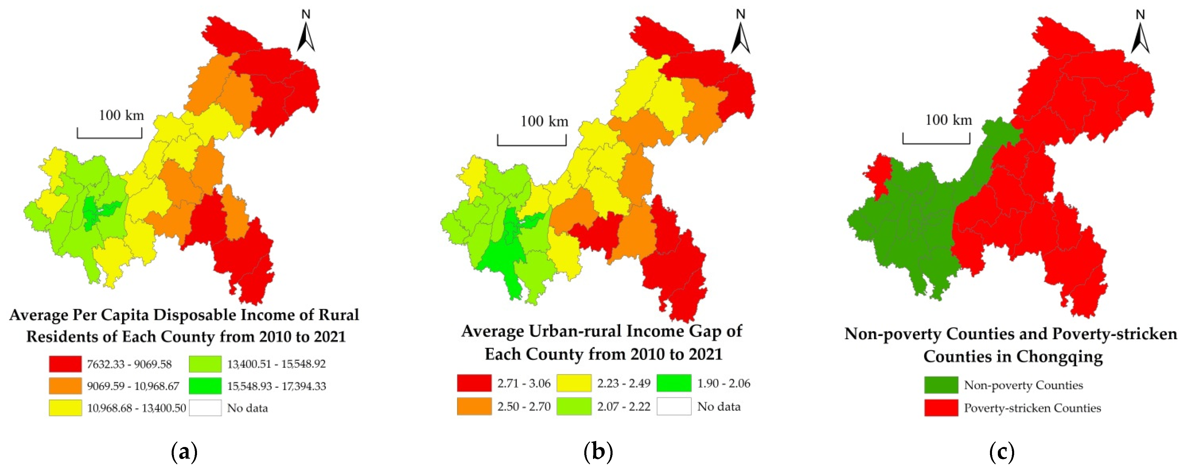
Income ratios in urban and rural Chongqing show spatial self-relevance and positive agglomeration, with lower ratios in the west and higher ratios in the north-east and south. In addition, the URIG in Chongqing is closely related to the PCDI of rural residents, showing a very obvious negative correlation; it also showed the trend of “poverty-stricken counties > non-poverty-stricken counties”.

(2)

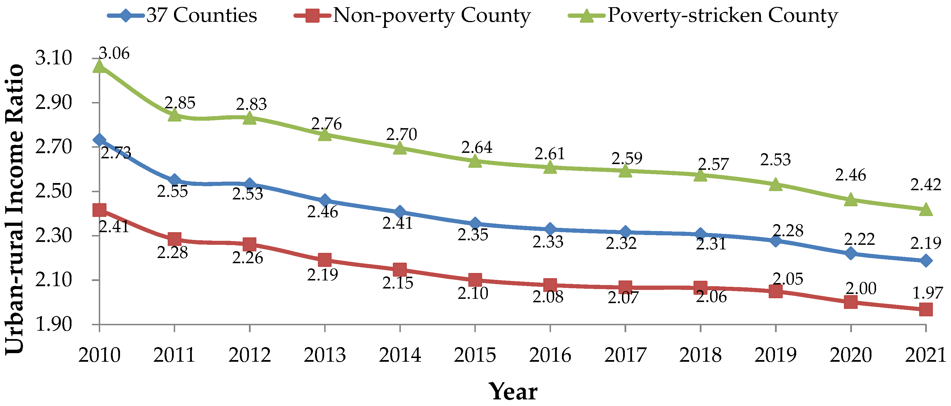
In general, the URIG in all counties of Chongqing has shown a declining annual trend. Although the URIG in poverty-stricken counties is generally high, the ratio of decline is slightly higher than that in non-poverty-stricken counties.

(3)

The outcomes of our analysis of the influencing factors reveal that the level of fixed assets investment, the per capita spending of public funds, the proportion of rural employees, the proportion of grain sowing, the amount of agricultural fertilizer applied per unit area, the proportion of real estate development investment, and population density variables are important factors of the URIG in Chongqing. The raise of the level of fixed assets investment, per capita public spending of public funds, the proportion of rural employees, the amount of agricultural fertilizer applied per unit area, and the proportion of investment in real estate development can considerably narrow the URIG. Meanwhile, increases in the proportion of grain sowing and population density have a notable inhibitory impact on narrowing the URIG. Furthermore, the effects of the aforementioned causes obviously differ for poverty-stricken and non-poverty-stricken counties.

(4)

The relevant factors’ spillover effects demonstrate that there are obvious spillover effects of the level of secondary industry development, the fixed assets investment level, the proportion of real estate development investment, and population density in constraining the narrowing of the URIG in non-poverty-stricken counties, but they also have obvious spillover impacts such as promoting the narrowing of the URIG in non-poverty-stricken counties. The proportion of grain sown clearly has a detrimental spillover effect in constraining the narrowing of the URIG, and non-poverty-stricken counties have a greater impact.

The analysis of the spatio-temporal evolution, spillover effects, and influencing variables of the URIG in Chongqing provides a foundation for policymakers to formulate measures to lower the URIG and to promote a coordinated urban–rural development strategy. Overall, the findings of this article can provide useful references for the development of urban and rural areas in Chongqing and indeed in China, enabling a reduction of the PCDI and the more effective implementation of the rural revitalization strategy and the urban–rural integration development strategy.

References

- Yang, R.Y.; Zhong, C.B.; Yang, Z.S.; Yang, S.Q. Can the Targeted Poverty Alleviation Policy Really Increase the Income of Rural Residents? An Empirical Test Based on 129 Counties in Yunnan Province. Nankai Econ. Stud. 2023, 39, 8. [Google Scholar]
- Yang, R.Y.; Yang, Z.S. Can the Sorghum Planting Industry in Less-Favoured Areas Promote the Income Increase of Farmers? An Empirical Study of Survey Data from 901 Samples in Luquan County. Agriculture 2022, 12, 2107. [Google Scholar] [CrossRef]
- Ma, X.; Wang, F.R.; Chen, J.D.; Zhang, Y. The income gap between urban and rural residents in China: Since 1978. Comput. Econ. 2018, 52, 1153–1174. [Google Scholar] [CrossRef]
- Yang, R.Y.; Zhong, C.B.; Yang, Z.S.; Wu, Q.J. Analysis on the Effect of the Targeted Poverty Alleviation Policy on Narrowing the Urban-Rural Income Gap: An Empirical Test Based on 124 Counties in Yunnan Province. Sustainability 2022, 14, 12560. [Google Scholar] [CrossRef]
- Sicular, T.; Yue, X.; Gustafsson, B.; Li, S. The urban-rural income gap and inequality in China. Rev. Income Wealth 2007, 53, 93–126. [Google Scholar] [CrossRef]
- Li, S.; Luo, C.L. Re-estimating the income gap between urban and rural households in China. J. Peking Univ. Philos. Soc. Sci. 2007, 44, 111–120. [Google Scholar]
- National Bureau of Statistics of the People’s Republic of China. China Statistical Yearbook 2021, 1st ed.; China Statistics Press: Beijing, China, 2021. [Google Scholar]
- Guo, Y.; Li, J.J.; Du, Z.X. Trends of urban-rural income gap: International experience and its implications for China. World Agric. 2022, 6, 5–17. [Google Scholar]
- Yang, Z.S.; Yang, R.Y.; Liu, F.L. Spatio-temporal evolution and influencing factors of urban–rural income gap in Yunnan province based on poverty classification. Geogr. Res. 2021, 40, 2252–2271. [Google Scholar]
- Xinhua News Agency. Premier Li Keqiang Attended the Press Conference and Answered Questions from Chinese and Foreign Journalists. Available online: http://www.gov.cn/premier/2020-05/29/content_5515798.htm#allContent (accessed on 29 May 2020).
- Ge, D.Z.; Long, H.L. Rural spatial governance and urban-rural integration development. Acta Geogr. Sin. 2020, 75, 1272–1286. [Google Scholar]
- Zhao, X.L. Five characteristics in the change of income gap in China. Econ. Rev. J. 2004, 20, 16–18. [Google Scholar]
- He, R.W. Urban-rural integration and rural revitalization: Theory, mechanism and implementation. Geogr. Res. 2018, 37, 2127–2140. [Google Scholar]
- Zhang, Y.N.; Long, H.L.; Ma, L.; Tu, S.S.; Chen, K.Q. Research progress of urban-rural relations and its implications for rural revitalization. Geogr. Res. 2019, 38, 578–594. [Google Scholar]
- Li, Y.H.; Yan, J.Y.; Song, C.Y. Rural revitalization and sustainable development: Typical case analysis and its enlightenments. Geogr. Res. 2019, 38, 595–604. [Google Scholar]
- Molero-Simarro, R. Inequality in China revisited. The effect of functional distribution of income on urban top incomes, the urban–rural gap and the Gini index, 1978–2015. China Econ. Rev 2017, 42, 101–117. [Google Scholar] [CrossRef]
- Colin, C. Conditions of Economic Progress, 1st ed.; Macmillan: London, UK, 1940. [Google Scholar]
- David, R. The Principles of Political Economy and Taxation, 1st ed.; Dover Publications: New York, NY, USA, 2004. [Google Scholar]
- Kuznets, S. Economic growth and income inequality. Am. Econ. Rev. 1955, 45, 42–48. [Google Scholar]
- Adelman, I.; Morris, C.T. Economic Growth and Social Equality in Development Country, 1st ed.; Stanford University Press: Palo Alto, CA, USA, 1973. [Google Scholar]
- Ahiuwalia, M. Inequality, poverty and development. J. Dev. Econ. 1976, 3, 307–342. [Google Scholar] [CrossRef]
- Anand, S.; Kanbur, S.M.R. Inequality and development: A critique. J. Dev. Econ. 1993, 41, 19–43. [Google Scholar] [CrossRef]
- Tunali, C.B.; Yilanci, V. Are per papita incomes of MENA countries converging or diverging? Stat. Mech. Its Appl. 2010, 21, 4855–4862. [Google Scholar] [CrossRef]
- Roland, B. Inequality and growth. NBER Macroecon. Annu. 1996, 11, 11–92. [Google Scholar]
- Klaus, D.; Lyn, S. New ways of looking at old issues: Inequality and growth. J. Dev. Econ. 1998, 57, 259–287. [Google Scholar]
- Piketty, T. The dynamics of the wealth distribution and the interest rate with credit rationing. Rev. Econ. Stud. 1997, 64, 173–189. [Google Scholar] [CrossRef]
- Fei, J.C.H.; Ranis, G.; Kuo, S.W.Y. Growth with Equality; Oxford University Press: London, UK, 1979. [Google Scholar]
- Fields, G.S. Decomposing LDC Inequalities. Oxf. Econ. Pap. New Ser. 1979, 31, 437–459. [Google Scholar] [CrossRef]
- Liu, J.X.; Li, X.Q.; Liu, S.T.; Rahman, S.; Sriboonchitta, S. Addressing Rural–Urban Income Gap in China through Farmers’ Education and Agricultural Productivity Growth via Mediation and Interaction Effects. Agriculture 2022, 12, 1920. [Google Scholar] [CrossRef]
- Wang, S.P.; Ouyang, Z.G. The threshold effect of China’s urban-rural income inequality on real economic growth. Soc. Sci. China 2008, 29, 54–66+205. [Google Scholar]
- Castello, A.; Domenech, R. Human capital inequality and economic growth: Some new evidence. Econ. J. 2002, 112, 187–200. [Google Scholar] [CrossRef]
- Knowles, S. Inequality and economic growth: The empirical relationship reconsidered in the light of comparable data. J. Dev. Stud. 2005, 41, 135–159. [Google Scholar] [CrossRef]
- Li, H.; Zou, H. Income inequality is not harmful for growth: Theory and evidence. Rev. Dev. Econ. 1998, 2, 318–334. [Google Scholar] [CrossRef]
- Forbes, K.J. A reassessment of the relationship between inequality and growth. Am. Econ. Rev. 2000, 90, 869–887. [Google Scholar] [CrossRef]
- Li, Y.Y.; Wang, C. Can centralized fiscal reform narrow the gap between urban and rural areas?—Evidence based on a quasi-natural experiment of “the village-finance-supervised-by-county”. Manag. World 2020, 36, 113–130. [Google Scholar]
- Wen, T.; Ran, G.H.; Xiong, D.P. Financial development and the income growth of farmer in China. Econ. Res. J. 2005, 51, 30–43. [Google Scholar]
- Zhang, S.H.; Liu, J. Is the targeted poverty-relief policy narrowing the income gap between the urban and rural areas?—An empirical study based on spatial panel data. J. Xinjiang Univ. Philos. Humanit. Soc. Sci. 2018, 46, 1–9. [Google Scholar]
- Liu, M.H.; Li, J.W.; Li, Q. Impact of targeted poverty alleviation on the urban-rural household income gap—A case study of shanxi province. Chin. J. Agric. Resour. Reg. Plan. 2020, 41, 228–237. [Google Scholar]
- Wan, H.Y.; Li, S. The effects of household registration system discrimination on urban-rural income inequality in China. Econ. Res. J. 2013, 48, 43–55. [Google Scholar]
- Zou, C.; Liu, J.; Liu, B.; Zheng, X.; Fang, Y. Evaluating poverty alleviation by relocation under the link policy: A case study from Tongyu County, Jilin Province in China. Sustainability 2019, 11, 5061. [Google Scholar] [CrossRef]
- Li, G. A Study on the Relationship between industrial structure and urban-rural income gap in the Yangtze River Economic Belt: An empirical test based on panel data. Inq. Into Econ. Issues 2019, 40, 72–77. [Google Scholar]
- Cheng, Y.H. China’s overall gini coefficient since reform and its decomposition by rural and urban areas since reform and opening-up. Soc. Sci. China 2007, 28, 45–60+205. [Google Scholar]
- Pan, J.H. Spatiotemporal pattern of urban-rural income gap of prefecture level cities or above in China. Econ. Geogr. 2014, 34, 60–67. [Google Scholar]
- Sun, X.Y.; Xu, Y.; Liu, Y.H. Residents’ income disparity and spatial difference in China. Econ. Geogr. 2015, 35, 18–25, 42. [Google Scholar]
- Chen, F.; Yu, T.H.; Wang, H.P. Analysis on the degree of urban-rural income polarization and its changes of temporal-spatial characteristics in central China. Hum. Geogr. 2012, 27, 104–109. [Google Scholar]
- Ding, Z.W.; Zhang, G.S.; Wang, F.Z. Spatial-temporal differentiation of urban-rural income in Central Plains Region at different scales. Geogr. Res. 2015, 34, 131–148. [Google Scholar]
- Zuo, Y.H. The study of reason for urban-rural Income gap in China: Based on the angel of income sources. Econ. Probl. 2011, 33, 40–43. [Google Scholar]
- Sun, J.S.; Huang, Q.H. Study on main influencing factors and contribution rate of income gap between urban and rural residents of China: Based on the data analysis of 6937 residents questionnaires from 31 provinces. Econ. Theory Bus. Manag. 2013, 33, 5–16. [Google Scholar]
- Wu, X.L.; Liu, Z.Y. The factors that affect the income gap between urban and rural areas of china: Based on the provincincial Panel Data from 2002 to 2011. Mod. Econ. Sci. 2014, 36, 46–54, 125–126. [Google Scholar]
- Li, J.J.; Mi, W.B.; Song, Y.Y.; Zhou, R.R.; Yang, R. Spatial-temporal differentiation and factors of urban-rural income gap in Ningxia. Res. Agric. Mod. 2016, 37, 785–793. [Google Scholar]
- Jiang, X.J.; Yang, Q.S.; Zhang, Y.; Wang, X.Y.; Liu, J.; Liu, J. Spatiotemporal differentiation and influencing factors of urban-rural income gap in northeast China based on multi-scale. Mod. Urban Res. 2019, 26, 109–118. [Google Scholar]
- Song, J. An empirical analysis on the influencing factors of urban-rural income gap in Hebei province. China Econ. Trade Her. 2019, 3, 92–94. [Google Scholar]
- Wang, N.; Wang, X. Analysis on the causes of the urban-rural income gap widening year by year in Yunnan province. Econ. Trade 2018, 4, 61+63. [Google Scholar]
- Brief Introduction of Chongqing. Available online: https://www.cq.gov.cn/zjcq/sqgk/cqsq/202302/t20230210_11593093.html (accessed on 10 February 2023).
- The Main Data of the Seventh National Population Census in Chongqing. Available online: http://tjj.cq.gov.cn/zwgk_233/fdzdgknr/tjxx/sjjd_55469/202105/t20210513_9277447.html (accessed on 13 May 2021).
- Survey Office in Chongqing, National Bureau of Statistics of the People’s Republic of China, Chongqing Municipal Bureau of Statistics. Chongqing Survey Yearbook 2022, 1st ed.; China Statistics Press: Beijing, China, 2022. [Google Scholar]
- Yang, R.Y.; Zhong, C.B. Analysis on Spatio-Temporal Evolution and Influencing Factors of Air Quality Index (AQI) in China. Toxics 2022, 10, 712. [Google Scholar] [CrossRef]
- Moran, P. Notes on Continuous Stochastic Phenomena. Biometrika 1950, 37, 17–23. [Google Scholar] [CrossRef]
- Elhorst, J.P. Spatial Econometrics: From Cross-Sectional Data to Spatial Panels, 1st ed.; Springer: Berlin/Heidelberg, Germany, 2014. [Google Scholar]
- Wang, D. Has Electronic Commerce Growth Narrowed the Urban–Rural Income Gap? The Intermediary Effect of the Technological Innovation. Sustainability 2023, 15, 6339. [Google Scholar] [CrossRef]
- Chen, T.W.; Zhang, Z.B. Can the Low-Carbon Transition Impact the Urban–Rural Income Gap? Empirical Evidence from the Low-Carbon City Pilot Policy. Sustainability 2023, 15, 5726. [Google Scholar] [CrossRef]
- Liu, P.J.; Zhang, Y.T.; Zhou, S.Q. Has Digital Financial Inclusion Narrowed the Urban–Rural Income Gap? A Study of the Spatial Influence Mechanism Based on Data from China. Sustainability 2023, 15, 3548. [Google Scholar] [CrossRef]
- Xiong, M.Z.; Li, W.Q.; Teo, B.S.X.; Othman, J. Can China’s Digital Inclusive Finance Alleviate Rural Poverty? An Empirical Analysis from the Perspective of Regional Economic Development and an Income Gap. Sustainability 2022, 14, 16984. [Google Scholar] [CrossRef]
- Zhang, S.H.; Sun, Y.; Yu, X.Z.; Zhang, Y.F. Geographical Indication, Agricultural Products Export and Urban–Rural Income Gap. Agriculture 2023, 13, 378. [Google Scholar] [CrossRef]
- Loewenstein, W.; Bender, D. Labor Market Failure, Capital Accumulation, Growth and Poverty Dynamics in Partially Formalised Economies: Why Developing Countries’ Growth Patterns are Different. SSRN Ecectrinic J. 2017. [Google Scholar] [CrossRef]
- Sadik-Zada, E.R. Distributional Bargaining and the Speed of Structural Change in the Petroleum Exporting Labor Surplus Economies. Eur. J. Dev. Res. 2020, 32, 51–98. [Google Scholar] [CrossRef]
- Sadik-Zada, E.R. Natural resources, technological progress, and economic modernization. Rev. Dev. Econ. 2021, 25, 381–404. [Google Scholar] [CrossRef]
- Harun, M.; Che, M.; Jalil, A. Public expenditure expansion and inter-ethnic and rural-urban income disparity. Procedia Econ. Financ. 2012, 1, 296–303. [Google Scholar] [CrossRef]
- Bauer, J. The internet and income inequality: Socio-economic challenges in a hyperconnected society. Telecommun. Policy 2018, 42, 333–343. [Google Scholar] [CrossRef]
- Yang, R.Y.; Zhong, C.B. Land Suitability Evaluation of Sorghum Planting in Luquan County of Jinsha River Dry and Hot Valley Based on the Perspective of Sustainable Development of Characteristic Poverty Alleviation Industry. Agriculture 2022, 12, 1852. [Google Scholar] [CrossRef]