Multi-Node Path Planning of Electric Tractor Based on Improved Whale Optimization Algorithm and Ant Colony Algorithm

Abstract

Under the “Double Carbon” background, the development of green agricultural machinery is very fast. An important factor that determines the performance of electric farm machinery is the endurance capacity, which is directly related to the running path of farm machinery. The optimized driving path can reduce the operating loss and extend the mileage of agricultural machinery, then multi-node path planning helps to improve the working efficiency of electric tractors. Ant Colony Optimization (ACO) is often used to solve multi-node path planning problems. However, ACO has some problems, such as poor global search ability, few initial pheromones, poor convergence, and weak optimization ability, which is not conducive to obtaining the optimal path. This paper proposes a multi-node path planning algorithm based on Improved Whale Optimized ACO, named IWOA-ACO. The algorithm first introduces reverse learning strategy, nonlinear convergence factor, and adaptive inertia weight factor to improve the global and local convergence ability. Then, an appropriate evaluation function is designed to evaluate the solving process and obtain the best fitting parameters of ACO. Finally, the optimal objective function, fast convergence, and stable operation requirements are achieved through the best fitting parameters to obtain the global path optimization. The simulation results show that in flat environment, the length and energy consumption of IWOA-ACO planned path are the same as those of PSO-ACO, and are 0.61% less than those of WOA-ACO. In addition, in bump environment, the length and energy consumption of IWOA-ACO planned path are 1.91% and 4.32% less than those of PSO-ACO, and are 1.95% and 1.25% less than those of WOA-ACO. Therefore, it is helpful to improve the operating efficiency along with the endurance of electric tractors, which has practical application value.

1. Introduction

Based on the needs of large agricultural bases in Xinjiang and the development of facility agriculture, agricultural machinery has been widely used. As a new type of agricultural machinery, the electric tractor has the advantages of low pollution, low noise, high efficiency, easy operation, etc. [1]. In recent years, it has been gradually applied to agricultural production [2,3]. From the reduction in loss and the improvement in endurance, we need to plan the optimal path to improve efficiency of electric tractors.

Multi-node path planning refers to the path after traversing all nodes in a certain area, starting from a node, with the set of optimal operation rules. This is an increasingly important area in automated production includes plant protection and farmland leveling [4,5], as well as tractor path planning [6]. Ref. [7] proposed a path planning and tracking control method, which was helpful for vehicle collision-free driving. Ref. [8] proposed a tractor path planning method applied in complex environment, which improved the tractor operation efficiency and coverage. In recent years, intelligent algorithm is a major area of interest within the field of multi-node path planning [9,10,11], such as ACO algorithm, genetic algorithm (GA), Particle Swarm Optimization (PSO), etc. Ref. [12] proposed an improved ant colony algorithm based on the adaptive volatile coefficient for the traveling salesman problems. Ref. [13] proposed a parallel ant colony algorithm for multi-node path planning of facility greenhouse robots. Ref. [14] proposed ant colony optimization algorithm variants to increase the probability of the algorithm to find the object. Ref. [15] proposed an improved ant colony optimization algorithm to solve the traveling salesman problem. Ref. [16] proposed an improved particle swarm optimization for multi-node path planning. Ref. [17] proposed GA for the traveling salesman problems. As the bionic ant colony foraging behavior adopted by ACO is similar to path planning, ACO is a commonly used algorithm to solve the multi-node path planning problem. When applying ACO to solving specific problems, it is possible to set the iteration rules of the algorithm parameters in a targeted way. However, ACO requires many parameters, and it is difficult to determine the optimal fitting combination of parameters. Therefore, it is easy for the algorithm to fall into local optimal solution, which is not conducive to obtaining the optimal path.

The Whale Optimization Algorithm (WOA) is an intelligent algorithm proposed by Australian scholars [18] which simulates the foraging behavior of whales to solve the objective function. WOA has the advantages of small number of setting parameters and strong convergence performance; however, it easily falls into local optimum and has low convergence accuracy. In recent years, a number of researchers have sought to improve WOA. References proposed improved whale optimization algorithms based on elite backward learning [19], the crossover and mutation operations [20], nonlinear convergence factor [21,22,23], and adaptive weighting factor [22,23], respectively, which balance between global and local convergence capability and enhance the diversity of the initial solution. Therefore, WOA has the possibility to further optimize population initialization and iteration rules to improve algorithm performance. However, a major problem with those is the complexity of optimization algorithm logic, which reduces the operational efficiency of the algorithm.

The main contributions of this paper are as follows:

• This paper proposes a fusion improved Whale Optimization Algorithm and Ant Colony algorithm, named IWOA-ACO, to plan the multi-node path of the electric tractor by optimizing the parameters of ACO. At the same time, IWOA introduces reverse learning strategy, nonlinear convergence factor and adaptive inertia weighting factor to balance between global and local convergence capability of it and enhance the diversity of the initial solution. Then, IWOA-ACO improves the evaluation function to ensure accurate evaluation of ACO performance during iteration. The block diagram of IWOA-ACO is shown in Figure 1.

2.

The operation node data of cultivated land environment in Xinjiang is taken and as an example, the experimental results show that IWOA-ACO algorithm can optimize ACO setting parameters to plan the optimal path of electric tractor, which is better than WOA-ACO and PSO-ACO in path length and energy consumption. Moreover, considering the flat terrain of Xinjiang, this paper constructs a bump environment model and conducts simulation experiments to reflect the universality of IWOA-ACO algorithm. In addition, the experimental results show that the length and energy consumption of the planned path of the algorithm is still better than those of WOA-ACO and PSO-ACO, reflecting the good value of the algorithm.

In a word, we propose an IWOA-ACO algorithm to plan a path with better path length and energy consumption. Based on the experimental analysis of complex nodes and experimental fields in Xinjiang, the path length and energy consumption of electric tractors planned by IWOA-ACO are better than those of WOA-ACO and PSO-ACO, thus improving the operating efficiency and endurance level of electric tractors.

2. Methods

2.1. Analysis of ACO

This section briefly introduces the operation principle of ACO algorithm and the impact of the main parameters on the algorithm performance. Aiming at the iteration redundancy problem that may be caused by setting an excessively high maximum iteration number of the algorithm, the Iteration Early Termination Strategy (IETS) is introduced to enhance the operational efficiency of the algorithm.

2.1.1. The Introduction of ACO

Ant foraging is a group behavior. In the process of foraging, ants will release volatile pheromones and perceive the residual pheromone concentration released by after other ones. Ants use roulette strategy when choosing the path, and will prioritize the path with short path and high pheromone concentration, which constitutes a positive feedback mechanism. After a period of time, the ant colony will choose an optimal path. The state transition function is shown by

$$P_{ij}^{t_{\mathrm{ACO}}}=\left\{\begin{array}{c}\frac{T{a}_{ij}{(t_{\mathrm{ACO}})}^{\alpha }E{t}_{ij}{(t_{\mathrm{ACO}})}^{\beta }}{{\displaystyle \sum _{t_{\mathrm{ACO}}\in allow(t_{\mathrm{ACO}},i)}T{a}_{ij}{(t_{\mathrm{ACO}})}^{\alpha }E{t}_{ij}{(t_{\mathrm{ACO}})}^{\beta }}},j\in allow(t_{\mathrm{ACO}},i)\\ 0,j\notin allow(t_{\mathrm{ACO}},i)\end{array}\right.$$

(1)

where t_ACO is the current iteration, $P_{ij}^{t_{\mathrm{ACO}}}$ is the state transition function, β is the heuristic function importance factor, α is the pheromone importance factor, i and j are the adjacent nodes, and allow(t_ACO,i) is the node that has not been accessed. Ta_ij(t_ACO) is pheromone concentration, as presented in Equation (2). Et_ij(t_ACO) is heuristic function, as presented in Equation (3).

$$T{a}_{ij}(t_{\mathrm{ACO}})=(1-rh)T{a}_{ij}(t_{\mathrm{ACO}}-1)+\Delta T{a}_{ij}(t_{\mathrm{ACO}})$$

(2)

where rh is the pheromone concentration volatilization factor, and ∆Ta_ij(t_ACO) is the new increment of pheromone on the path, which is related to whether ants pass through the path.

$$E{t}_{ij}(t_{\mathrm{ACO}})=\frac{1}{Di{s}_{ij}}$$

(3)

where Dis_ij is the European distance through the path.

When researchers apply the ant colony algorithm to specific problems, the main parameters to be set are α, β, rh and the ant quantity, such as m. This paper analyzes the impact of four parameters on the performance of ACO algorithm as follows [24]:

• α and β influence $P_{ij}^{t_{\mathrm{ACO}}}$ together. α reflects the importance of the ant colony to the existing pheromone when searching the path, and β reflects the degree to which the ant colony pays attention to the local shortest path when searching the path. When the setting values of α and β are large, the local convergence ability of the algorithm is strong. On the contrary, the algorithm has strong global convergence.
• rh affects the pheromone concentration level, thus affecting $P_{ij}^{t_{\mathrm{ACO}}}$. When the setting value of rh is large, the pheromone concentration on the path is low, and the positive feedback effect is weakened, so the algorithm has strong global convergence ability, but the convergence speed of the algorithm is slow. On the contrary, the pheromone concentration on the path is high, and the positive feedback effect is enhanced, so the algorithm converges quickly, but it easily falls into the local optimal solution.
• m affects the convergence ability and running speed of the algorithm. When the setting value of m is large, the global convergence of the algorithm is good, but the running speed is slow. On the contrary, the running speed of the algorithm is fast, but the convergence performance is poor, and it easily falls into the local optimal solution.

2.1.2. The Introduction of IETS

In ACO algorithm, when the set number of iteration terminations is larger than the solution problem, multiple iterations will have the same value at the end of the iteration, reducing the efficiency of the algorithm. This paper introduces IETS: when the iterative solution reaches the set value t_set with the same number of consecutive times t₀ and the iterative solution is less than the set value x_set, the iteration is terminated. Otherwise, the iteration will continue until the maximum iteration period t_max is met. The flowchart of IETS is shown in Figure 2.

2.2. Analysis of IWOA

This section introduces the operating principle of IWOA. Test functions are used to verify the operation performance of IWOA.

2.2.1. The Introduction of WOA

The operation logic of WOA originates from the foraging behavior of whales, including three search mechanisms: local optimization consisting of encirclement predation mechanism, spiral mechanism, and global optimization consisting of random search mechanism.

• Encirclement predation mechanism

The encirclement predation mechanism originates from the behavior of whales to identify and encircle their prey. The location of whales closest to their prey can be regarded as a local optimal solution, and other whales converge to the local optimal solution, as presented in Equations (4) and (5).

$$D=\left|C{X}^{*}\left(t\right)-X\left(t\right)\right|$$

(4)

$$X\left(t+1\right)=X^{*}\left(t\right)-AD$$

(5)

where X is the current whale position, X^* is the best whale location. A and C are coefficient vectors, as presented in Equations (6) and (7).

$$A=2ar-a=a(2r-1)$$

(6)

$$C=2r$$

(7)

where r is a random variable belonging to [0, 1], a is the linearly decreasing convergence factor from 2 to 0.

2.

Spiral mechanism

The spiral mechanism is based on the fact that whales emit bubbles and move to their prey in a spiral motion in the process of foraging, as presented in Equation (8).

$$X\left(t+1\right)=D{e}^{bl}\cos \left(2\pi l\right)+X^{*}\left(t\right)$$

(8)

where b is a constant, l is a random variable belonging to [0, 1].

3.

Random search mechanism

The random search mechanism is based on the fact that whales not only approach the nearest whale location from their prey, but also randomly select other whale locations in the population to search, as presented in Equations (9) and (10).

$$D^{*}=\left|C{X}_{rand}\left(t\right)-X\left(t\right)\right|$$

(9)

$$X\left(t+1\right)=X_{rand}(t)-A{D}^{*}$$

(10)

where X_rand is the position of whales randomly selected in the population.

The operation logic of the three search mechanisms is as follows:

p = rand(0,1)

if  p < 0.5

if |A| < 1

Encirclement predation, (5)

else

Random search, (10)

end

else

Spiral, (8)

end

2.2.2. Analysis of IWOA

In order to improve the convergence performance of WOA, this paper optimizes WOA in three aspects to obtain IWOA.

• Population initialization with reverse learning strategy (PIRL)

The quality of the initial population affects the convergence speed and accuracy of the algorithm, and high-quality initial population is conducive to the rapid convergence of the algorithm. In WOA, the initialization of the population is completely random, which has the advantage of ensuring the diversity of the initial population, but the quality of the initial population generated by this scheme is not high. To ensure the diversity of the initial population and improve the quality of the initial population, PIRL is introduced in this paper. The strategy steps are as follows:

• Establish a random initial population, and analyze the position of individuals in the random initial population in turn.
• Set a random variable p belonging to [0, 1]. Adopt reverse learning strategy if p ≥ 0.3. Assume that the position of individual r in the d-dimensional space is $X_r\left(1,2,\dots ,d\right)$, then the corresponding reverse individual is ${\tilde{X}}_r\left(1,2,\dots ,d\right)$, as presented in Equation (11).

$${\tilde{X}}_r\left(k\right)=L\left(k\right)+U\left(k\right)-X_r\left(k\right)$$

(11)

where L(k) and U(k) are the boundaries of population space. The fitness values of individuals $X_r\left(1,2,\dots ,d\right)$ and ${\tilde{X}}_r\left(1,2,\dots ,d\right)$ are calculated, respectively, and the individual with better fitness is retained as the final initial population.

• Do not adopt reverse learning strategy if p < 0.3. The individual $X_r\left(1,2,\dots ,d\right)$ is retained as the final initial population.

2.

Nonlinear convergence factor.

After analyzing the operation logic of the three search mechanisms, the paper concludes that the size of |A| determines the global and local search of the algorithm. According to Equation (6), the size of convergence factor a determines the size of |A|. In WOA, convergence factor a is linearly decreasing. Therefore, when the number of iterations is greater than half of the maximum number of iterations, a < 1. In the middle of iteration, |A| drops to a low value too early, so that WOA changes from global search to local search too early, increasing the possibility of the algorithm falling into the local optimal solution.

In order to better balance the ability of global search and local search of the algorithm and make the algorithm turn to local search after full global search, exponential nonlinear convergence factor a* is introduced in this paper, as presented in Equation (12).

$$a*=\frac{-e^{\frac{t}{{\mathrm{T}}_{\max }}\ln 51}+51}{25}$$

(12)

where a* is the nonlinear convergence factor, T_max is the maximum number of iterations.

Assuming T_max = 50, the curve of a* is drawn as shown in Figure 3.

In the early and middle stages of the iteration process, the value of a* is kept at a high level to ensure the global search capability of the algorithm, and it decreases rapidly in the late iteration period to ensure that the algorithm focuses on local search.

3.

Adaptive inertia weighting factor

The idea of inertia weight factor is derived from PSO [25]. Individuals consider the impact of the current position when they move to the local optimal solution. In WOA, the value of inertia weight factor is always 1. In the early of iteration process, a large inertia weight factor is helpful to the global search of WOA. However, in the late iteration period, it causes the individual to pay too much attention to the current optimal solution position, so the algorithm easily falls into local optimization.

Therefore, this paper introduces adaptive inertial weighting factor w, as presented in Equation (13). In the early of iteration process, the global search ability of IWOA can be enhanced by the large value of w. In the late iteration period, the smaller value of w can reduce the dependence of individuals on the current optimal solution and avoid IWOA falling into the local optimal solution.

$$w=0.4{\left(\frac{t}{{\mathrm{T}}_{\max }}\right)}^2-0.8\frac{t}{{\mathrm{T}}_{\max }}+0.9$$

(13)

In IWOA, Equations (5) and (8) should be changed to Equations (14) and (15).

$$X\left(t+1\right)=wX*\left(t\right)-AD$$

(14)

$$X\left(t+1\right)=D{e}^{bl}\cos \left(2\pi l\right)+wX*\left(t\right)$$

(15)

2.2.3. Operation Steps of IWOA

IWOA is optimized in terms of population initialization and iteration parameters. The operation steps of IWOA are as follows:

• Set algorithm parameters, such as variable dimension, number of population individuals, and maximum number of iterations.
• Randomly initialize the population within the range of variable values.
• Establish initial population by PIRL and record the individual position with better fitness as the optimal position.
• The algorithm updates the location of individuals based on different search mechanisms. Set a random variable as p = rand (0,1). If p < 0.5 and |A| < 1, the algorithm individually updates their positions according to the encirclement predation mechanism, as in Equation (14). If p < 0.5 and |A| ≥ 1, individually update position according to the random search mechanism, as presented in Equation (10). If p ≥ 0.5, individually update position according to the spiral mechanism, as in Equation (15).
• The algorithm restricts the range of the updated position of the individuals, calculates the fitness values of those, and updates the optimal position.
• The algorithm judges whether the maximum number of iterations is reached. If so, it exits the iteration and outputs the optimal location and fitness value. If not, it returns to step (4) to continue iteration.

2.2.4. Performance Testing for IWOA

This paper selects four test functions to verify the performance of IWOA [26], as shown in

Table 1. Introduction to test functions.

Name	Expression	Dimension	Domain of Definition	Theoretical Optimal Value
Sphere	$F={\displaystyle \sum _{i=1}^n{x}_i^2}$	30	[−100, 100]	0
Quartic	$F=rand(0,1)+{\displaystyle \sum _{i=1}^{n}i{x}_i^4}$	30	[−1.28, 1.28]	0
Schwefel 2.26	$F={\displaystyle \sum _{i=1}^n-x_i\sin \sqrt{\left|x_i\right|}}$	30	[−500, 500]	−12,569
Rastrigin	$F={\displaystyle \sum _{i=1}^n\left[x_i^2-10\cos \left(2\pi x_i\right)+10\right]}$	30	[−5.12, 5.12]	0

. Then, this paper sets the population number as 40 and the maximum number of iterations as 100, and compares the performance of the three algorithms, including IWOA, WOA and PSO.

Sphere and Quartic are unimodal functions used to test the local search ability of those algorithms, and Schwefel 2.26 and Rastigin are multimodal functions used to test the global search ability of those algorithms. And the convergence curves of test functions are shown in Figure 4.

IWOA has converged to the optimal value in the 10th to 20th iterations, so IWOA is superior to WOA and PSO in convergence speed.

In order to better compare and analyze the performance of IWOA, this paper uses those algorithms to run each test function 30 times, and records the optimal values, the worst values and the standard deviation of the optimization results. The analysis of optimization results is shown in

Table 2. The analysis of optimization results.

Name	Statistic	IWOA	WOA	PSO	Optimal Algorithm
Sphere	Optimal value	6.66 × 10−40	4.83 × 10−17	478.21	IWOA
	Worst value	7.01 × 10−29	5.89 × 10−11	2296.15
	Standard deviation	1.30 × 10−29	1.06 × 10−11	407.98
Quartic	Optimal value	8.41 × 10−6	7.01 × 10−4	0.29	IWOA
	Worst value	2.22 × 10−3	5.81 × 10−2	1.85
	Standard deviation	5.02 × 10−4	1.15 × 10−2	0.45
Schwefel 2.26	Optimal value	−12,569.24	−12,318.02	−8677.97	IWOA
	Worst value	−10,600.90	−7422.42	−5034.17
	Standard deviation	453.58	1378.79	908.84
Rastrigin	Optimal value	0	0	73.14	IWOA
	Worst value	0	1.30 × 10−6	182.02
	Standard deviation	0	2.33 × 10−7	23.79

.

The optimal and the worst values of the function obtained by IWOA convergence are better than those of WOA and PSO, and the standard deviation of the data obtained by IWOA in 30 groups of tests is lower, so the performance of IWOA is more stable. In general, IWOA performs better than WOA and PSO in unimodal and multimodal test functions. Therefore, IWOA performs better in local search and global search, verifying the optimization effect.

2.3. Multi-Node Path Planning Problem of Electric Tractor

2.3.1. Analyze the Application Scenario

Multi-node path planning problem refers to the optimal path planning for multiple nodes in a certain area. The legal path is the path that starts from a node and traverses all other nodes. In agricultural production, the nodes are the marshal point of the harvested crops, and the electric tractor needs to traverse all the nodes in the region to collect all the harvested crops. In this paper, we employ a cultivated area, including node data and operating parameters of electric tractor, as the experimental object to verify the effectiveness of IWOA-ACO.

In order to exclude the influence of irrelevant factors on the experiment, we make the following assumptions:

• The path between nodes is a segment.
• Neglect the turning action of electric tractor at nodes.
• Neglect the air resistance of the electric tractor.
• Focus on the path length and energy consumption of electric tractors between nodes.

We choose the cultivated area located near 87.4 E and 44.3 N. The positions of 26 nodes in space are shown in Figure 5.

2.3.2. Kinematics Model of Electric Tractor

When the electric tractor travels between different operating points, it often travels at a low speed and at a constant speed. The energy loss in the operation of the electric tractor is mainly the energy consumed during travel. The force analysis of the electric tractor under different road conditions (flat ground and slope) [27] is shown in Figure 6.

When the electric tractor runs on the slope, the slope angle θ_i,j is shown in Equation (16). The path length of electric tractor traveling between nodes i and j is shown in Equation (17).

$${\theta }_{i,j}=\arctan \left(\frac{h_{i,j}}{s_{i,j}}\right)$$

(16)

$${\gamma }_{i,j}=\sqrt{s_{i,j}{}^2+h_{i,j}{}^2}$$

(17)

where γ_i,j is the path length between nodes, s_i,j is the horizontal distance between nodes, h_i,j is the height difference between nodes.

The mechanical expression of the electric tractor in uniform running is shown in Equation (18).

$$F_{\mathrm{q}}=\mathsf{\mu }\mathrm{G}\cos ({\theta }_{i,j})+\mathrm{G}\sin ({\theta }_{i,j})$$

(18)

where F_q is the driving force of power motor of electric tractor, μ is the friction coefficient of traveling road surface, G is the gravity of electric tractor.

The energy consumed by the motor during operation is shown in Equation (19).

$$Q_{i,j}=U{q}_{i,j}$$

(19)

where U is the input voltage of motor, q_i,j is the power consumed by the motor.

The driving force of the electric tractor during traveling is shown in Equation (20).

$$F_{\mathrm{q}}=\frac{T_{\mathrm{x}}{i}_{\mathrm{g}}{i}_0\mathsf{\eta }}{\mathrm{R}}=\frac{T_{\mathrm{t}}{i}_{\mathrm{g}}{i}_0\mathsf{\eta }}{\mathrm{R}}$$

(20)

where T_x is the output torque of planet carrier, i_g is the transmission speed ratio of electric tractor, i₀ is the differential speed ratio, η is the transmission efficiency; R is the wheel radius of electric tractor, T_t is the torque of motor, as shown in Equation (21).

$$T_{\mathrm{t}}=\frac{9550P}{n}$$

(21)

where n is the motor speed, P is the output power of motor.

The relationship between the traveling speed of the electric tractor v and the motor speed is shown in Equation (22).

$$v=\frac{0.377\mathrm{R}n}{i_{\mathrm{g}}{i}_0}$$

(22)

From Equations (16)–(22), the energy consumed by electric tractor Q_i,j when traveling between nodes i and j is shown in Equation (23).

$$Q_{i,j}=\frac{(\mathsf{\mu }\mathrm{G}\cos ({\theta }_{i,j})+\mathrm{G}\sin ({\theta }_{i,j}))s_{i,j}}{3.6\mathsf{\eta }\cos ({\theta }_{i,j})}$$

(23)

Regarding balance, from Equations (17) and (23), the kinematic function model of electric tractor is shown in Equation (24).

$$F_{\mathrm{kin}}=f({\gamma }_{i,j},Q_{i,j})$$

(24)

2.4. IWOA-ACO

The basic idea of IWOA-ACO is to use ACO to solve the optimal path of multiple nodes, and then use IWOA to optimize the operation parameters of ACO. There are two key problems when fusing IWOA and ACO algorithm. On the one hand, IWOA-ACO needs to set appropriate evaluation function to evaluate the solution process and results of ACO algorithm. On the other hand, IWOA-ACO needs to put ACO algorithm into IWOA iteration to solve the multi-node problem, and in IWOA iteration, input the four setting parameters mentioned in Section 2.1 to ACO algorithm.

An appropriate evaluation function is crucial for IWOA-ACO to optimize the parameters of ACO. The evaluation function should reflect the optimality, fast convergence and algorithm stability of the objective function of ACO for solving multi-node path planning. The evaluation function is shown in Equation (25).

$$y=k_1{f}_1+k_2{f}_2+k_3{f}_3+k_4{f}_4$$

(25)

where f₁ is the difference between the path length value obtained by ACO and the empirical optimal value of path length, as shown in Equation (26). f₂ is the difference between the energy consumption value obtained by ACO and the empirical optimal value of energy consumption, as shown in Equation (27). f₁ and f₂ represent the optimality of the algorithm for solving the objective function. f₃ is the iteration number of ACO, representing the fast convergence of the algorithm, as shown in Equation (28). f₄ is the standard deviation of the iterative data of ACO, representing the stability of the iterative data of the algorithm, as shown in Equation (29). k₁, k₂, k₃ and k₄ are the weight coefficients.

$$f_1=length-length\_\min$$

(26)

$$f_2=energy-energy\_\min$$

(27)

$$f_3={\displaystyle \sum length}$$

(28)

$$f_4=\delta (length)$$

(29)

The flow chart of IWOA-ACO is shown in Figure 7.

3. Results and Discussion

This section applies IWOA-ACO to solve the problem and analyzes the simulation results of flat and bump environment by the three algorithms so as to verify the performance of IWOA-ACO.

3.1. Simulation of Flat Environment

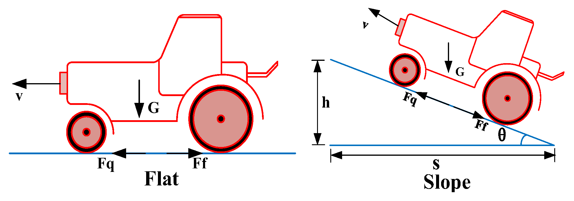
First, according to the analysis in Section 2.3.1, we need to extract the node data from the test field, and the experiment needs a planned optimal path for the electric tractor to traverse all nodes. Second, we need to set the relevant parameters of the electric tractor as follows: the friction coefficient of traveling road surface is 0.07, the gravity of electric tractor is 10,700, and the transmission efficiency is 0.85. Then, we need to unify the evaluation functions of the three algorithms into Equation (25), and unify the setting parameters as follows: the variable dimension is 4, the number of individuals in the population is 30, the maximum number of iterations is 50. Finally, in order to eliminate the impact of algorithm simulation environment on algorithm performance, we unify the simulation environment of the three algorithms as follows: Windows10 (64 bit), Core (TM) i7-8550U, CPU 1.80 GHz, 16 GB, MatlabR2017a.

In order to better analyze the operational performance of IWOA-ACO, this paper solves the node path planning problem as shown in Figure 5 with IWOA-ACO, WOA-ACO and PSO-ACO, compares the iteration curves of the evaluation functions of the three algorithms, and records the operation parameters of ACO algorithm, respectively.

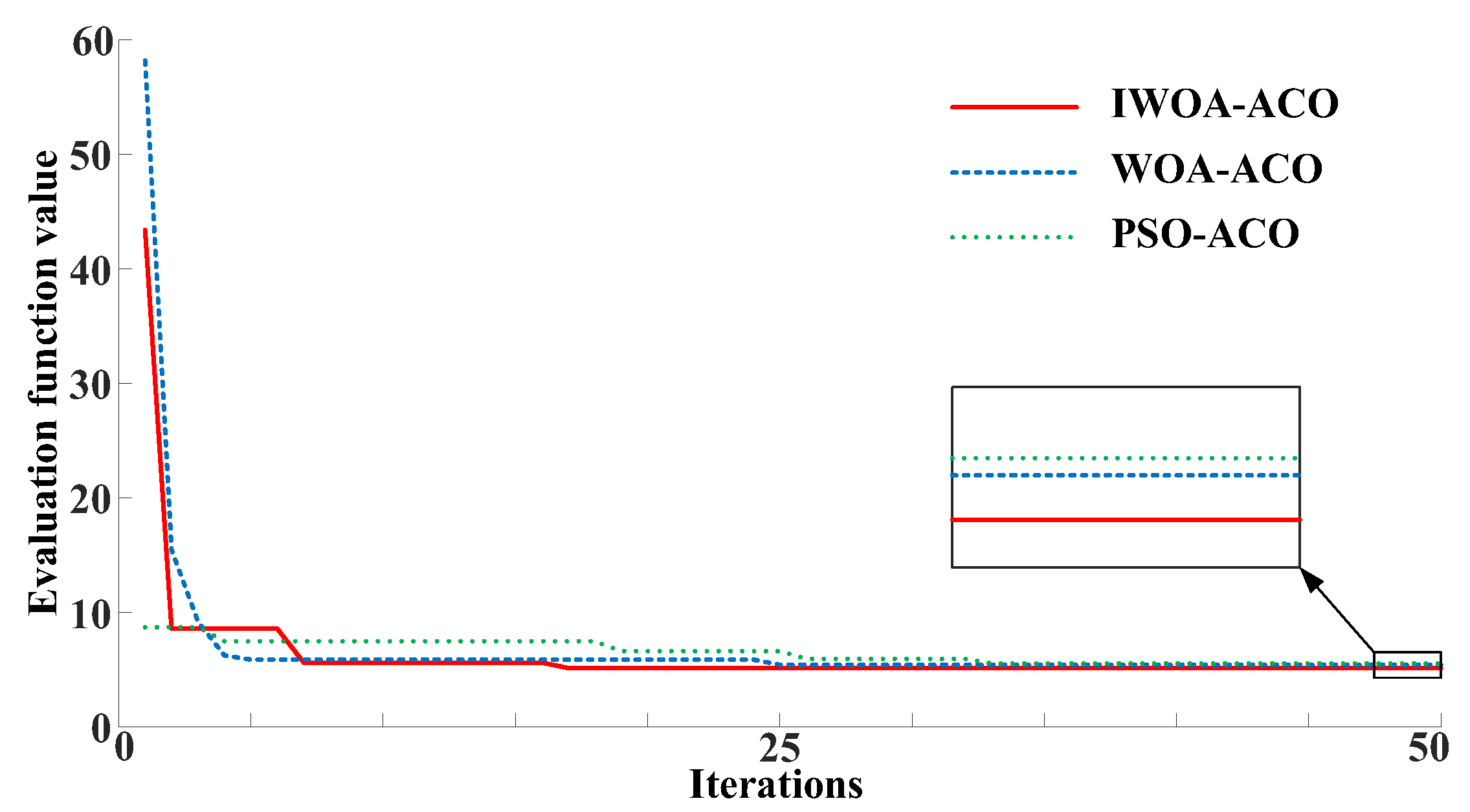
The convergence curve of the evaluation function corresponding to the three algorithms is shown in Figure 8. The parameter values of ACO obtained by convergence of three functions are shown in

Table 3. The parameter values of ACO in the simulation of flat environment.

Algorithm	m	rh	β	α
PSO-ACO	80	0.80	4.39	0.50
WOA-ACO	80	0.80	3.39	2.00
IWOA-ACO	80	0.80	5.00	0.50

. The convergence value of the evaluation function of IWOA-ACO is better than that of WOA-ACO and PSO-ACO.

Ref. [24] referred to the scheme of determining the parameter values of standard ACO algorithm by empirical method. In order to better verify the convergence performance of the IWOA-ACO algorithm, we employ the optimization scheme of the standard ACO algorithm as the control group in the comparison simulation. The parameter values of the algorithm are set according to Ref. [24]: m = 50, α = 1, β = 7 and rh = 0.3.

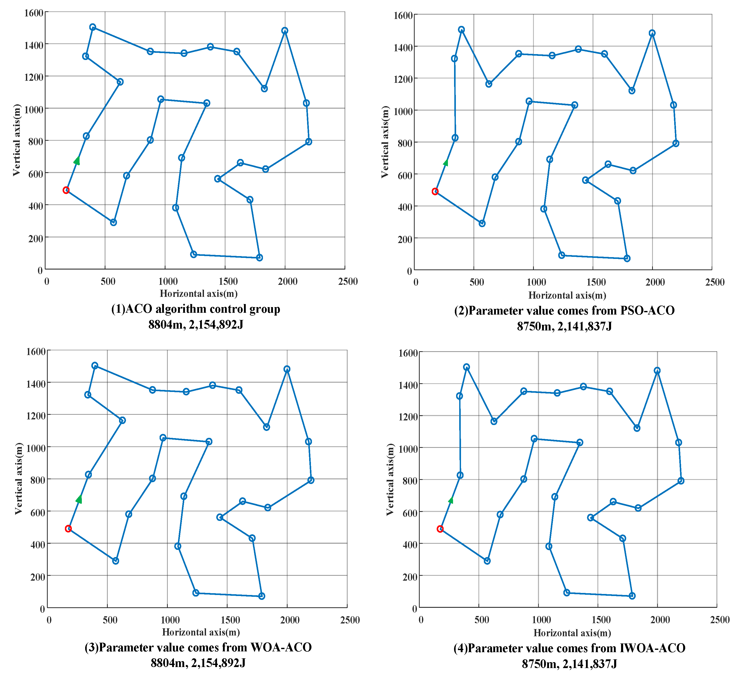
ACO plans the 26 node paths of the electric tractor according to the operation parameters in Table 3 and experience parameters. The generated path planning diagram is shown in Figure 9. This paper uses the iteration path length convergence curve to compare the convergence performance of ACO under different parameters, as shown in Figure 10.

3.2. Simulation of Bump Environment

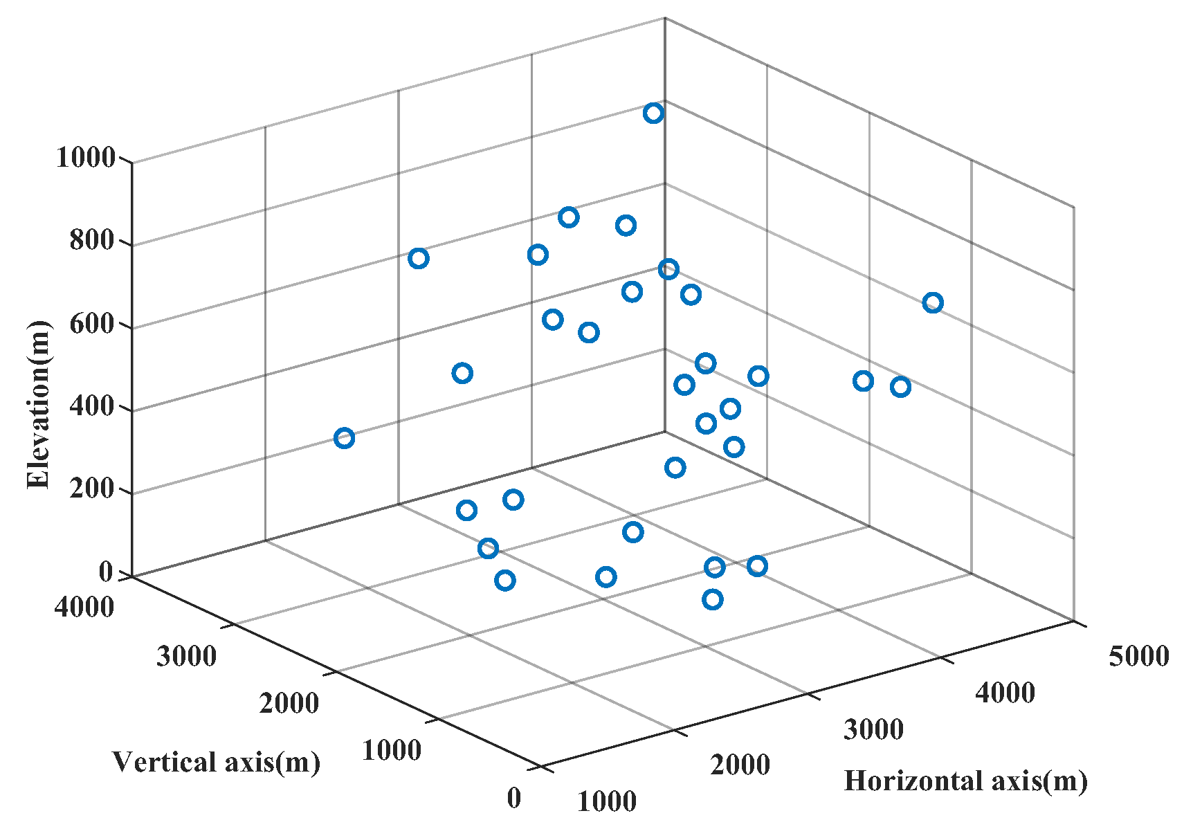
The cultivated land environment in Xinjiang is characterized by flat terrain [28,29]. Therefore, the node data in the cultivated area selected in this paper is approximately 2D. In order to further explore the adaptability of IWOA-ACO in the diversified cultivated land environment, we introduce the data of 31 nodes in the bump environment. The experimental steps and the parameters are set as shown in Section 3.1, and this paper compares the simulation results of the three algorithms. The positions of 31 nodes in space are shown in Figure 11.

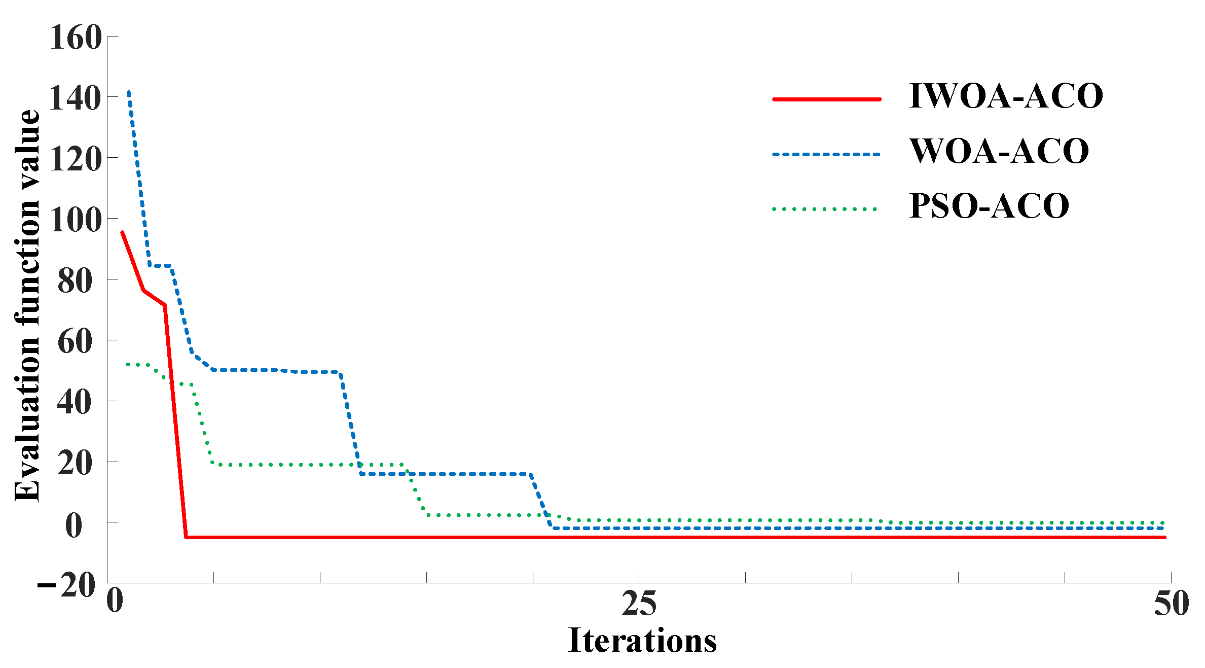
The convergence curve of the evaluation function corresponding to the three algorithms is shown in Figure 12. The parameter values of ACO obtained by convergence of three functions are shown in

Table 4. The parameter values of ACO in the simulation of bump environment.

Algorithm	m	rh	β	α
PSO-ACO	47	0.2	4.69	0.55
WOA-ACO	76	0.32	3.68	2
IWOA-ACO	72	0.78	2	0.83

. The convergence value of the evaluation function of IWOA-ACO is better than that of WOA-ACO and PSO-ACO. Moreover, the evaluation function value of IWOA-ACO can converge to the optimal value after five iterations, while WOA-ACO requires 20 iterations and PSO-ACO requires 15 iterations. It can be seen that the convergence performance of IWOA-ACO is better than that of WOA-ACO and PSO-ACO in solving the multi-node path planning problem.

As in Section 3.1, in order to better verify the convergence performance of the IWOA-ACO algorithm, we employ the optimization scheme of the standard ACO algorithm as the control group in the comparison simulation. The parameter values of the algorithm are m = 50, α = 1, β = 7 and rh = 0.3.

ACO plans the 31-node path of electric tractor based on the operating parameters obtained from the above three algorithms and experience parameters, and the resulting path planning diagram is shown in Figure 13. This paper uses the iterative path length convergence curve to compare the convergence performance of ACO under different parameters, as shown in Figure 14.

3.3. Discussion for Flat Environment Results

Based on Figure 9 and Figure 10, this paper analyzes the impact of ACO algorithm control group and the three parameter combinations shown in Table 3 on the performance of ACO as follows:

On the one hand, as far as the convergence speed of ACO algorithm is concerned, IWOA-ACO is equivalent to WOA-ACO and faster than PSO-ACO.

On the other hand, the path length planned by PSO-ACO is 8750 (m), and the energy consumed by electric tractor is 2,141,837 (J). The length and energy consumption of IWOA-ACO planned path are the same as those of PSO-ACO, and are 0.61% less than those of WOA-ACO and ACO algorithm control group (the value of the path length is 8804 m, and the value of the energy is 2,154,892 J). In the simulation of flat environment, the path length and energy consumption data of electric tractor are shown in

Table 5. The path length and energy consumption data in the simulation of flat environment.

Algorithm	ACO Control Group	PSO-ACO	WOA-ACO	IWOA-ACO
The path length (m)	8804	8750	8804	8750
	0%	−0.61%	0%	−0.61%
The energy (J)	2,154,892	2,141,837	2,154,892	2,141,837
	0%	−0.61%	0%	−0.61%

. It is worth mentioning that since the nodes are approximately distributed in 2D space, the energy consumed by the electric tractor is proportional to the path length.

In general, the path planned by IWOA-ACO for the electric tractor has the advantages of fast convergence speed of WOA-ACO and strong convergence ability of PSO-ACO, which is helpful for efficient operation of the electric tractor.

3.4. Discussion for Bump Environment Results

In the simulation of bump environment, the path length and energy consumption data of electric tractor are shown in

Table 6. The path length and energy consumption data in the simulation of bump environment.

Algorithm	ACO Control Group	PSO-ACO	WOA-ACO	IWOA-ACO
The path length (m)	19,395	19,420	19,428	19,057
	0%	+0.13%	+0.17%	−1.74%
The energy (J)	4,213,209	4,246,522	4,121,440	4,070,478
	0%	+0.79%	−2.18%	−3.39%

.

Based on Figure 13 and Figure 14, this paper analyzes the impact of the three parameter combinations shown in Table 4 on the performance of ACO as follows:

First of all, ACO, according to the parameters obtained from PSO-ACO, requires approximately 60 iterations to converge to the optimal value. The path length planned by the algorithm is 19,420 (m), and the energy consumed by electric tractor is 4,246,522 (J). The reason is that a small quantity of ants (the value is 47) leads to the slow convergence speed of the algorithm, and a small number of the pheromone concentration volatilization factor (the value is 0.2) leads to the local optimal solution of the algorithm.

In the second place, ACO, according to the parameters obtained from WOA-ACO, requires approximately 20 iterations to converge to the optimal value. The path length planned by the algorithm is 19,428 (m), and the energy consumed by electric tractor is 4,121,440 (J). The reason is that a large quantity of ants (the value is 76) leads to the fast convergence speed of the algorithm, but a small number of the pheromone concentration volatilization factor (the value is 0.32) leads to the local optimal solution of the algorithm.

Once more, ACO, according to the parameters obtained from IWOA-ACO, requires approximately 20 iterations to converge to the optimal value. The algorithm converges faster than the ACO algorithm with the parameters obtained from PSO-ACO, and approximates to the ACO algorithm with the parameters obtained from WOA-ACO. The path length planned by the algorithm is 19,057 (m), which is 1.91% less than that planned by the ACO algorithm with the parameters obtained from PSO-ACO and 1.95% less than that planned by the ACO algorithm with the parameters obtained from WOA-ACO. The energy consumed by electric tractor is 4,070,478 (J), which is 4.32% less than that optimized by the ACO algorithm with the parameters obtained from PSO-ACO and 1.25% less than that optimized by the ACO algorithm with the parameters obtained from WOA-ACO. In addition, the length and energy consumption of IWOA-ACO planned path are 1.74% and 3.39% less than those of ACO algorithm control group.

The reasons for the above results are as follows. On the one hand, a large quantity of ants (the value is 72) leads to the fast convergence speed of the algorithm and a large value of pheromone concentration volatilization factor (the value is 0.78) leads to good global convergence of the algorithm. On the other hand, the difference between the pheromone importance factor (the value is 0.83) and the heuristic function importance factor (the value is 2) is small, so that the algorithm can fully consider the pheromone concentration and heuristic function in the iterative process. Therefore, the algorithm can balance global and local searches.

However, IWOA-ACO has some limitations in practical application. On the one hand, IWOA-ACO can only obtain a set of set value parameters of ACO algorithm with good matching, but the ideal ACO parameter should be an adaptive function. On the other hand, affected by the fluctuation of ACO convergence results, the reliability of IWOA-ACO evaluation function has a negative correlation with the optimization time of the algorithm. We need to adjust the weight of evaluation function reliability and optimization time according to specific conditions.

4. Conclusions and Future Research

4.1. Conclusions

This paper proposes IWOA-ACO to plan the operation path of the electric tractor. IWOA introduces reverse learning strategy, nonlinear convergence factor and adaptive inertia weighting factor to balance between global and local convergence capability of it and enhance the diversity of the initial solution. At the same time, IWOA-ACO improves evaluation function to ensure accurate evaluation of ACO performance during iteration.

First of all, taking a cultivated land environment in Xinjiang as an example, IWOA-ACO is used to plan the optimal path for the electric tractor to traverse the crop concentration points. The simulation results show that the algorithm has the advantages of fast convergence speed and good global convergence performance, which is helpful to improve the working efficiency of the electric tractor. Furthermore, taking the complex nodes in a concave–convex environment as an example, the length and energy consumption of IWOA-ACO planned path are 1.91% and 4.32% less than those of PSO-ACO, and are 1.95% and 1.25% less than those of WOA-ACO. This verifies the strong adaptability of IWOA-ACO to various environments.

In conclusion, IWOA-ACO can reduce the length and energy consumption of the planned path, which improves the operational efficiency and endurance of the electric tractor and assists the development of green agricultural machinery.

4.2. Suggestions for Future Work

There is room for further progress in the research on obtaining optimization parameters of ACO algorithm. This paper makes a brief analysis of them to provide research ideas for follow-up researchers.

• As analyzed in Section 2.1.1, the ideal ACO parameter should not be a fixed value, but an adaptive function that is an iterative rule. In the research scheme proposed in this paper, IWOA-ACO algorithm can only obtain a set of set value parameters of ACO algorithm with good matching, but the step of obtaining the function from the set value parameters still needs to be completed by researchers. We propose that IWOA-ACO cannot directly derive the parameter iteration rules of ACO algorithm because of the limitations of its performance and dimensions. The analysis is as follows:

Assuming that the number of parameters to be determined by ACO algorithm is n_x, and the maximum number of iterations set by ACO algorithm when solving the path planning is m_x, the calculation dimension C_d of IWOA-ACO is as shown in Equation (30).

$$C_{\mathrm{d}}=n_{\mathrm{x}}{m}_{\mathrm{x}}$$

(30)

Taking the simulation in Section 3 as an example, the maximum number of iterations is m_x = 100. In ACO algorithm iteration, the ant quantity should be set as a constant. Therefore, the value of C_d should be C_d = 1 + 300 = 301. However, the value of C_d with the scheme adopted in this paper is C_d = 4.

In a word, this scheme, obtaining the adaptive functions directly from IWOA-ACO, has a large calculation dimension, which greatly increases the computational complexity of the algorithm. Therefore, the algorithm easily falls into the local optimal solution, and the operation effect may not be as good as that of the scheme adopted in this paper. In further research, it might be possible to use a better performance algorithm to achieve this scheme.

2.

As described in Section 2.4, in IWOA-ACO, the evaluation function is calculated by running the ACO algorithm only once under a set of parameter values. However, ACO algorithm, like GA, PSO, and WOA, belongs to intelligent algorithm, which has a high probability of obtaining the optimal value, but it cannot guarantee that every time it is the optimal value. If we aim to obtain a more reliable evaluation function, we need to allow ACO to run n_t times under each set of parameters to calculate the evaluation function by integrating the operation results. However, this will increase the running time of IWOA-ACO algorithm, as shown in Equation (31).

$$N_{\mathrm{T}}=t_{\mathrm{IWOA}-\mathrm{ACO}}{n}_{\mathrm{t}}$$

(31)

where t_IWOA-ACO is the time required for the scheme adopted in this paper which lets ACO run once under each set of parameters to calculate the evaluation function.

In a word, we realize that researchers can set the running times of the ACO algorithm n_t on the basis of measuring the running time of the IWOA-ACO algorithm N_T and the reliability of the evaluation function.