
The Influence of Soil Physical Properties on the Load Factor for Agricultural Tractors in Different Paddy Fields

 ,
,  , and
, and 
Abstract
:1. Introduction
2. Materials and Methods
2.1. Experimental Equipment
2.1.1. Agricultural Tractor
2.1.2. Measurement Equipment
2.2. Field Experiment
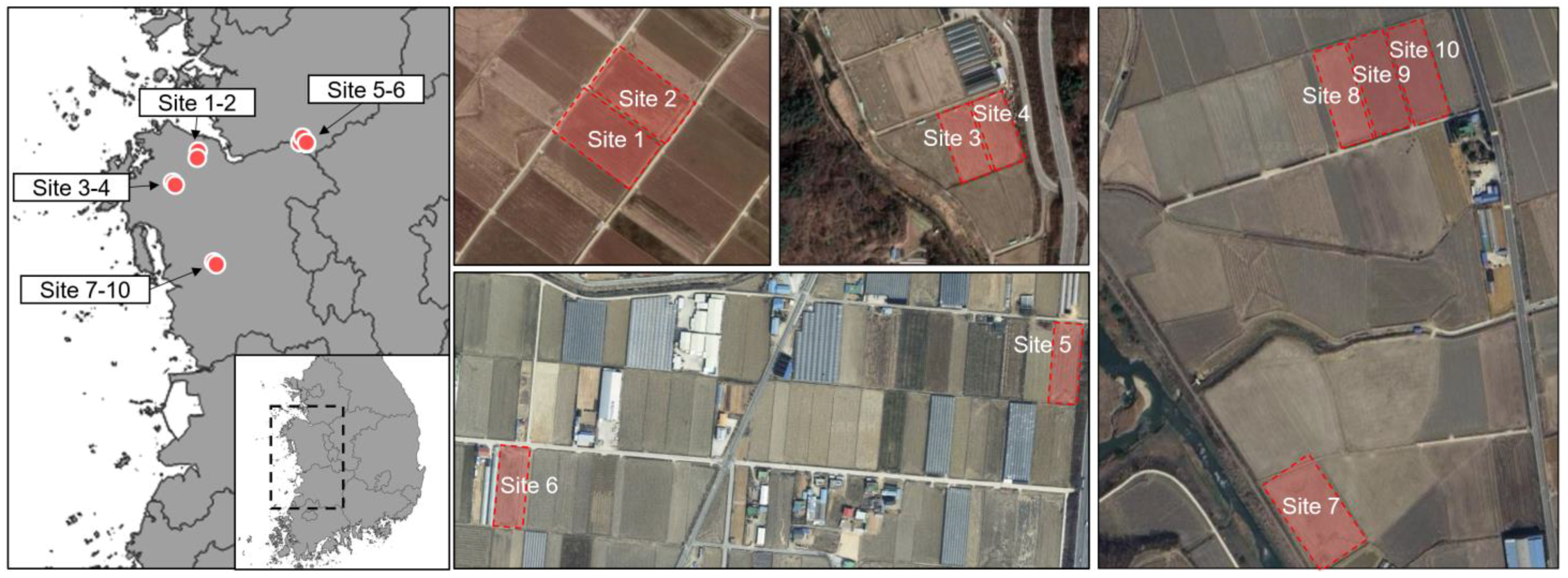
2.2.1. Field Site
2.2.2. Soil Environment Measurement
2.2.3. Field Experiment Conditions
2.3. Data Analysis
2.3.1. Load Factor Analysis
2.3.2. Correlation Analysis
2.3.3. Regression Analysis
3. Results
3.1. Soil Physical Properties
3.2. Engine Load Characteristics
3.3. Effect of Soil Physical Properties on Engine Load
4. Discussion
5. Conclusions
Author Contributions
Funding
Institutional Review Board Statement
Informed Consent Statement
Data Availability Statement
Conflicts of Interest
References
- Zhang, L.; Xu, M.; Chen, H.; Li, Y.; Chen, S. Globalization, green economy and environmental challenges: State of the art review for practical implications. Front. Environ. Sci. 2022, 10, 870271. [Google Scholar] [CrossRef]
- National Institute of Environmental Research Center (NIER). Standard Operations Procedure for the Construction of Supporting Data for National Air Pollutant Emissions; NIER: Incheon, Republic of Korea, 2019; Available online: https://www.air.go.kr/article/view.do?boardId=8&articleId=89&boardId=8&menuId=49¤tPageNo=1 (accessed on 25 September 2023).
- National Air Emission Inventory and Research Center (NAIR). Handbook of Estimation Methods for National Air Pollutant Emissions V; NAIR: Cheongju, Republic of Korea, 2022; Available online: https://www.air.go.kr/article/view.do?boardId=8&articleId=238&boardId=8&menuId=49¤tPageNo=1 (accessed on 25 September 2023).
- National Air Emission Inventory and Research Center (NAIR). 2019 National Air Pollutant Emissions; NAIR: Cheongju, Republic of Korea, 2022; Available online: https://www.air.go.kr/article/view.do?boardId=7&articleId=145&boardId=7&menuId=48¤tPageNo=1 (accessed on 25 September 2023).
- National Institute of Agricultural Sciences (NIAS). 2019 Investigation of Agricultural Machinery Usage; NIAS: Wanju, Republic of Korea, 2020. [Google Scholar]
- Kim, W.S.; Lee, S.E.; Baek, S.M.; Baek, S.Y.; Jeon, H.H.; Kim, T.J.; Lim, R.G.; Choi, J.Y.; Kim, Y.J. Evaluation of exhaust emissions factor of agricultural tractors using portable emission measurement system (PEMS). J. Drive Control 2023, 20, 15–24. [Google Scholar]
- Zhang, G.; Sandanayake, M.; Setunge, S.; Li, C.; Fang, J. Selection of emission factor standards for estimating emissions from diesel construction equipment in building construction in the Australian context. J. Environ. Manag. 2017, 187, 527–536. [Google Scholar] [CrossRef] [PubMed]
- Lee, J.H.; Jeon, H.H.; Baek, S.Y.; Baek, S.M.; Kim, W.S.; Siddique, M.A.A.; Kim, Y.J. Analysis of Emissions of Agricultural Tractor according to Engine Load Factor during Tillage Operation. J. Drive Control 2022, 19, 54–61. [Google Scholar]
- Tan, D.; Tan, J.; Peng, D.; Fu, M.; Zhang, H.; Yin, H.; Ding, Y. Study on real-world power-based emission factors from typical construction machinery. Sci. Total Environ. 2021, 799, 149436. [Google Scholar] [CrossRef] [PubMed]
- Lee, S.E.; Kim, T.J.; Kim, Y.J.; Lim, R.G.; Kim, W.S. Analysis of Engine Load Factor for Agricultural Cultivator during Plow and Rotary Tillage Operation. J. Drive Control 2023, 20, 31–39. [Google Scholar]
- Baek, S.M.; Kim, W.S.; Baek, S.Y.; Jeon, H.H.; Lee, D.H.; Kim, H.K.; Kim, Y.J. Analysis of engine load factor for a 78 kW class agricultural tractor according to agricultural operations. J. Drive Control 2022, 19, 16–25. [Google Scholar]
- Lee, D.I.; Park, J.; Shin, M.; Lee, J.; Park, S. Characteristics of Real-World Gaseous Emissions from Construction Machinery. Energies 2022, 15, 9543. [Google Scholar] [CrossRef]
- Shin, D.H.; Park, Y.S.; Yoo, C.; Park, S.H. Study on Real-Work NOx Emission Characteristics according to Load Factor of Excavator. J. Drive Control 2023, 20, 1–8. [Google Scholar]
- Barati, K.; Shen, X. Operational level emissions modelling of on-road construction equipment through field data analysis. Autom. Constr. 2016, 72, 338–346. [Google Scholar] [CrossRef]
- Koo, Y.M. PTO torque and draft analyses of an integrated tractor-mounted implement for round ridge preparation. J. Biosyst. Eng. 2022, 47, 330–343. [Google Scholar] [CrossRef]
- Kim, J.T.; Im, D.; Cho, S.J.; Park, Y.J. A Study on the Prediction of Driving Performance of Agricultural Tractors Driving on Dry Sand. J. Biosyst. Eng. 2022, 47, 502–509. [Google Scholar] [CrossRef]
- Inchebron, K.; Seyedi, S.M.; Tabatabaekoloor, R. Performance evaluation of a light tractor during plowing at different levels of depth and soil moisture content. Int. Res. J. Appl. Basic Sci. 2012, 3, 626–631. [Google Scholar]
- Kim, W.S.; Kim, Y.J.; Park, S.U.; Kim, Y.S. Influence of soil moisture content on the traction performance of a 78-kW agricultural tractor during plow tillage. Soil Tillage Res. 2021, 207, 104851. [Google Scholar] [CrossRef]
- Rasool, S.; Raheman, H. Improving the tractive performance of walking tractors using rubber tracks. Biosyst. Eng. 2018, 167, 51–62. [Google Scholar] [CrossRef]
- Battiato, A.; Diserens, E. Tractor traction performance simulation on differently textured soils and validation: A basic study to make traction and energy requirements accessible to the practice. Soil Tillage Res. 2017, 166, 18–32. [Google Scholar] [CrossRef]
- Han, G.; Kim, K.D.; Ahn, D.V.; Park, Y.J. Comparative Analysis of Tractor Ride Vibration According to Suspension System Configuration. J. Biosyst. Eng. 2023, 48, 69–78. [Google Scholar] [CrossRef]
- Choudhary, S.; Upadhyay, G.; Patel, B.; Naresh; Jain, M. Energy requirements and tillage performance under different active tillage treatments in sandy loam soil. J. Biosyst. Eng. 2021, 46, 353–364. [Google Scholar] [CrossRef]
- Ayers, P.D.; Perumpral, J.V. Moisture and density effect on cone index. Trans. ASAE 1982, 25, 1169–1172. [Google Scholar] [CrossRef]
- ASABE Standards EP542; Procedure for Using and Reporting Data Obtained with the Soil Cone Penetrometer. American Society of Agricultural and Biological Engineers: St. Joseph, MO, USA, 2019.
- Reicosky, D. Managing Soil Health for Sustainable Agriculture Volume 2: Monitoring and Management; Burleigh Dodds Science Publishing: Cambridge, UK, 2018. [Google Scholar]
- Tan, K.H. Soil Sampling, Preparation, and Analysis; CRC Press: New York, NY, USA, 1995; ISBN 0-8247-9675-6. [Google Scholar]
- Kim, W.S.; Lee, D.H.; Kim, Y.J.; Kim, Y.S.; Park, S.U. Estimation of Axle Torque for an Agricultural Tractor Using an Artificial Neural Network. Sensors 2021, 21, 1989. [Google Scholar] [CrossRef]
- Kim, W.S.; Kim, Y.J.; Baek, S.Y.; Baek, S.M.; Kim, Y.S.; Choi, Y.; Kim, Y.K.; Choi, I.S. Traction performance evaluation of a 78-kW-class agricultural tractor using cone index map in a Korean paddy field. J. Terramechanics 2020, 91, 285–296. [Google Scholar] [CrossRef]
- Chancellor, W.; Thai, N. Automatic control of tractor transmission ratio and engine speed. Trans. ASAE 1984, 27, 642–0646. [Google Scholar] [CrossRef]
- Salmerón Gómez, R.; Rodríguez Sánchez, A.; García, C.G.; García Pérez, J. The VIF and MSE in Raise Regression. Mathematics 2020, 8, 605. [Google Scholar] [CrossRef]
- Kim, Y.S.; Lee, S.D.; Baek, S.M.; Baek, S.Y.; Jeon, H.H.; Lee, J.H.; Kim, W.-S.; Shim, J.Y.; Kim, Y.J. Analysis of the effect of tillage depth on the working performance of tractor-moldboard plow system under various field environments. Sensors 2022, 22, 2750. [Google Scholar] [CrossRef]


| Item | Specifications | |
|---|---|---|
| Dimensions (length × width × height) (mm) | 4225 × 2140 × 2830 | |
| Empty weight (kg) | 3985 | |
| Engine | Make | DOOSAN INFRACORE |
| Type | In-line, 4-cycle | |
| Aspiration | Turbocharged and intercooler | |
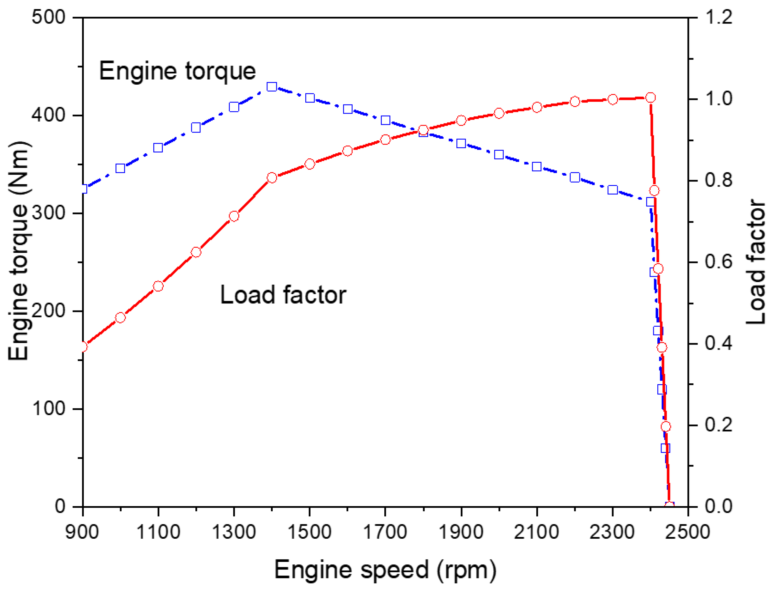
| Rated torque (Nm) | 324 @2300 rpm | |
| Rated power (kW) | 78 @2300 rpm | |
| Max. torque (Nm) | 430 @1400 rpm | |
| Torque rise (%) | 31.3 | |
| Maximum speed (rpm) | 2450 | |
| Bore × Stroke (mm) | 98 × 113 | |
| Total displacement (cc) | 3409 | |
| Compression ratio | 17:1 | |
| Dry weight (kg) | 500 | |
| Emission Compliance | TIER4-Final/EU STAGE Ⅳ | |
| Transmission | Type | Power shuttle |
| Gear stage (Forward/Reverse) | 32/32 | |
| Item | Specification |
|---|---|
| Soil moisture sensor | Measurement units: percentage of volumetric water content (VWC) Range: 0% VWC to saturation Accuracy: ±3.0% VWC |
| Cone penetrometer | Measurement units: cone index (kPa) Range: 0 to 45 cm, 0 to 7000 kPa Accuracy: ±1.25 cm, ±103 kPa |
| Sites | Field Size (m) | Location | Latitude | Longitude | Experimental Year |
|---|---|---|---|---|---|
| 1 | 60 × 100 | Seosan | 36°46′44.4″ N | 126°33′27.0″ E | 2017 |
| 2 | 60 × 100 | Seosan | 36°46′46.2″ N | 126°33′28.8″ E | 2017 |
| 3 | 40 × 100 | Cheongyang | 36°30′35.3″ N | 126°47′27.5″ E | 2017 |
| 4 | 40 × 100 | Cheongyang | 36°30′35.9″ N | 126°47′29.1″ E | 2017 |
| 5 | 30 × 100 | Anseong | 36°56′42.7″ N | 127°14′33.2″ E | 2019 |
| 6 | 40 × 100 | Anseong | 36°56′37.8″ N | 127°14′04.5″ E | 2019 |
| 7 | 60 × 100 | Dangjin | 36°55′50.0″ N | 126°37′57.5″ E | 2019 |
| 8 | 40 × 100 | Dangjin | 36°56′04.1″ N | 126°37′58.3″ E | 2019 |
| 9 | 40 × 100 | Dangjin | 36°56′04.3″ N | 126°37′59.8″ E | 2019 |
| 10 | 40 × 100 | Dangjin | 36°56′04.8″ N | 126°38′01.5″ E | 2019 |
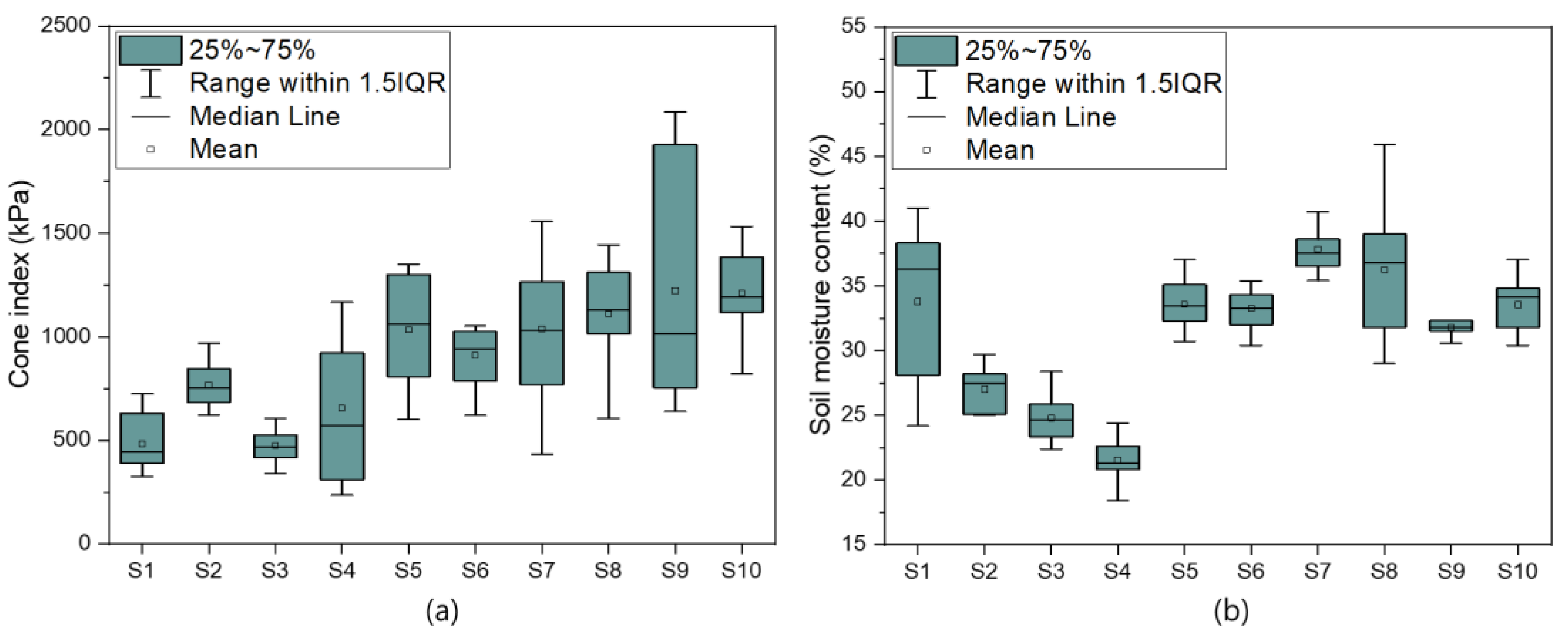
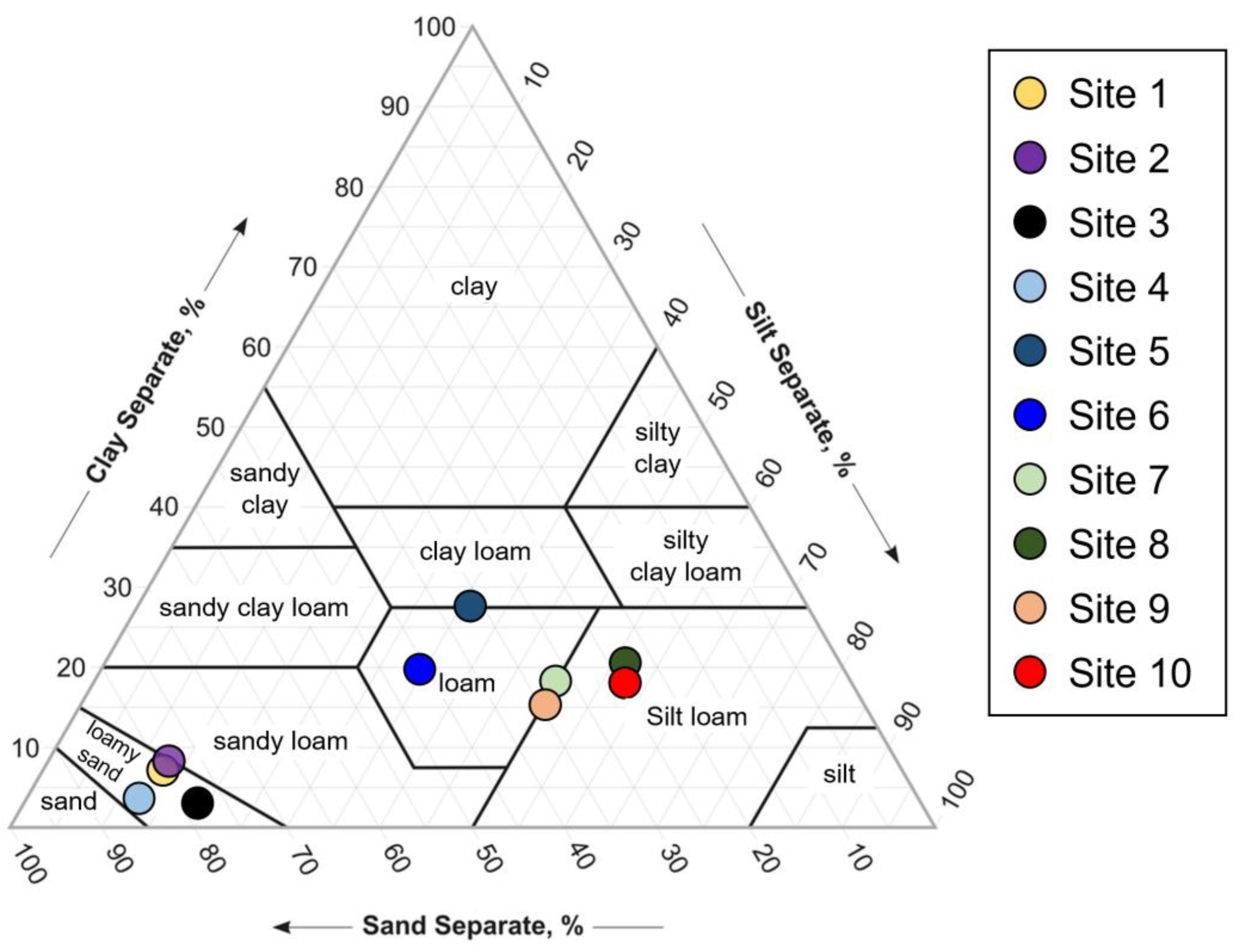
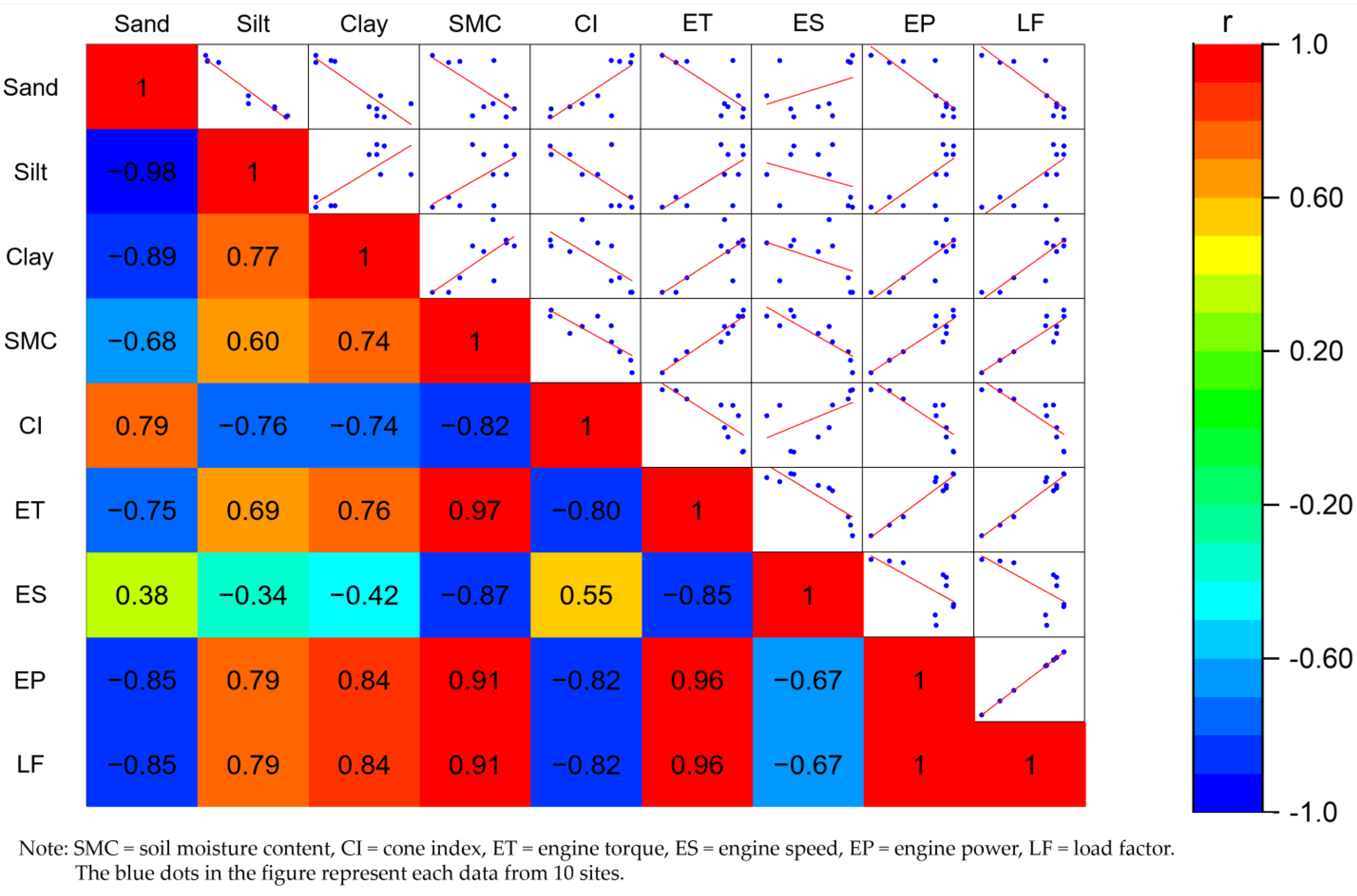
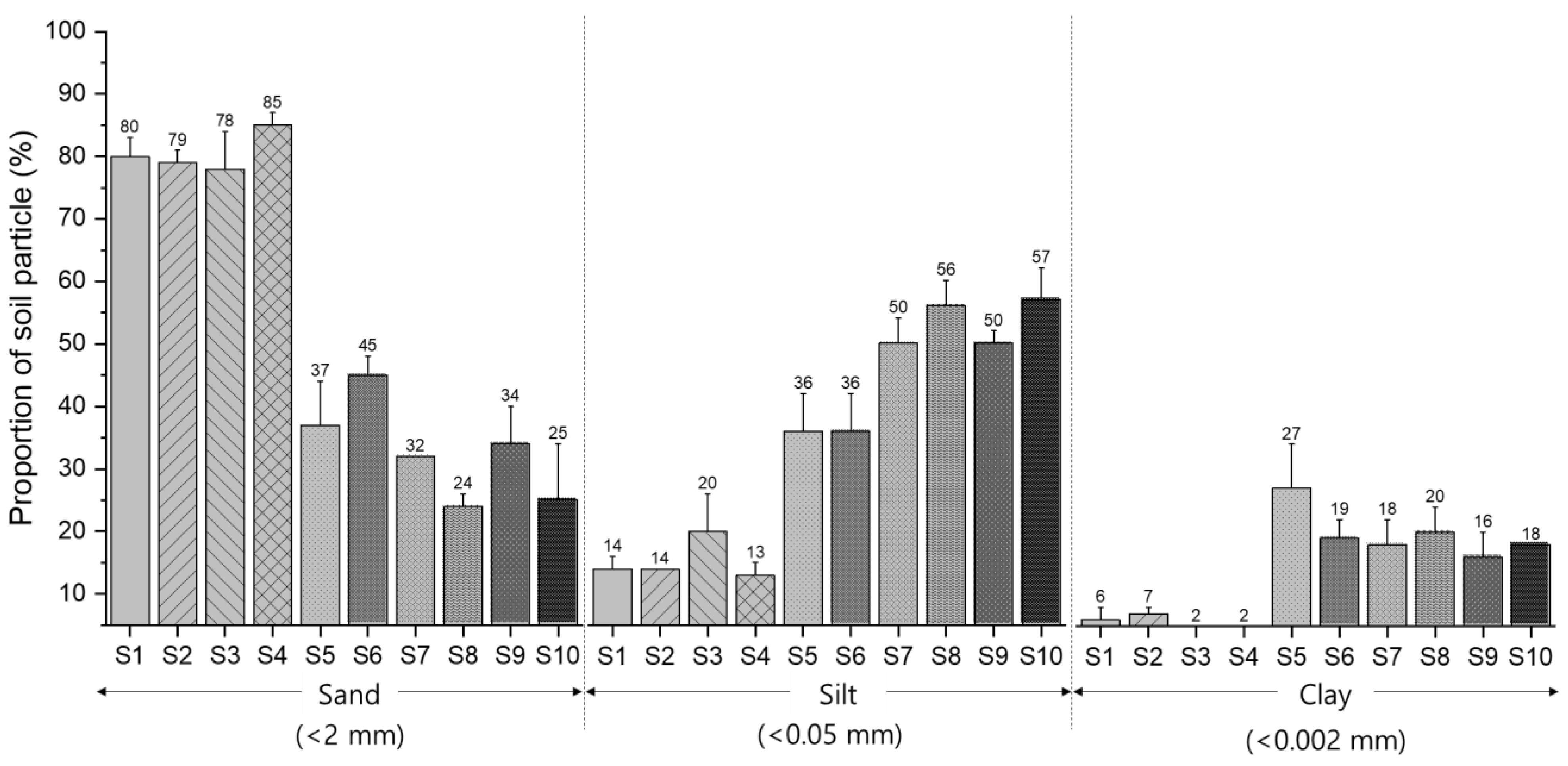
| Sites | SMC (%) | CI (kPa) | Soil Particle Proportions (%) | Soil Texture | ||
|---|---|---|---|---|---|---|
| Sand (<2 mm) | Silt (<0.05 mm) | Clay (<0.002 mm) | ||||
| 1 | 33.79 b,c | 483 e | 80.00 b | 14.00 e | 6.00 d | Loamy sand |
| 2 | 27.01 d | 768 c,d | 79.00 b | 14.00 e | 7.00 d | Loamy sand |
| 3 | 24.79 d | 476 e | 78.00 b | 20.00 d | 2.00 e | Loamy sand |
| 4 | 21.55 e | 656 d,e | 85.00 a | 13.00 e | 2.00 e | Loamy sand |
| 5 | 33.60 b,c | 1034 a,b,c | 37.00 d | 36.00 c | 27.00 a | Clay loam |
| 6 | 33.27 c | 910 b,c,d | 45.00 c | 36.00 c | 19.00 b | Loam |
| 7 | 37.84 a | 1038 a,b,c | 32.00 e | 50.00 b | 18.00 b,c | Loam |
| 8 | 36.24 a,b | 1111 a,b | 24.00 f | 56.00 a | 20.00 b | Silt loam |
| 9 | 31.77 c | 1223 a | 34.00 e | 50.00 b | 16.00 c | Silt loam |
| 10 | 33.54 b,c | 1212 a | 25.00 f | 57.00 a | 18.00 b,c | Silt loam |
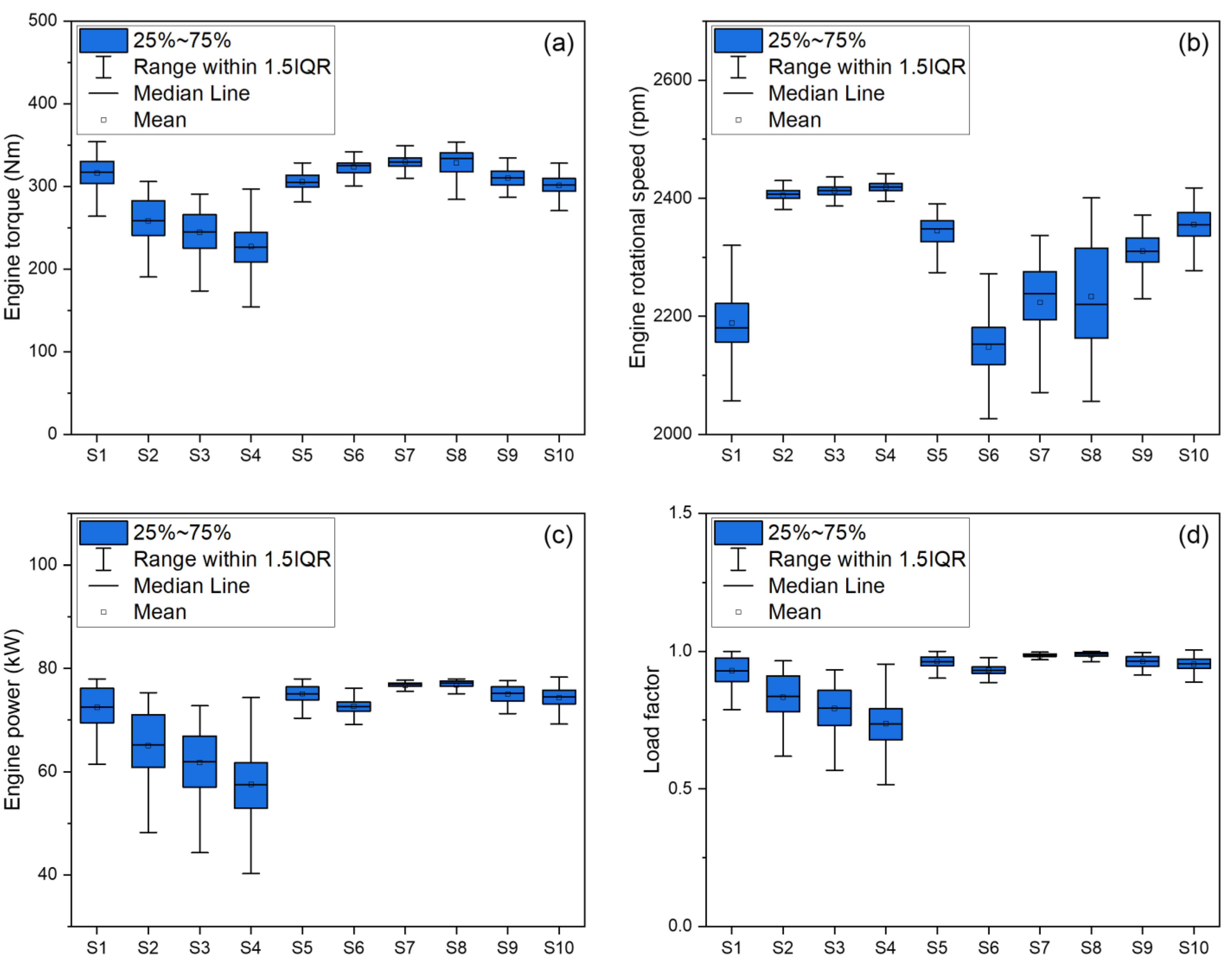
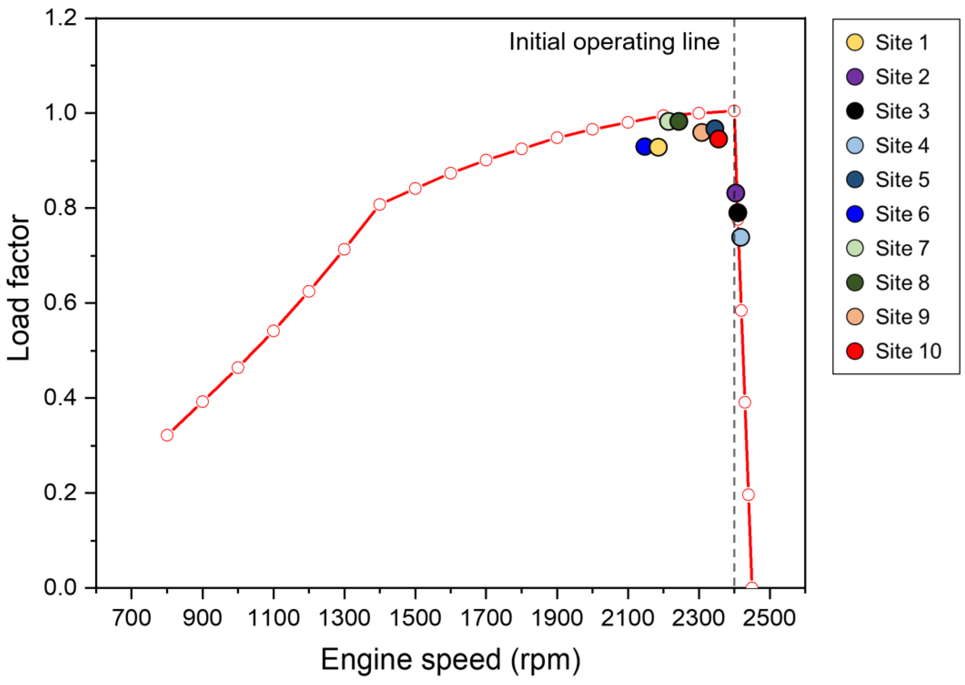
| Sites | Engine Rotational Speed (rpm) | Engine Torque (Nm) | Engine Power (kW) | Load Factor |
|---|---|---|---|---|
| 1 | 2189 i | 316.4 d | 72.47 e | 0.929 e |
| 2 | 2405 c | 258.3 h | 65.03 f | 0.834 f |
| 3 | 2413 b | 244.6 i | 61.77 g | 0.792 g |
| 4 | 2419 a | 227.2 j | 57.52 h | 0.737 h |
| 5 | 2345 e | 305.8 f | 75.07 b | 0.962 b |
| 6 | 2148 j | 323.4 c | 72.70 d | 0.932 d |
| 7 | 2224 h | 329.7 a | 76.71 a | 0.983 a |
| 8 | 2233 g | 328.8 b | 76.76 a | 0.984 a |
| 9 | 2310 f | 310.3 e | 75.05 b | 0.962 b |
| 10 | 2356 d | 301.4 g | 74.32 c | 0.953 c |
| Model | Source | Regression Model | R2 | R2 Adj | S.E. |
|---|---|---|---|---|---|
| A | = 0.0147 + 0.4487 | 0.824 | 0.803 | 0.0388 | |
| B | = −0.000255 + 1.1343 | 0.678 | 0.638 | 0.0525 | |
| C | = −0.00292 + 1.0582 | 0.718 | 0.683 | 0.0491 | |
| D | = 0.0114 − 0.000076 + 0.6168 | 0.844 | 0.800 | 0.0391 | |
| E | = 0.00997 − 0.00147 + 0.6719 | 0.924 | 0.902 | 0.0274 | |
| F | LF = −0.000126 − 0.001804 + 1.1130 | 0.780 | 0.717 | 0.0465 | |
| G | = 0.0108SMC + 0.000030 − 0.00162Sp + 0.6282 | 0.926 | 0.888 | 0.0291 |
| Model | Degrees of Freedom (Df) | Sum of Squares (SS) | Mean Squares (MS) | F-Value | p-Value | Variable | Tolerance | Variance Inflation Factor (VIF) | |
|---|---|---|---|---|---|---|---|---|---|
| A | Regression | 1 | 0.0565 | 0.0565 | 37.381 | 0.000 * | SMC | ||
| Residual | 8 | 0.0120 | 0.0015 | ||||||
| B | Regression | 1 | 0.0464 | 0.0464 | 16.848 | 0.003 * | CI | ||
| Residual | 8 | 0.0221 | 0.0028 | ||||||
| C | Regression | 1 | 0.0492 | 0.0492 | 20.370 | 0.002 * | Sand | ||
| Residual | 8 | 0.0193 | 0.0024 | ||||||
| D | Regression | 2 | 0.0578 | 0.0289 | 18.964 | 0.001 * | SMC | 0.331 | 3.201 |
| Residual | 7 | 0.0107 | 0.0015 | CI | 0.331 | 3.201 | |||
| E | Regression | 2 | 0.0633 | 0.0316 | 42.278 | 0.000 * | SMC | 0.539 | 1.854 |
| Residual | 7 | 0.0052 | 0.0007 | Sand | 0.539 | 1.854 | |||
| F | Regression | 2 | 0.0534 | 0.0267 | 12.375 | 0.005 * | CI | 0.370 | 2.703 |
| Residual | 7 | 0.0151 | 0.0022 | Sand | 0.370 | 2.703 | |||
| G | Regression | 3 | 0.0634 | 0.0211 | 24.881 | 0.001 * | SMC | 0.329 | 3.042 |
| Residual | 6 | 0.0051 | 0.0008 | CI | 0.225 | 4.435 | |||
| Sand | 0.367 | 2.722 | |||||||
| Site | SMC (%) | CI (kPa) | Soil Texture | LF | ||
|---|---|---|---|---|---|---|
| Sand (%) | Silt (%) | Clay (%) | ||||
| 1 | 19.45 | 689.69 | 68 | 20 | 21 | 0.793 |
| 2 | 24.50 | 563.21 | 40 | 48 | 12 | 0.852 |
| 3 | 20.24 | 864.67 | 40 | 28 | 32 | 0.921 |
| Items | Model A | Model B | Model C | Model D | Model E | Model F | Model G | |
|---|---|---|---|---|---|---|---|---|
| Site 1 | Average LF (Kim et al. [31]) | 0.793 | ||||||
| Estimated LF | 0.734 | 0.956 | 0.860 | 0.787 | 0.766 | 0.902 | 0.748 | |
| Error (%) | 7.43 | 20.58 | 8.47 | 0.80 | 3.44 | 13.79 | 5.64 | |
| Site 2 | Average LF (Kim et al. [31]) | 0.852 | ||||||
| Estimated LF | 0.808 | 0.991 | 0.942 | 0.855 | 0.857 | 0.970 | 0.844 | |
| Error (%) | 5.20 | 16.21 | 10.47 | 0.26 | 0.57 | 13.77 | 1.00 | |
| Site 3 | Average LF (Kim et al. [31]) | 0.921 | ||||||
| Estimated LF | 0.746 | 0.914 | 0.942 | 0.783 | 0.815 | 0.932 | 0.807 | |
| Error (%) | 19.09 | 0.84 | 2.19 | 15.02 | 11.58 | 1.11 | 12.43 | |
| Average | MAPE (%) | 10.57 | 12.55 | 7.04 | 5.36 | 5.19 | 9.56 | 6.35 |
| RMSE | 0.110 | 0.124 | 0.065 | 0.080 | 0.064 | 0.093 | 0.071 | |
| RD (%) | 12.87 | 14.44 | 7.66 | 9.35 | 7.44 | 10.85 | 8.31 | |
Disclaimer/Publisher’s Note: The statements, opinions and data contained in all publications are solely those of the individual author(s) and contributor(s) and not of MDPI and/or the editor(s). MDPI and/or the editor(s) disclaim responsibility for any injury to people or property resulting from any ideas, methods, instructions or products referred to in the content. |
© 2023 by the authors. Licensee MDPI, Basel, Switzerland. This article is an open access article distributed under the terms and conditions of the Creative Commons Attribution (CC BY) license (https://creativecommons.org/licenses/by/4.0/).
Share and Cite
Min, Y.-S.; Kim, Y.-S.; Lim, R.-G.; Kim, T.-J.; Kim, Y.-J.; Kim, W.-S. The Influence of Soil Physical Properties on the Load Factor for Agricultural Tractors in Different Paddy Fields. Agriculture 2023, 13, 2073. https://doi.org/10.3390/agriculture13112073
Min Y-S, Kim Y-S, Lim R-G, Kim T-J, Kim Y-J, Kim W-S. The Influence of Soil Physical Properties on the Load Factor for Agricultural Tractors in Different Paddy Fields. Agriculture. 2023; 13(11):2073. https://doi.org/10.3390/agriculture13112073
Chicago/Turabian StyleMin, Yi-Seo, Yeon-Soo Kim, Ryu-Gap Lim, Taek-Jin Kim, Yong-Joo Kim, and Wan-Soo Kim. 2023. "The Influence of Soil Physical Properties on the Load Factor for Agricultural Tractors in Different Paddy Fields" Agriculture 13, no. 11: 2073. https://doi.org/10.3390/agriculture13112073
APA StyleMin, Y.-S., Kim, Y.-S., Lim, R.-G., Kim, T.-J., Kim, Y.-J., & Kim, W.-S. (2023). The Influence of Soil Physical Properties on the Load Factor for Agricultural Tractors in Different Paddy Fields. Agriculture, 13(11), 2073. https://doi.org/10.3390/agriculture13112073