A Gas Diffusion Analysis Method for Simulating Surface Nitrous Oxide Emissions in Soil Gas Concentrations Measurement

Abstract

The detection of low gas concentrations from the soil surface demands expensive high-precision devices to estimate nitrous oxide (N₂O) flux. As the prevalence of N₂O concentration in the soil atmosphere is higher than its surface, the present study aimed to simulate N₂O surface flux (CF) from soil gas measured in a soil-interred silicone diffusion cell using a low-cost device. The methodological steps included the determination of the diffusion coefficient of silicone membrane (D_slcn), the measurement of the temporal variations in the N₂O gas in the soil (C_si) and on the surface (MF), and the development of a simulation process for predicting CF. Two experiments varying the procedure and periods of soil moisture saturation in each fertilized soil sample were conducted to detect C_si and MF. Using D_slcn and C_si, the variations in the soil gas (C_soil) were predicted by solving the diffusion equation using the implicit finite difference analysis method. Similarly, using six soil gas diffusivity models, the CF values were simulated from C_soil. For both experiments, statistical tests confirmed the good agreement of CF with MF for soil gas diffusivity models 4 and 5. We suggest that the tested simulation method is appropriate for predicting N₂O surface emissions.

1. Introduction

Accelerated crop production ensures food security for the global population. High-yielding crop varieties that consume significant amounts of synthetic fertilizers are being cultivated to secure food production needs [1]. Nitrogen-based fertilizers are essential for plants during their growth stages [2]. In addition to synthetic fertilizers, the use of organic manure in the forms of crop residues, animal waste, and biological N-fixing plants is common in plant nutrient supply chains [3,4]. By 2019, the global average atmospheric nitrous oxide (N₂O) concentration had increased to 333.2 ppbv [5]. The use of synthetic fertilizers is one of the major causes of these changes [6]. The contribution of N₂O to atmospheric warming is 298 times greater than that of carbon dioxide, and it significantly contributes to the depletion of the stratospheric ozone layer [7,8]. Therefore, control of fertilizer application levels is highly needed to limit the N₂O emissions from the crop fields. Soil can be considered as a large bioreactor that produces various materials as output [9,10], especially greenhouse gases (GHGs) [11]. Among the GHGs, methane (CH₄), carbon dioxide (CO₂), and nitrous oxide (N₂O), the nitrogen-based fertilizers highly contribute to the N₂O production via the microbial denitrification and nitrification processes in the soil [12]. The results of various experiments convey the impact of environmental and agronomic factors on the N₂O emissions from uplands [13,14,15,16]. Globally, collective strategies are being implemented to achieve the sustainable development goals (SDGs) by 2030 [17]. The assessment of N₂O emissions is vital for implementing climate-responsive actions, such as control measures to limit GHG emissions from cropping fields, controlling the use of synthetic fertilizers, and testing alternative soil nutrient enrichment methods.

According to Denmead 2008, the main techniques that are used for measuring methane and nitrous oxide fluxes in inland ecosystems and atmospheres are known as enclosure-based and micrometeorological measurements [18]. Butterbach-Bahl et al. have mentioned that the selection of the appropriate technique is mainly based on investment capacity, the demand for the findings, and the type of research question to be analyzed [19]. As mentioned in the work of Maljanen et al. [20], the chamber technique is commonly used to estimate N₂O fluxes [21,22,23]. According to Butterbach-Bahl et al., homogenous fields, including those with trees, slopes, and that are building-free, and the mono-crop condition are required for micrometeorological measurements, and the related measurement instruments should be high-precision fast-response devices. When using this technique, the expense for conducting the onsite measurement in one station has been indicated to be USD 60,000–80,000 for CO₂, and this price can be increased by USD 30,000 to USD 40,000 for each additional gas (CH₄, N₂O, etc.) if needed. In 2014, Chikowo et al. also mentioned the inappropriateness of micrometeorological techniques in small-scale farming systems that insist on intercropping, a soil fertility gradient, and complicated land use patterns [24]. The chamber method can be identified as a system that directly samples gas from the soil surface through the use of permanently installed enclosed chambers. In the chamber method, suites for small-scale cultivated areas are created by establishing small, simple chambers on the soil surface. The chamber method can operate manually or automatically when taking gas samples for gas monitoring [19,25]. Since gas sampling is performed within the chamber, a small area of the field is represented when calculating the emissions, and the installation of the chamber disturbs the natural environmental conditions of the soil gas diffusion process. According to the air circulation schedule, there are two types of chambers called static and dynamic chambers, in which the chamber gas is replaced rapidly while measurements continue and while scheduled ventilation takes place after the gas has been collected in the chamber for a period of time [26,27]. Low-level N₂O gas concentrations are more prevalent in the chamber than in the soil atmosphere, since gas diffuses from the soil surface to the atmosphere. Therefore, chamber methods also require high-precision gas-monitoring devices and related accessories, increasing the measurement cost. Conversely, the operating costs of the gas-monitoring process limit the expansion of estimation activities for GHG emissions. It is necessary to develop techniques that use low-cost gas-monitoring devices together with an accurate gas-sampling system to better estimate N₂O gas emissions.

Compared to surface emissions, a higher N₂O gas concertation level is prevalent in the soil atmosphere [28]. This supports the development of a low-cost gas-monitoring instrument to measure the N₂O gas releasing activities in the soil atmosphere if gas samples are collected effectively. The soil gas sampling can be carried out indirectly by inserting a perforated pipe or silicone tube into the soil, and the process is known as the passive gas sampling method. The soil gas then surrounds the tube and equilibria with the inner gas level via a gas diffusion process [29,30,31]. Because of its molecular structure, silicone has special characteristics that make it suitable for soil gas sampling, such as water repellence, releasability, cold resistance, and high gas diffusivity. In various studies, these silicone tubes have been tested to determine their gas sampling ability [32,33,34]. The results of previous studies have demonstrated the suitability of silicone tubes [35] and perforated stainless-steel pipes [36] for soil gas sampling in continuous automated sampling methods and manual sampling methods. Nondispersive infrared (NDIR) technology has been successfully applied to develop GHG monitoring devices for CO₂, CH₄ [37,38,39,40], and N₂O [28]. In the upper-level detection limits (upper ppm levels) shown by low-cost devices compared to high-precision devices (QCL, CRL laser-based, photoacoustic, and FTIR devices), where the detection limit shows the sub-ppm level, higher soil gas levels are more prevalent, meaning that low-cost devices can be used for gas measurements with soil gas diffusion cells.

In the process of numerical solving of soil gas flux, the gradient method has gained the most attention. In porous soil, gas flux can be estimated based on the measured gas concentrations at each level of the soil profile and the gas diffusivity of the soil by assuming that gas diffusion is the dominant gas transport mechanism in the soil [41]. Since there are high levels of uncertainty when testing the soil gas diffusivity, some research works used soil gas diffusivity model-based approximation approaches. Since flux is more sensitive when its own calculation steps are used, the use of implicit assumptions was suggested [31,42,43]. Therefore, the soil gas diffusivity model-based implicit finite difference simulation method can be used to effectively estimate the N₂O flux from measured soil gas levels.

In summary, N₂O flux assessment activities in the agricultural fields need to be accelerated to control GHG emissions. The operational costs induced by high-precision gas-monitoring devices and the related accessories that are necessary for existing gas-monitoring methodologies are major barriers to achieving the targeted gas emission estimations. Mutually, low-cost N₂O gas-monitoring devices use passive sampling methods to sample the gases in the soil (where there are higher gas levels than on the surface), and numerical simulation approaches can be used to predict gas fluxes in cost-efficient ways. Therefore, this study demonstrated a simulation approach for estimating N₂O flux on the soil surface according to the soil gas concentration measured using a low-cost measuring device connected to a silicone soil gas sampler.

2. Materials and Methods

The conceptual framework of the experiment was mainly based on the soil N₂O flux simulation process of the recorded soil N₂O levels determined by a low-cost NDIR device with a diffusion cell (silicone tube) entombed in the soil region, where there are higher gas concentration levels than in the atmosphere (Figure 1). Together with the diffusion coefficient, the inner N₂O gas concentration of the diffusion cell changes, along with the temporal variations in the soil gas concentration. From the gas concentrations recorded in the silicone diffusion cell, the predicted values on temporal changes in the soil N₂O gas concentration, hereafter C_soil, were simulated by solving the diffusion equation (Equation (4)) using the implicit finite difference method.

Secondly, the values calculated for N₂O flux on the soil surface (CF) were simulated by solving the diffusion equation (implicit finite difference method) using the six soil gas diffusivity models. To compare the simulated values, the observed surface flux of N₂O gas (MF) was calculated from monitored soil surface emission levels using a high-resolution gas-monitoring device followed by the chamber method. Accordingly, the overall experiment was based on three main steps: (1) the determination of the diffusion coefficient of the silicone membrane; (2) the measurement of the concurrent N₂O gas concentrations in the soil gas and soil surface; and (3) the development of a simulation process to determine the CF values. The simulation process is described below.

2.1. Determination of the Diffusion Coefficient of the Silicone Membrane

The observed N₂O concentration in the silicone diffusion cell was the result of the diffused soil gas travelling through the wall of the silicone tube. Therefore, the N₂O concentration in soil gas should be estimated by solving the diffusion equation according to the observed N₂O concentration in the silicone tube. The diffusion coefficient of the silicone membrane (D_slcn) was determined, since it was required to solve the diffusion equation during the simulation process. In the experimental setup, two silicone tubes (length 59 cm, internal diameter 6 mm, and external diameter 8 mm for each) were placed in an enclosed chamber (8000 mL), and the two edges of each tube were serially connected with an air circulation pump, FTIR device (system 1; Perkin Elmer—Spectrum Two FT-IR spectrometer with a long path gas cell system, 7 m optical path length, volume 500 mL, Infrared Analysis, Inc., Anaheim, USA, model 7.2-V), and a new NDIR device [28] (system 2; volume 320.3 mL) to create two separate diffused gas measurement systems (Figure 2). After adding a known N₂O gas (purity level 99.5%) volume (50 mL) into the gas chamber, the accumulated gas level in the silicone tube was measured by each device at 30-min intervals for 12 h. From the data recorded by each device, the gas concentration in the silicone tubes (system1 and system 2) and the balanced gas concentration in the gas chamber were approximately determined at each successive period by applying the difference equations below. The gas concentrations of system 1 and system 2 were calculated by solving Equation (3), and D_slcn was optimized using an R package.

$$q_1=D_s\frac{C_c-C_1}{\Delta x}A=V_1\frac{C_1-C_1^o}{\Delta t}$$

(1)

$$q_2=D_s\frac{C_c-C_2}{\Delta x}A=V_2\frac{C_2-C_2^o}{\Delta t}$$

(2)

$$V_c\frac{C_c-C_c^o}{\Delta t}=-\left(q_1+q_2\right)$$

(3)

$q_1$: rate of the diffused gas volume from container to system 1 (10⁻⁶ cm³ s⁻¹); $q_2$: rate of the diffused gas volume from container to system 2 (10⁻⁶ cm³ s⁻¹); $D_s$: gas diffusion rate in silicone membrane (cm² s⁻¹); $C_c$: gas concentration in the container (10⁻⁶ cm³/cm³); $C_1$: gas concentration in system 1 (10⁻⁶ cm³/cm³); $C_2$: gas concentration in system 2 (10⁻⁶ cm³/cm³); $C_c^o$: gas concentration of previous time step in the container (10⁻⁶ cm³/cm³); $C_1^o$ gas concentration of previous time step in system 1 (10⁻⁶ cm³/cm³); $C_2^o$: gas concentration of previous time step in system 2 (10⁻⁶ cm³/cm³); V_c: volume of the container (cm³); V₁: volume of system 1 (cm³); V₂: volume of system 2 (cm³); ∆x: thickness of the silicone tube (cm); ∆t: time step (s); A: surface area of the silicone tube (cm²).

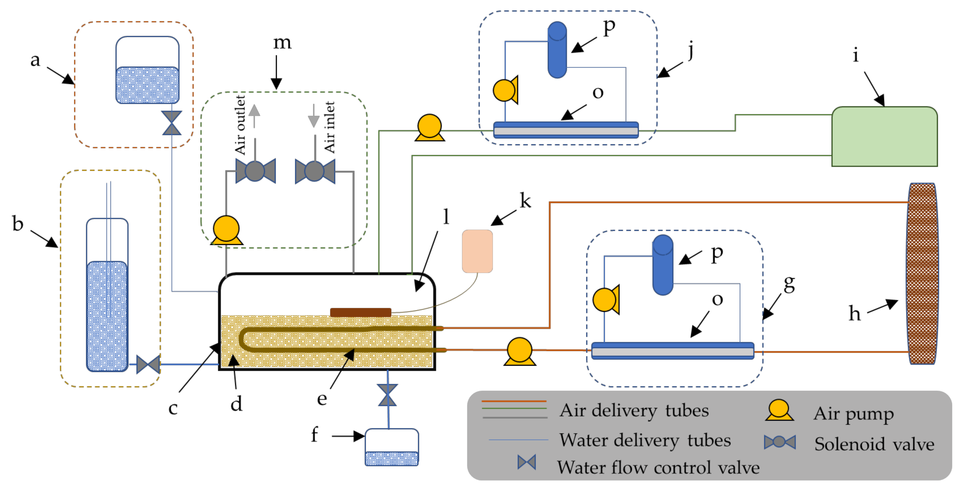
2.2. The Experimental Setup for Monitoring the N₂O Flux and Soil Atmospheric N₂O Gas Concentrations

To simulate the surface flux (CF) and compare it with the measured flux (MF), temporal variation in the soil and atmospheric N₂O concentrations should be monitored. Therefore, a laboratory test was conducted to monitor the gas concentrations in both regions (Figure 3). A soil sample (shimajiry maji) weight of 4 kg taken from the research field of the University of the Ryukyus was sieved with a 2 mm sieve (particle density: 2.685 g/cm³, bulk density: 0.958 g/cm³) and was repacked in the testing chamber (c). As an ammonium-based nitrogen source, 3 g of (NH₄)₂SO₄ was mixed with the soil. As shown in Figure 3, the experimental setup mainly consisted of serially interconnected air-drying sections (g,i) in each gas-monitoring device (h,i) to monitor the gas concentrations in the soil and atmospheric regions. The soil chamber (c) had a hole underneath and was connected to the water drainage system (f) to ensure drainage after the completion of the saturation events. There were two water supply systems that were used in the soil saturation events: the top water supply system (a) applied water to the top surface of the soil, and the bottom water supply unit (Mariotte cell) (b) provided a controlled water supply from the bottom side of the soil layer.

A silicone tube diffusion cell (length: 59 cm, internal diameter: 0.6 cm, and wall thickness: 0.1 mm) (e) was buried in the soil 3.5 cm from the top so that the diffused soil N₂O gas could accumulate into it through the wall, and the two ends of the tube were serially connected with a low-cost gas-monitoring device (h). Data were recorded in 30-min intervals. The diffused air was circulated within the system using an air pump (AS ONE-EAP-01). The circulated air was sent through a drying section to avoid water accumulation in the system when it was operating over long periods of time. The drying sections were developed by using membrane-type dryers (Suncep SWG-A01-03) (o) consisting of two eccentric tubes. The outward tube for dry gas circulation was connected to a silicone moisture absorber (p), and the middle tube was for soil gas circulation.

To monitor the headspace gas levels, an FTIR spectrometer (i) was used. The measurement schedule for the headspace gas was every 1 min over a 30-min period in a closed chamber and over 1 h of chamber ventilation (by ventilation system (m)) period. The gas flux was calculated from the slope according to the gas concentration in the last seven minutes during the closed-chamber period. A sensor connected to a data logger (moisture meter embedded with a thermometer) (k) was placed in the soil container, and data were recorded at 30-min intervals.

To test the gas diffusion at different volumetric water levels, the water supply and drainage events were carried out under different conditions for each experiment. Using the different water supply methods, two experiments were conducted in which saturation took place over different periods of time. The first experiment was based on the bottom-side water supply, in which a Mariotte cell (b) was used to control the water supply drop by drop. The saturation and drainage periods were both two days long. During the saturation period, the bottom edge of the Mariotte cell’s air intake tube was maintained at the same level as the soil in the chamber. In the second experiment, the top-side water supply unit (a) was used to control the water supply (rate: 0.05 mL S⁻¹) over a two-day saturation period, and the soil was allowed to drain with the help of gravity over the course of three days. The drainage steps in each experiment included open gravity drainage (experiment 1) and flow-controlled gravity drainage (rate: 0.05 mL S⁻¹) (experiment 2). For both experiments, concurrent soil gas concentration was measured by each device according to the abovementioned measurement schedules.

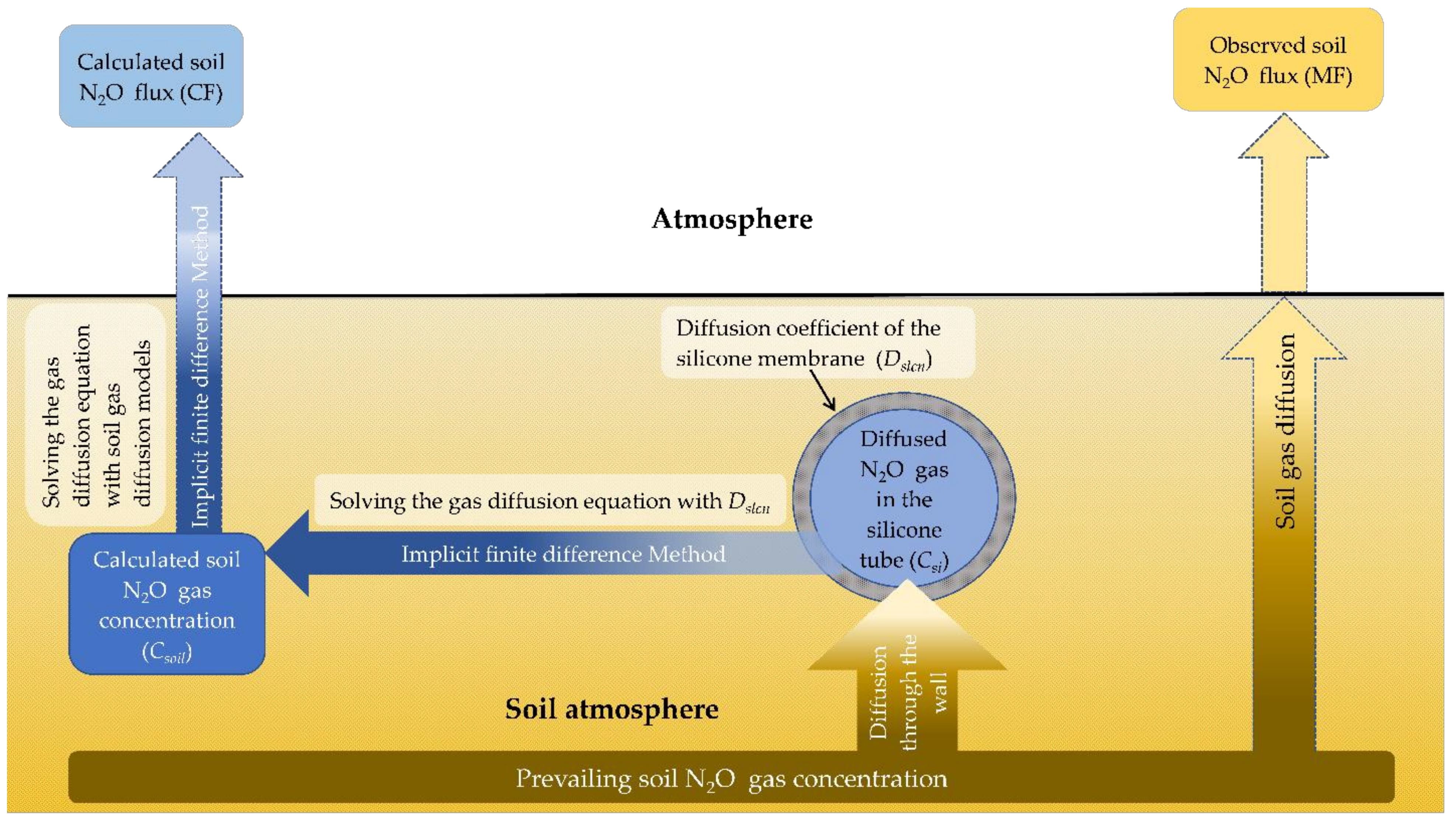
2.3. Simulation Steps for Predicted N₂O Surface Flux (CF)

The two simulation steps were followed as indicated in Figure 1. The first step was to simulate C_soil according to the measured gas concentrations in a silicone diffusion cell (C_si). The second step was to estimate the values for the predicted N₂O flux from the soil surface (CF). In the second step, the parameters of the soil diffusivity models were optimized on a trial-and-error basis until the CF values fit with the measured N₂O flux (MF) from the soil surface.

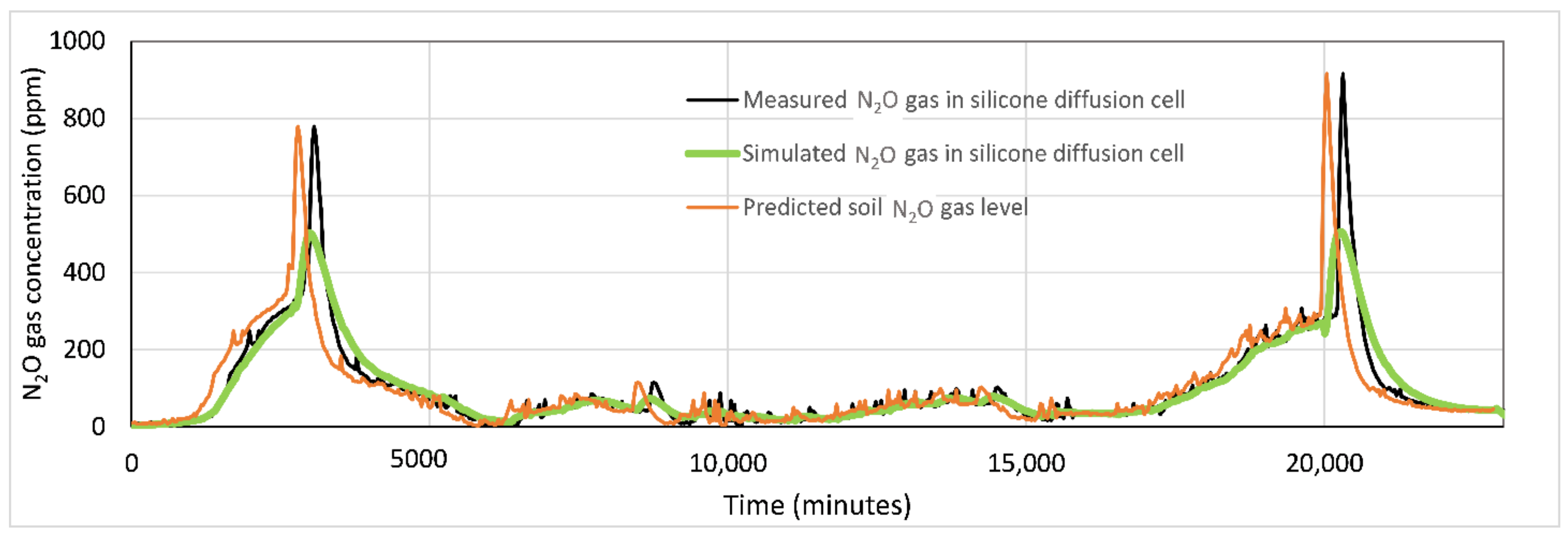
2.3.1. Simulation Steps for Predicting the Soil N₂O Gas Level from the Measured Gas in Silicone Diffusion Cell

Theoretically, the soil N₂O gas can be estimated from the inverse analysis of the diffusion equation on C_si. However, the results of the calculation did not converge satisfactorily. Therefore, we estimated the concentration of the N₂O gas in the soil (C_soil) according to the following steps: (1) C_soil was assumed to be the boundary condition of the soil side for solving the diffusion equation (Equation (4)). In the first equation, the observed C_si was used by shifting the assumed C_soil a few hours forward. For the first calculation, the observed C_si was shifted the same number of hours forward as the assumed C_soil. (2) The assumed C_soil was used to simulate the gas concentration in the silicone tube (C_ssi) by solving the diffusion equation according to the implicit finite difference method. (3) The simulated values of the C_ssi time series were compared with those of the C_si. Steps 1 to 4 were repeated until the C_ssi matched the C_si on a trial-and-error basis (Figure 4). An assumption was made about the completion of the gas measurements soon after the gas mixture entered the silicone diffusion cell.

$$\frac{\partial C_{si}}{\partial t}=D_{slcn}\frac{{\partial }^2{C}_{si}}{\partial x^2}$$

(4)

where:

$C_{si}$: N₂O concentration in the silicone diffusion cell (g gas m⁻³ diffusion cell air);

$D_{slcn}$: gas diffusion coefficient of the silicone membrane (m³ gas m⁻¹ silicone s⁻¹);

∆x: thickness of the silicone tube (m); ∆t: time step (s).

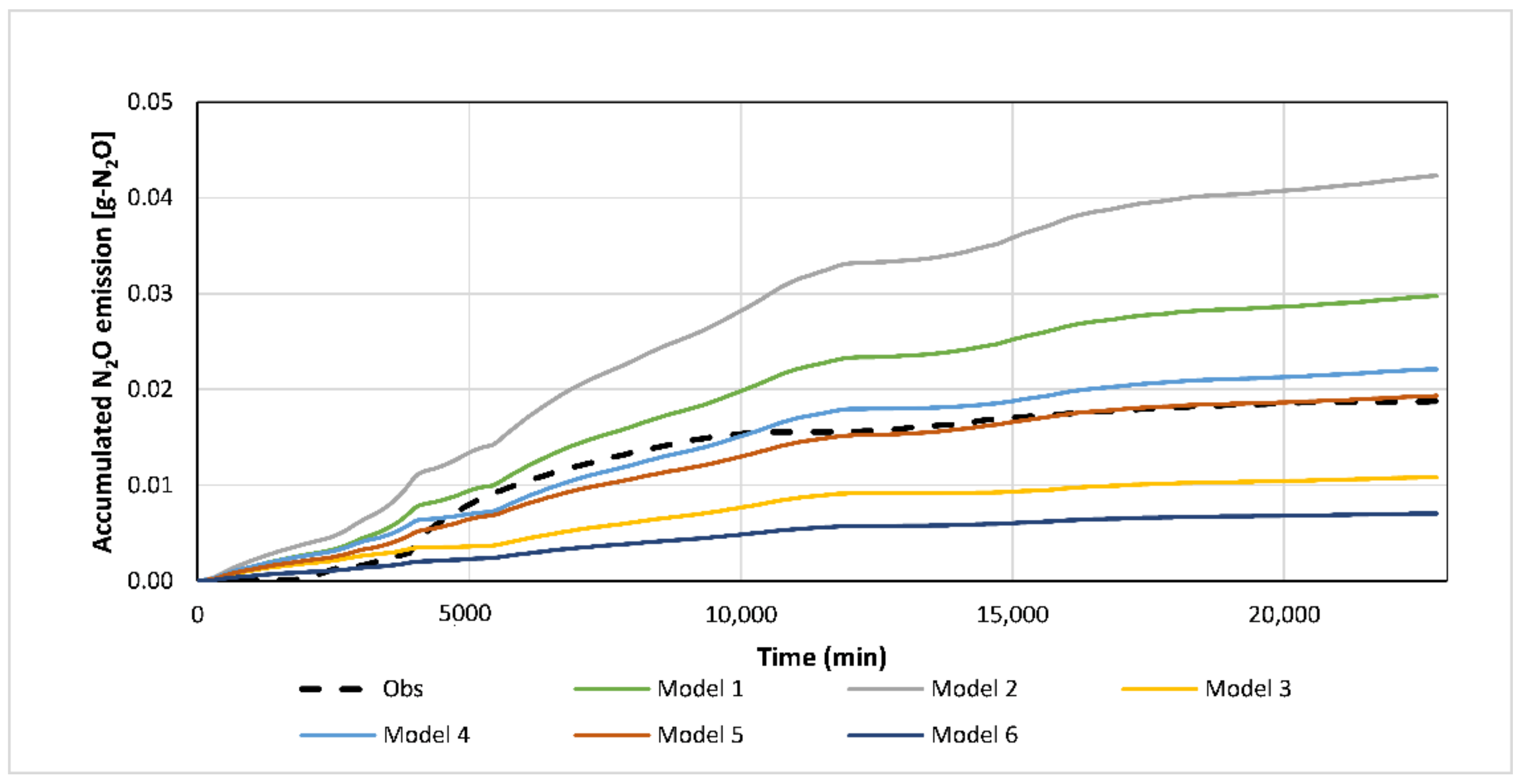
2.3.2. Steps for Simulating the Predicted N₂O Flux from the Soil Surface

Using the gas diffusion coefficients for soil, the predicted N₂O flux from the soil surface (CF) was simulated by solving the diffusion equation (Equation (5)) according to the implicit finite difference method. The boundary conditions of the simulation were considered to be as follows: the soil side used simulated C_soil values, and the atmospheric side was set to the N₂O gas concentration of 0 ppm. Since the gas diffusion coefficient was the main factor influencing the simulation results, the six models that were used to calculate the gas diffusion coefficient in soil (D_soil) were used to test the best-fitting cumulative values of CF with the observed flux (MF). The cumulative values of MF were calculated from the measured values of the N₂O concentration in the upper chamber using an FTIR device.

$$\frac{\partial C_{soil}}{\partial t}=\frac{D_{soil}}{\epsilon } \frac{{\partial }^2{C}_{soil}}{\partial x^2}$$

(5)

where:

$C_{soil}$: predicted soil N₂O gas concentration (g gas m⁻³ soil air);

$D_{soil}$: N₂O gas diffusion coefficient in soil (m³ soil air m⁻¹ soil s⁻¹);

$\epsilon$: air-filled porosity (m³ soil-air m⁻³ soil);

∆x: thickness of the soil layer above the silicone tube (m);

∆t: time step (s).

Six soil gas diffusivity models based on diffusive transport gas movement (soil-type-independent and soil-water characteristic-based models) were used to determine the gas diffusion coefficients of the soil. The models were defined as the relative diffusion coefficient (diffusion coefficient in the soil air (D_soil)/diffusion coefficient in free air (D_O)) as a function of air-filled porosity ($\epsilon$) (m³ soil-air m⁻³ soil). According to the first model, the model suggested by Buckingham (1904) and known as a power function of ($\epsilon$), Equation (6) was applied [44]. According to the soil type: sand, loam, or clay, the power function n varies from 1.7 to 2.3. In the current experiment, we assigned the value of n to be 2. The models suggested by Millington and Quirk (1960, 1961), indicated in Equations (7) and (8), where the ratio of the power function of air-filled porosity ($\epsilon$) to $Sat$ is known as soil total porosity (m³ pore space m⁻³ soil), were used as models 2 and 3 [45,46]. As large tortuosity develops, the presence of water can affect gas diffusion in soil, and some soil gas diffusivity models have been developed for wet soils. Model 4 (WLR–Marshall model) (Equation (9)), which was developed by Moldrup et al., 2000a, according to the Marshall (1959) model and assumes water-induced linear reduction (WLR), was used [47]. A model based on the gas diffusivities at the soil water potential (−100 cm H₂O) and the corresponding air-filled porosities (macroporosity) developed by Moldrup et al., 2000b, was applied as the fifth model (Equation (10)) in the simulation [48]. The sixth model (Equation (11)), which was based on the gas diffusivity in unsaturated soil as suggested by Moldrup et al., 1996, was applied [49]. The required soil gas diffusivity for the gas flux simulation process was determined by each model using recorded temporal soil moisture data (volumetric water content-VWC).

$$\begin{gathered} \mathrm{Model} 1\hspace{1em}\frac{D_{soil}}{D_0}=f\left(\epsilon \right) \\ f\left(\epsilon \right)={\epsilon }^n \end{gathered}$$

(6)

$$\mathrm{Model} 2\hspace{1em}f\left(\epsilon \right)={\epsilon }^2/Sa{t}^{2/3}$$

(7)

$$\mathrm{Model} 3\hspace{1em}f\left(\epsilon \right)={\epsilon }^{10/3}/Sa{t}^2$$

(8)

$$\mathrm{Model} 4\hspace{1em}f\left(\epsilon \right)={\epsilon }^{2.5}/Sat$$

(9)

$$\mathrm{Model} 5\hspace{1em}f\left(\epsilon \right)=2\times {\epsilon }^3+0.04\times \epsilon$$

(10)

$$\mathrm{Model} 6\hspace{1em}f\left(\epsilon \right)=0.1{\left\{2{\left(\frac{\epsilon }{Sat}\right)}^3+0.04\left(\frac{\epsilon }{Sat}\right)\right\}}^{}$$

(11)

From the CF values for each model and the MF values, the cumulative flux variation in the CF and MF (hereinafter CFcu and MFcu) was calculated for the ease of comparing the simulated and predicted values at each time step. From the simulation output, there were six cumulative flux (CFcu) lines for all of the models. Therefore, to test the statistical accuracy of the developed CFcu lines with the MFcu of soil gas diffusivity models, the symmetric mean absolute percentage error (SMAPE) (Equation (12)) was used. The SMAPE expresses the averaged percentages of the sums of ratios between the absolute differences in CFcu and MFcu, and half the sum of the absolute values of the CFcu and MFcu at each time point (n).

$$SMAPE=\frac{100\%}{n}{\displaystyle \sum }_{t=1}^n\frac{\left|CFc{u}_t-MFc{u}_t\right|}{\frac{\left(\left|MFc{u}_t\right|+\left|CFc{u}_t\right|\right)}{2}}$$

(12)

where:

$SMAPE$: symmetric mean absolute percentage error (%);

$CFc{u}_t$: cumulative calculated flux at time t;

$MFc{u}_t$: cumulative measured flux at time t;

n: number of measurement points in the time series.

To test the model fitness of the CFcu to the Mfcu, “Willmott’s agreement index (d)” was applied. “d” is a dimensionless measurement of model accuracy developed by Willmott (1981) to standardize (range between 0 and 1) the measured degree of the model prediction error. A standardized value of 1 indicates a perfect match between CFcu and MFcu, and 0 that there is no agreement between them. “d” is described by Equation (13). To compare the results of both accuracy tests, heatmaps were developed for SMAPE, as well as the d values of both experiments 1 and 2.

$$d=1-\frac{{{\displaystyle \sum }}_{t=1}^n{\left(CFc{u}_t-MFc{u}_t\right)}^2}{{{\displaystyle \sum }}_{t=1}^n{\left({\left|CFcu\right.}_t-\left.\overline{MFcu}\right|+{\left|MFcu\right.}_t-\left.\overline{MFcu}\right|\right)}^2}$$

(13)

where:

$d$: Willmott’s agreement index (goodness of fit);

$CFc{u}_t$: cumulative calculated flux at time t;

$MFc{u}_t$: cumulative measured flux at time t;

n: number of measurement time points t.

3. Results and Discussion

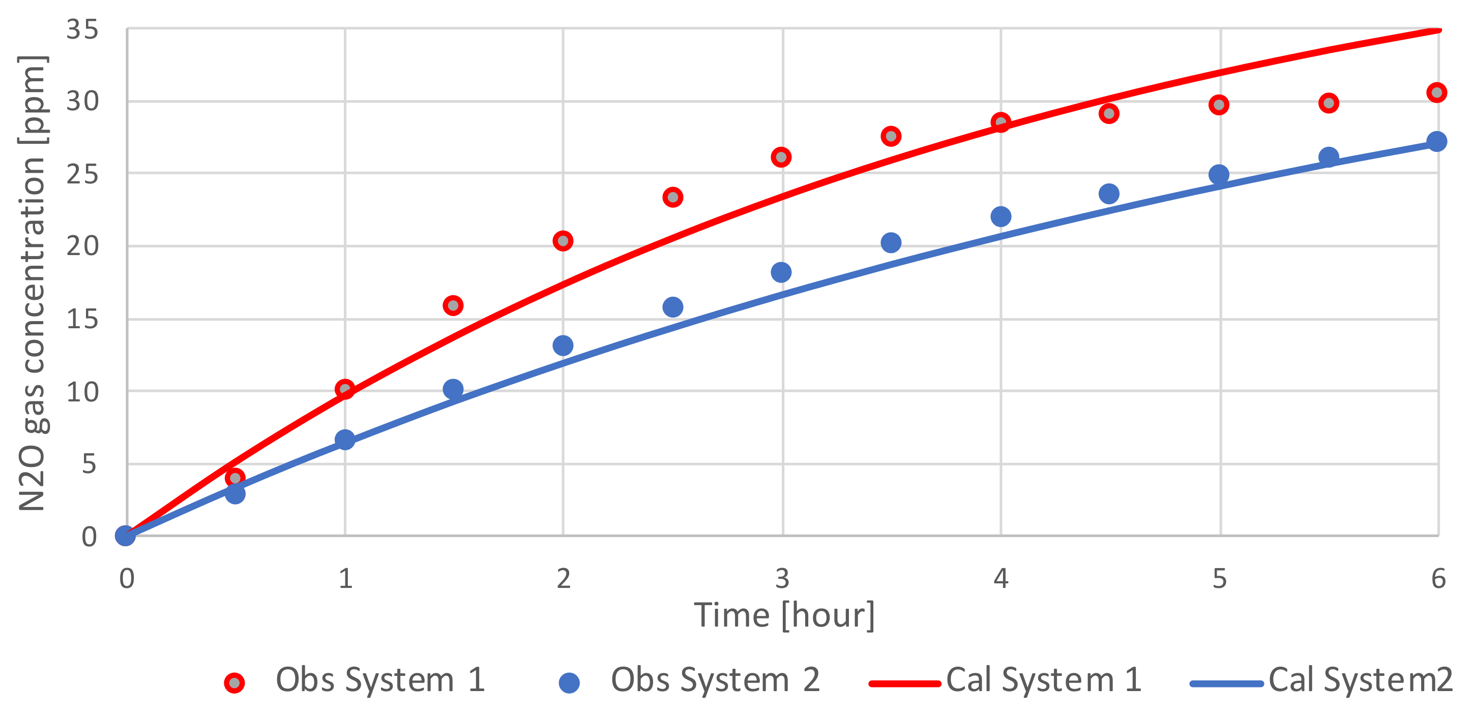
3.1. Diffusion Coefficient of the Silicone Membrane

The results of the gas diffusion test and simulation process are shown in Figure 5. Depending on the variations in the concentration gradient between the gas chamber and silicone tubes, the graphs of the observed N₂O gas accumulation rate in the silicone tubes changed from being steep to moderate. Because of the different internal volumes of the two gas-monitoring devices (system 1: 500 mL and system 2: 320.3 mL), the steepness of the two curves demonstrates steeper N₂O gas accumulation in system 1 than in system 2. In the simulation output, the temporal variation in calculated gas concentrations in both systems match with the measured values. For the N₂O gas, the diffusion coefficient of the silicone membrane (D_slcn) was 1.1 × 10⁻⁸ cm²/s according to the steps resolved in the difference equations (Equation (3)).

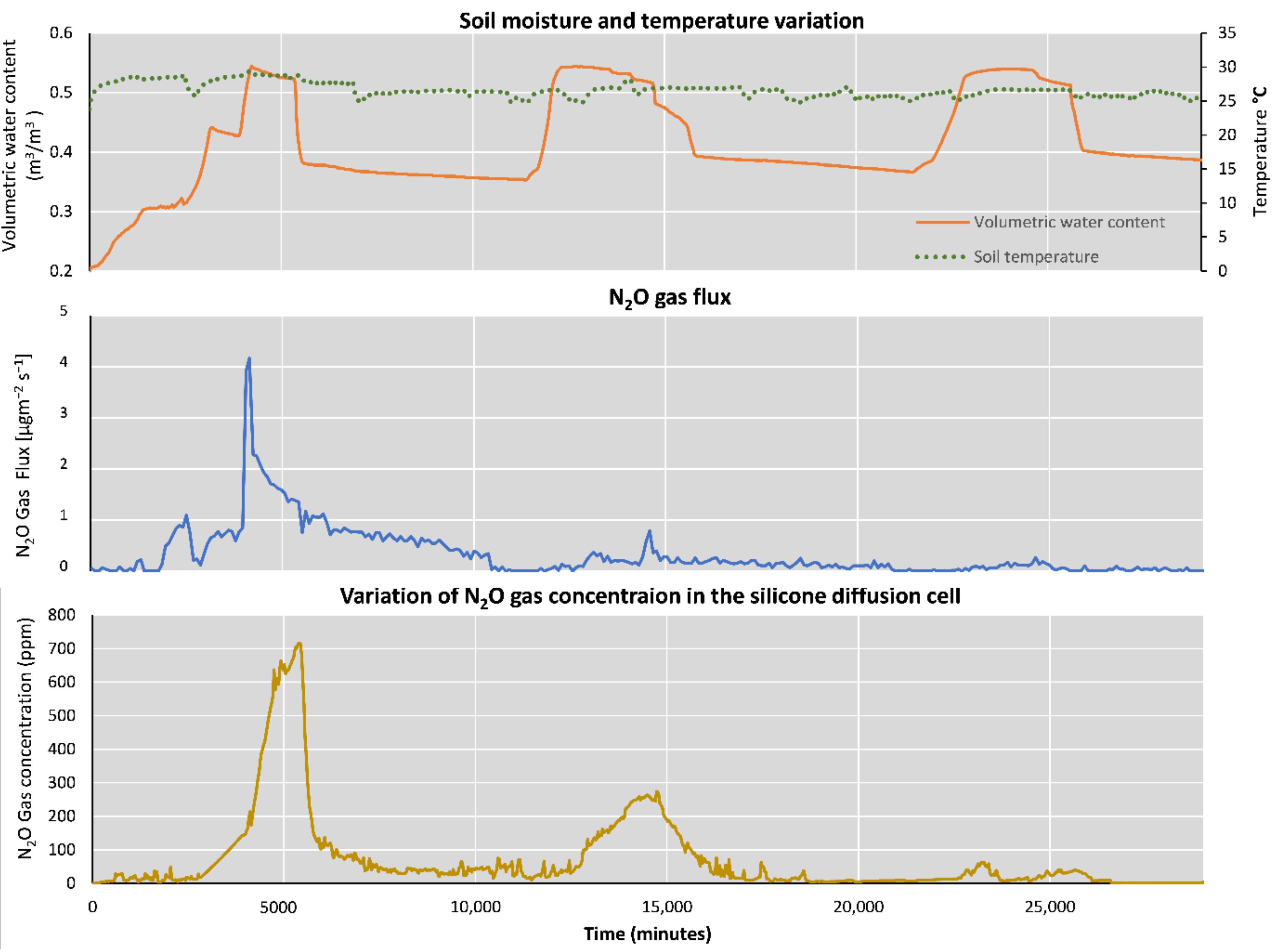
3.2. Results of the Variations in N₂O Gas Concentration in the Silicone diffusion cell and N₂O Gas flux of the Headspace of Experiment 1 and 2

Considering experiments 1 and 2, the variations in the gas flux from soil surface and the gas concentrations in the silicone diffusion cell show similar patterns during the irrigation and drainage events (Figure 6 and Figure 7).

During the saturation events, higher gas production was observed in both experiments than during the drainage period. As discussed in previous studies [50,51,52,53], during saturation events, microbes produce more N₂O gas via nitrification and denitrification processes, since the soil moisture regulates the oxygen availability in the soil pores. Zheng et al. [54] also demonstrated a similar N₂O gas variation pattern in in situ measurements testing the impacts of soil moisture on gas emissions on crop land. However, in this study, during the drainage period, considerably elevated gas levels were observed for a short period of time when the water filling the space in the soil pores was replaced when the soil gas changed its diffusion direction temporarily to be downwards. This condition, which was determined to be a function of soil gas diffusion under low water-filled pore spaces, disappeared soon after the drainage completion and was clearly shown in both experiments. In experiment 1, the drainage and saturation periods were both two days long, and water was allowed to drain with the help of gravity (faster draining process than experiment 2). A very sharp elevated gas level was observed at the beginning of the drainage period compared to that in experiment 2, where the drainage process was carried out at a lower rate. The graphs showing the volumetric water content in Figure 6 and Figure 7 also demonstrate the two drainage flow rates in experiments 1 and 2.

In both experiments, at peak levels, the variations in the N₂O gas concentration levels that were measured in the silicone diffusion cell were approximately 10 times higher than they were in the measurements for the headspace concentration. This characteristic explains the possibility of using low-cost and less precise gas-monitoring devices to monitor soil gas levels compared with the costly surface chamber methods [25] associated with high-precision gas measurement events for determining trace gas levels. During the two experiments, the average soil temperatures were 22.6 ± 0.41 °C and 26.52 ± 1.01 °C for experiments 1 and 2, respectively.

3.3. Results of the Simulation Steps of the Soil N₂O Gas Level Prediction

For both experiments 1 and 2, the series of C_soil were shifted to an earlier position (time lag) in the time series compared to the C_si series (Figure 8 and Figure 9). Because of the diffusion coefficient of the silicone diffusion cell, theoretically, the simulated values of soil N₂O should appear earlier on in the time series than the time points of the corresponding gas levels of C_si, and this time lag confirms the condition. The time lag was the result of the repeated simulation steps that were conducted to achieve the overlapping C_ssi and C_si series. Since C_ssi is simulated from C_soil, the accuracy of the simulation process is confirmed by the clearly overlapping C_si series on the C_ssi series in both experiments. In the case of experiment 1, the high C_ssi peaks that occurred soon after drainage began were smaller than those that were observed for C_si. We considered that these peaks could be caused by gas diffusion, as well as by rapid changes in the soil gas pressure under the forcible drainage. Therefore, these peaks could not be calculated by solving the diffusion equation.

According to the graphical descriptions of Figure 10 and Figure 11 for experiments 1 and 2, the highest agreement level between CFcu and MFcu is shown by soil gas diffusivity models 4 and 5. The results (

Table 1. Results of the accuracy tests conducted for CFcu with all models with MFcu.

Experiment	Accuracy Test	Model
		1		2	3	4		5		6
1	SMAPE (%)	16.45		31.85	20.02	8.18		10.18		19.72
	d	0.9954		0.9905	0.9965	0.9996		0.9994		0.9964
2	SMAPE (%)	12.63		27.89	18.18	10.73		8.02		20.65
	d	0.9947		0.9844	0.9924	0.9992		0.9997		0.9893
Color scale of SMAPE: Symmetric mean absolute percentage error (%).
		0	5	10	15	20	25	30	35
Color scale of d: Willmott’s agreement index (goodness of fit (scale 0–1) of the model’s output (CF) to the measured cumulative N2O flux (MF)).
		0.9	0.92	0.94	0.96	0.98		1

) of the accuracy tests (SMAPE: symmetric mean absolute percentage error (%), d: Willmott’s agreement index) for model fitting with MFcu also confirm the output of said graphical explanation. Among the tested characteristic-based soil gas diffusivity models for soil water, models 4 and 5 demonstrate lower SMAPE (%) values (experiment 1: 8.18%, 10.18%; experiment 2: 10.73%, 8.02%) and higher d values (experiment 1: 0.9996, 0.9994; experiment 2: 0.9992, 0.9997). The independent models for the different soil types (models 1, 2, and 3) showed higher SMAPE and lower d values for both experiments. Therefore, according to the selected soil category, by considering the common simulation approach for predicting soil surface N₂O flux from the soil gas levels, soil gas diffusivity models 4 and 5 are the most appropriate regardless of whether or not the water supply method is controlled.

Considering the results of the two experiments, a simulation approach for predicting N₂O soil surface flux according to measured soil N₂O gas data was successfully carried out at the laboratory level. However, additional experiments need to be conducted on cultivated land before this method is adopted at the field level.

The tested method, including the arrangement of its hardware arrangement together with the simulation steps, makes it easier to estimate soil N₂O emissions once the gas diffusion coefficients of the silicone membrane and the soil have been determined. Compared to closed-chamber methods, the tested method requires less accessories for gas sampling and circulating and uses low-cost measurement devices. As a passive gas sampling unit, the special characteristics (water repellency, structural stability of the wall, and higher gas permeability) of the silicone diffusion cell allow it to be layered under the soil. This keeps the upper surface free of gas-sampling devices and enables natural soil gas diffusion to the air. Moreover, the gas sampler does not require operating power or intensive maintenance, which allows it to be used for long-term monitoring.

The gas sampling technique of the proposed simulation method has demonstrated the function of fewer gas sampling structures above the ground, which allows the natural gas diffusion process from the soil surface. Reflecting the current greenhouse gas sampling and analyzing techniques, compared to the precise eddy covariance technique [55,56], the chamber enclosure method was greatly applied because of the relative inexpensiveness and simplicity of the measurement mechanism [57,58]. However, the artifacts of established gas sampling structures (chamber artifacts) form errors and higher uncertainty in the ultimate results [59] via the altered diffusion gradient [60] and pressure artifacts [61,62]. The long covering period of the transparent chamber results in higher internal temperatures, and the opaque chamber method was proposed for blocking the impact of the light and tested for CO₂ [63] and CH₄ [64] gases. For the N₂O flux, the DN-based opaque static chamber measurement method has been tested to further improvement of accuracy in the opaque chamber [65]. Therefore, the tested method including soil-entombed silicone diffusion cell can minimize the artifacts and biases made by above-ground gas sampling structures of the chamber methods.

In the simulation steps, there are only two stages of analysis in the implicit finite difference method, which are based on the volumetric water content of the soil and the diffusion coefficients of the silicone membrane and the soil. Moreover, special models and solution methods are not required, and only a simple solution for diffusion equation analysis is enough for estimating the flux. Therefore, said parameters for the soil and gas sampler are found, and the analysis of the replicated data from various sampling points can be continued effortlessly. As a low-cost method, it is more likely that this method will be adopted at the field level, and this method increases the number of measurement points per field, accelerating the estimation of N₂O gas emission activities in agricultural fields.

4. Conclusions

We tested a simulation method for estimating the soil surface flux of N₂O gas from measured soil atmospheric gas levels. The methodology consisted of three steps: determining the diffusion coefficient of the silicone membrane, monitoring N₂O gas variations in the soil and gas flux from soil surface, and carrying out the simulation steps for predicting the surface emissions from the measured soil gas levels. The diffusion coefficient of the silicone membrane for the N₂O gas was determined to be 1.1 × 10⁻⁸ cm²/s by solving a diffusion equation. In the first stage of simulation, D_slcn was used to predict the variation in the soil N₂O gas level according to the measured N₂O gas concentrations in a silicone diffusion cell by solving the gas diffusion equation via the implicit finite difference analysis method. In the second stage, using soil gas diffusion coefficients from six soil gas diffusivity models, the N₂O gas flux from the soil surface emissions was predicted from the predicted soil gas levels. At the laboratory level, we successfully simulated the cumulative values of the predicted soil surface N₂O flux and confirmed the good agreement with the measured cumulative flux graphically and statistically in both experiments. From the tested six soil gas diffusivity models, models 4 and 5 demonstrated lower SMAPE (%) and higher d values for CFcu and Mfcu in both experiments. The results of the two experiments using varying soil saturation methods and durations in the fertilized soil samples confirmed that the simulation methodology was acceptable for predicting the surface flux from measured soil gas levels. The overlapping CFcu and Mfcu curves and the results of the statistical tests (SMAPE (%) and d) demonstrate how expensive conventional N₂O flux estimation methods can be replaced with the use of low-cost gas-monitoring devices for soil gas measurements with gas flux simulation steps. Further field-level studies are needed before the simulation method is adopted for use in cultivated cropland.

References

1. Skiba, U.; Rees, B. Nitrous oxide, climate change and agriculture. CAB Rev. Perspect. Agric. Vet. Sci. Nutr. Nat. Resour. 2014, 9, 1–7. [Google Scholar] [CrossRef]
2. Mosier, A.R.; Syers, J.K.; Freney, J.R. Nitrogen fertilizer: An essential component of increased food, feed, and fiber production. In Agriculture and the Nitrogen Cycle: Assessing the Impacts of Fertilizer Use on Food Production and the Environment; Mosier, A.R., Syers, J.K., Freney, J.R., Eds.; SCOPE 65 Island Press: Washington, DC, USA, 2004; pp. 3–15. [Google Scholar]
3. Kaur, R.; Kaur, S. Biological alternates to synthetic fertilizers: Efficiency and future scopes. Indian J. Agric. Res. 2018, 52, 587–595. [Google Scholar] [CrossRef]
4. Gollner, G.; Starz, W.; Friedel, J.K. Crop performance, biological N fixation and pre-crop effect of pea ideotypes in an organic farming system. Nutr. Cycl. Agroecosyst. 2019, 115, 391–405. [Google Scholar] [CrossRef] [Green Version]
5. USGCRP (U.S. Global Change Research Program). Climate Science Special Report: Fourth National Climate Assessment; Wuebbles, D.J., Fahey, D.W., Hibbard, K.A., Dokken, D.J., Stewart, T.K., Maycock, B.C., Eds.; U.S. Global Change Research Program: Washington, DC, USA, 2017; Volume I. [Google Scholar] [CrossRef] [Green Version]
6. Global Annual Surface Man Abundances (2020) and Trends of Key Greenhouse Gases from the GAW In-Situ Observational Network for GHG. The Averaging Method is Described in GAW Report No. 184 9. Available online: https://gaw.kishou.go.jp/static/publications/bulletin/Bulletin2019/ghg-bulletin-16.pdf (accessed on 20 April 2022).
7. Ravishankara, A.R.; Daniel, J.; Portmann, R. Nitrous Oxide (N2O): The Dominant Ozone-Depleting Substance Emitted in the 21st Century. Science 2009, 326, 123–125. [Google Scholar] [CrossRef] [Green Version]
8. Zschornack, T.; Rosa, C.; Reis, C.; Pedroso, G.; Camargo, E.; Santos, D.; Boeni, M.; Bayer, C. Soil CH4 and N2O Emissions from Rice Paddy Fields in Southern Brazil as Affected by Crop Management Levels: A Three-Year Field Study. Rev. Bras. Ciênc. Solo 2018. [Google Scholar] [CrossRef] [Green Version]
9. Wang, B.; Brewer, P.E.; Shugart, H.H.; Lerdau, M.T.; Allison, S.D. Soil aggregates as biogeochemical reactors and implications for soil-atmosphere exchange of greenhouse gases—A concept. Glob. Chang. Biol. 2019, 25, 373–385. [Google Scholar] [CrossRef] [PubMed]
10. Chesworth, W. Encyclopedia of Soil Science; Springer: Dorderecht, The Netherlands, 2009; p. 902. [Google Scholar]
11. Smith, K.A.; Ball, T.; Conen, F.; Dobbie, K.E.; Rey, A. Exchange of greenhouse gases between soil and atmosphere: Interactions of soil physical factors and biological processes. Eur. J. Soil Sci. 2018, 69, 2–4. [Google Scholar] [CrossRef]
12. Barnard, R.; Leadley, P.W.; Hungate, B.A. Global change, nitrification, and denitrification: A review. Glob. Biogeochem. Cycles. 2005, 19, GB1007. [Google Scholar] [CrossRef]
13. Van Groenigen, K.J.; Osenberg, C.W.; Hungate, B.A. Increased soil emissions of potent greenhouse gases under increased atmospheric CO2. Nature 2011, 475, 214–216. [Google Scholar] [CrossRef]
14. Wolf, B.; Chen, W.; Brüggemann, N.; Zheng, X.; Pumpanen, J.; Butterbach-Bahl, K. Applicability of the soil gradient method for estimating soil-atmosphere CO2, CH4, and N2O fluxes for steppe soils in Inner Mongolia. J. Plant Nutr. Soil Sci. 2011, 174, 359–372. [Google Scholar] [CrossRef]
15. Dijkstra, F.A.; Prior, S.A.; Runion, G.B.; Torbert, H.A.; Tian, H.Q.; Lu, C.Q.; Venterea, R.T. Effects of elevated carbon dioxide and increased temperature on methane and nitrous oxide fluxes: Evidence from field experiments. Front. Ecol. Environ. 2012, 10, 520–527. [Google Scholar] [CrossRef]
16. Ma, F.; Li, M.; Wei, N.; Dong, L.; Zhang, X.; Han, X.; Li, K.; Guo, L. Impacts of Elevated Atmospheric CO2 and N Fertilization on N2O Emissions and Dynamics of Associated Soil Labile C Components and Mineral N in a Maize Field in the North China Plain. Agronomy 2022, 12, 432. [Google Scholar] [CrossRef]
17. Sustainable Development Goals. Available online: https://www.un.org/sustainabledevelopment/climate-change/ (accessed on 15 April 2022).
18. Denmead, O.T. Approaches to measuring fluxes of methane and nitrous oxide between landscapes and the atmosphere. Plant Soil. 2008, 309, 5–24. [Google Scholar] [CrossRef]
19. Butterbach-Bahl, K.; Sander, B.O.; Pelster, D.; Díaz-Pinés, E. Quantifying Greenhouse Gas Emissions from Managed and Natural Soils. In Methods for Measuring Greenhouse Gas Balances and Evaluating Mitigation Options in Smallholder Agriculture; Rosenstock, T., Rufino, M., Butterbach-Bahl, K., Wollenberg, L., Richards, M., Eds.; Springer: Cham, Switzerland, 2016. [Google Scholar] [CrossRef] [Green Version]
20. Maljanen, M.; Liikanen, A.; Silvola, J.; Martikainen, P.J. Measuring N2O emissions from organic soils by closed chamber or soil/snow N2O gradient methods. Eur. J. Soil Sci. 2003, 54, 625–631. [Google Scholar] [CrossRef]
21. Martikainen, P.J.; Nykänen, H.; Crill, P.; Silvola, J. Effect of a lowered water table on nitrous oxide fluxes from northern peatlands. Nature 1993, 366, 51–53. [Google Scholar] [CrossRef]
22. Nykänen, H.; Alm, J.; Lång, K.; Silvola, J.; Martikainen, P.J. Emissions of CH4, N2O and CO2 from a virgin fen and a fen drained for grassland in Finland. J. Biogeogr. 1995, 22, 351–357. [Google Scholar] [CrossRef]
23. Flessa, H.; Wild, U.; Klemisch, M.; Pfadenhauer, J. Nitrous oxide and methane fluxes from organic soils under agriculture. Eur. J. Soil Sci. 1998, 49, 327–335. [Google Scholar]
24. Chikowo, R.; Zingore, S.; Snapp, S.; Johnston, A. Farm typologies, soil fertility variability and nutrient management in smallholder farming in Sub-Saharan Africa. Nutr. Cycl. Agroecosyst. 2014, 100, 1–18. [Google Scholar] [CrossRef]
25. Breuer, L.; Papen, H.; Butterbach-Bahl, K. N2O-emission from tropical forest soils of Australia. J. Geophys. Res. 2000, 105, 26353–26378. [Google Scholar] [CrossRef]
26. Butterbach-Bahl, K.; Papen, H.; Rennenberg, H. Impact of gas transport through rice cultivars on methane emission from rice paddy fields. Plant Cell Environ. 1997, 20, 1175–1183. [Google Scholar] [CrossRef]
27. Butterbach-Bahl, K.; Gasche, R.; Breuer, L.; Papen, H. Fluxes of NO and N2O from temperate forest soils: Impact of forest type, N deposition and of liming on the NO and N2O emissions. Nutr. Cycl. Agroecosyst. 1997, 48, 79–90. [Google Scholar] [CrossRef]
28. Bandara, K.M.T.S.; Sakai, K.; Nakandakari, T.; Yuge, K. A Low-Cost NDIR-Based N2O Gas Detection Device for Agricultural Soils: Assembly, Calibration Model Validation, and Laboratory Testing. Sensors 2021, 21, 1189. [Google Scholar] [CrossRef]
29. Pihlatie, M.; Pumpanen, J.; Rinne, J.; Ilvesniemi, H.; Simojoki, A.; Hari, P.; Vesala, T. Gas concentration driven fluxes of nitrous oxide and carbon dioxide in boreal forest soil. Tellus B Chem. Phys. Meteorol. 2007, 59, 458–469. [Google Scholar] [CrossRef]
30. Goffin, S.; Longdoz, B.; Maier, M.; Schack-Kirchner, H.; Aubinet, M. Soil Respiration in forest Ecosystems: Combination of a multilayer Approach and an Isotopic Signal Analysis. Commun. Agric. Appl. Biol. Sci. 2012, 72, 139–144. [Google Scholar]
31. Maier, M.; Longdoz, B.; Laemmel, T.; Schack-Kirchner, H.; Lang, F. 2D profiles of CO2, CH4, N2O and gas diffusivity in a well aerated soil: Measurement and Finite Element Modeling. Agric. Met. 2017, 247, 21–33. [Google Scholar] [CrossRef]
32. Jacinthe, P.-A.; Dick, W.A. Use of silicone tubing to sample nitrous oxide in the soil atmosphere. Soil Biol. Biochem. 1996, 28, 721–726. [Google Scholar] [CrossRef]
33. Jacinthe, P.-A.; Groffman, P.M. Silicone rubber sampler to measure dissolved gases in saturated soils and waters. Soil Biol. Biochem. 2001, 33, 907–912. [Google Scholar] [CrossRef]
34. Kammann, C.; Grünhage, L.; Jäger, H.J. A new sampling technique to monitor concentrations of CH4, N2O and CO2 in air at well-defined depths in soils with varied water potential. Eur. J. Soil Sci. 2001, 52, 297–303. [Google Scholar] [CrossRef]
35. Maier, M.; Machacova, K.; Lang, F.; Svobodova, K.; Urban, O. Combining soil and tree-stem flux measurements and soil gas profiles to understand CH4 pathways in Fagus sylvatica forests. J. Plant Nutr. Soil Sci. 2018, 181, 31–35. [Google Scholar] [CrossRef] [Green Version]
36. Maier, M.; Gartiser, V.; Schengel, A.; Lang, V. Long Term Soil Gas Monitoring as Tool to Understand Soil Processes. Appl. Sci. 2020, 10, 8653. [Google Scholar] [CrossRef]
37. Marinov, M.; Nikolov, G.; Gieva, E.; Ganev, B. Improvement of NDIR carbon dioxide sensor accuracy. In Proceedings of the 38th International Spring Seminar on Electronics Technology (ISSE), Eger, Hungary, 6–10 May 2015; pp. 466–471. [Google Scholar]
38. Yasuda, T.; Yonemura, S.; Tani, A. Comparison of the characteristics of small commercial NDIR CO2 sensor models and development of a portable CO2 measurement device. Sensors 2012, 12, 3641–3655. [Google Scholar] [CrossRef] [PubMed] [Green Version]
39. Honeycutt, W.T.; Ley, M.T.; Materer, N.F. Precision and Limits of Detection for Selected Commercially Available, Low-Cost Carbon Dioxide and Methane Gas Sensors. Sensors 2019, 19, 3157. [Google Scholar] [CrossRef] [Green Version]
40. Hodgkinson, J.; Smith, R.; Wo, H.; Saffell, J.R.; Tatam, R.P. A low cost, optically efficient carbon dioxide sensor based on nondispersive infra-red (NDIR) measurement at 4.2 μm. In Optical Sensing and Detection II; International Society for Optics and Photonics: Bellingham, WA, USA, 2012; Volume 8439, p. 843919. [Google Scholar]
41. Maier, M.; Schack-Kirchner, H. Using the gradient method to determine soil gas flux: A review. Agric. For. Meteorol. 2014, 192–193, 78–95. [Google Scholar] [CrossRef]
42. Atsuhiro, T.; Tetsuya, H.; Hiroshi, A.T.; Yoshihiro, F. Analytical estimation of the vertical distribution of CO2 production within soil: Application to a Japanese temperate forest. Agric. For. Meteorol. 2004, 126, 223–235. [Google Scholar] [CrossRef]
43. Schack-Kirchner, H.; Kublin, E.; Hildebrand, E.E. Finite-Element Regression to Estimate Production Profiles of Greenhouse Gases in Soils. Vadose Zone J. 2011, 10, 169–183. [Google Scholar] [CrossRef]
44. Buckingham, E. Contributions to Our Knowledge of the Aeration of Soils; USDA Burr Soil Bulletin, 25; US Government Printing Office: Washington, DC, USA, 1904. [Google Scholar]
45. Millington, R.J.; Quirk, J.M. Transport in porous media. In Transactions of the 7th International Congress of Soil Science; Van Beren, F.A., Ed.; Elsevier: Amsterdam, The Netherlands, 1960; pp. 97–106. [Google Scholar]
46. Millington, R.J.; Quirk, J.M. Permeability of porous solids. Trans. Faraday Soc. 1961, 57, 1200–1207. [Google Scholar] [CrossRef]
47. Moldrup, P.T.; Olesen, J.; Gamst, P.; Schjønning, P.; Yamaguchi, T.; Rolston, D.E. Predicting the gas diffusion coefficient in repacked soil: Water-induced linear reduction model. Soil Sci. Soc. Am. J. 2000, 64, 1588–1594. [Google Scholar] [CrossRef]
48. Moldrup, P.T.; Olesen, P.; Schjønning, P.; Yamaguchi, T.; Rolston, D.E. Predicting the gas diffusion coefficient in undisturbed soil from soil water characteristics. Soil Sci. Soc. Am. J. 2000, 64, 94–100. [Google Scholar] [CrossRef]
49. Moldrup, P.; Kruse, C.W.; Rolston, D.E.; Yamaguchi, T. Modelling diffusion and reaction in soils: III. Predicting gas diffusivity from the Campbell soil water retention model. Soil Sci. 1996, 161, 366–375. [Google Scholar] [CrossRef]
50. Williams, E.J.; Hutchinson, G.L.; Fehsenfeld, F.C. NOx and N2O emissions from soil. Glob. Biogeochem. Cycles 1992, 4, 351–388. [Google Scholar] [CrossRef]
51. Poth, M.; Focht, D.D. 15N kinetic analysis of N2O production by Nitrosomonas europea: An examination of nitrifier denitrification. Appl. Environ. Microbiol. 1985, 49, 1134–1141. [Google Scholar] [CrossRef] [Green Version]
52. Davidson, E.A. Sources of nitric oxide and nitrous oxide following wetting of dry soil. Soil Sci. Soc. Am. J. 1992, 56, 95–102. [Google Scholar] [CrossRef]
53. Davidson, E.A. Soil water content and the ratio of nitrous oxide to nitric oxide emitted from soil. In The Biogeochemistry of Global Change: Radiatively Active Trace Gases; Oremland, R.S., Ed.; Chapman & Hall: New York, NY, USA, 1992. [Google Scholar]
54. Xunhua, Z.; Mingxing, W.; Yuesi, W.; Renxing, S.; Gou, J.; Jing, L.; Jisheng, J.; Laotu, L. Impacts of soil moisture on nitrous oxide emission from croplands: A case study on the rice-based agro-ecosystem in Southeast China. Chemosphere—Glob. Chang. Sci. 2000, 2, 207–224. [Google Scholar]
55. Wang, J.M.; Murphy, J.G.; Geddes, J.A.; Winsborough, C.L.; Basiliko, N.; Thomas, S.C. Methane fluxes measured by eddy covariance and static chamber techniques at a temperate forest in central Ontario, Canada. Biogeosciences 2013, 10, 4371–4382. [Google Scholar] [CrossRef] [Green Version]
56. Kroon, P.S.; Hensen, A.; Jonker, H.J.J.; Ouwersloot, H.G.; Vermeulen, A.T.; Bosveld, F.C. Uncertainties in eddy covariance flux measurements assessed from CH4 and N2O observations. Agric. For. Meteorol. 2010, 150, 806–816. [Google Scholar] [CrossRef] [Green Version]
57. Cao, G.; Xu, X.; Long, R.; Wang, Q.; Wang, C.; Du, Y.; Zhao, X. Methane emissions by alpine plant communities in the Qinghai-Tibet Plateau. Biol. Lett. 2008, 4, 681–684. [Google Scholar] [CrossRef] [Green Version]
58. Davidson, E.A.; Nepstad, D.C.; Ishida, F.Y.; Brando, P.M. Effects of an experimental drought and recovery on soil emissions of carbon dioxide, methane, nitrous oxide, and nitric oxide in a moist tropical forest. Glob. Chang. Biol. 2008, 14, 2582–2590. [Google Scholar] [CrossRef]
59. Davidson, E.A.; Savage, K.; Verchot, L.V.; Navarro, R. Minimizing artifacts and biases in chamber-based measurements of soil respiration. Agric. For. Meteorol. 2002, 113, 21–37. [Google Scholar] [CrossRef]
60. Conen, F.; Smith, K.A. An explanation of linear increases in gas concentration under closed chambers used to measure gas exchange between soil and the atmosphere. Eur. J. Soil Sci. 2000, 51, 111–117. [Google Scholar] [CrossRef]
61. Longdoz, B.; Yernaux, M.; Aubinet, M. Soil CO2 efflux measurements in a mixed forest: Impact of chamber disturbances, spatial variability and seasonal evolution. Glob. Chang. Biol. 2000, 6, 907–917. [Google Scholar] [CrossRef]
62. Lund, C.P.; Riley, W.J.; Pierce, L.L.; Field, C.B. The effects of chamber pressurization on soil-surface CO2 flux and the implications for NEE measurements under elevated CO2. Glob. Chang. Biol. 1999, 5, 269–281. [Google Scholar] [CrossRef]
63. Zou, J.; Huang, Y.; Zheng, X. Static opaque chamber-based technique for determination of net exchange of CO2 between terrestrial ecosystem and atmosphere. Chin. Sci. Bull. 2004, 49, 381. [Google Scholar] [CrossRef]
64. Junwei, L.; Jianghua, W. Gross photosynthesis explains the ‘artificial bias’ of methane fluxes by static chamber (opaque versus transparent) at the hummocks in a boreal peatland. Environ. Res. Lett. 2014, 9, 105005. [Google Scholar]
65. Lei, M.; Wei, Z.; Xunhua, Z.; Zhisheng, Y.; Han, Z.; Rui, W.; Bo, Z.; Kai, W.; Chunyan, L.; Guangmin, C.; et al. Attempt to correct grassland N2O fluxes biased by the DN-based opaque static chamber measurement. Atmos. Environ. 2021, 264, 118687. [Google Scholar] [CrossRef]
Figure 1. The main simulation steps for predicting the N2O flux from measured soil gas levels in the silicone diffusion cell.
Agriculture 12 01098 g001
Figure 2. Experimental setup for determining the diffusion coefficient of the silicone diffusion cell.
Agriculture 12 01098 g002
Figure 3. A diagram of the laboratory experimental setup for monitoring variations in the headspace and soil atmospheric N2O gas concentrations: (a) top-side water supply unit, (b) bottom-side water supply unit (Mariotte cell), (c) soil chamber, (d) soil region, (e) diffusion cell (silicone tube), (f) water drainage system, (g,j) membrane air-drying system, (h) low-cost NDIR gas-monitoring device, (i) FTIR device, (k) data logger connected to soil moisture and temperature sensors, (l) headspace of the soil chamber, and (m) ventilation system for chamber head space.
Agriculture 12 01098 g003
Figure 4. The repetitive simulation steps for obtaining the predicted N2O gas levels in soil.
Agriculture 12 01098 g004
Figure 5. Temporal variations in measured and calculated N2O gas concentrations in the silicone tubes of systems 1 and 2.
Agriculture 12 01098 g005
Figure 6. Temporal variations in the N2O gas concentrations in the silicone diffusion cell and N2O gas flux from the headspace, soil temperature, and moisture levels in experiment 1.
Agriculture 12 01098 g006
Figure 7. Temporal variations in the N2O gas concentrations in the silicone diffusion cell and N2O gas flux from the headspace, soil temperature, and moisture levels in experiment 2.
Agriculture 12 01098 g007
Figure 8. Temporal variations in measured and simulated N2O gas levels in the silicone diffusion cell with predicted soil gas levels for experiment 1.
Agriculture 12 01098 g008
Figure 9. Temporal variations in measured and simulated N2O gas levels in the silicone diffusion cell with predicted soil gas levels for experiment 2.
Agriculture 12 01098 g009
Figure 10. Experiment 1: temporal progression of the simulated cumulative N2O emissions in each of the soil gas diffusivity models with the observed emissions.
Agriculture 12 01098 g010
Figure 11. Experiment 2: temporal progression of the simulated cumulative N2O emissions for each of the soil gas diffusivity models with the observed emissions.
Agriculture 12 01098 g011