Article

Impact of Fiscal Expenditure on Farmers’ Livelihood Capital in the Ethnic Minority Mountainous Region of Sichuan, China

1
School of Economics, Southwestern University of Finance and Economics, Chengdu 611130, China
2
China Western Economic Research Institute, Southwestern University of Finance and Economics, Chengdu 611130, China
3
Sichuan Center for Rural Development Research, Sichuan Agricultural University, Chengdu 611130, China
*
Authors to whom correspondence should be addressed.
Agriculture 2022, 12(6), 881; https://doi.org/10.3390/agriculture12060881
Submission received: 15 April 2022 / Revised: 29 May 2022 / Accepted: 15 June 2022 / Published: 18 June 2022
(This article belongs to the Special Issue Ecological Restoration and Rural Economic Development)

Abstract

:
Poverty alleviation is the first battle to realize the rural revitalization strategy in China, and research on the sustainable livelihood of rural households is of great significance to solving the problem of rural poverty. Based on the sustainable livelihood framework, the reasonable scale and structure of fiscal expenditure is an inevitable requirement in producing sustainable livelihood capital toward this aim. In this study, the system Gaussian mixed model was used to analyze the impact of fiscal expenditure on farmers’ livelihoods. Representative survey data uses panel data from 48 counties across Liangshan Prefecture, Ganzi Prefecture, and Aba Prefecture in Sichuan, China. The results are as follows: (1) The average stock of human capital in 2010 to 2015 was the highest in the composition of farmers’ livelihood capital; (2) natural capital and physical capital were positively affected by the total scale of fiscal expenditure, agriculture, forestry, and water expenditure, and the former was negatively affected by general public service expenditure, education expenditure, social security and employment expenditure, and medical expenditure; (3) financial capital and the total amount of livelihood capital were positively affected by the total scale of fiscal expenditure, agriculture, forestry and water expenditure, education expenditure, social security and employment expenditure, and medical expenditure, and negatively affected by general public service expenditure; (4) human capital was positively affected by the total scale of fiscal expenditure, education expenditure, social security and employment expenditure, and medical expenditure; and (5) social capital was positively affected by agriculture, forestry and water expenditure, and education expenditure.

1. Introduction

China has a mountainous area of 6.66 million km2, including plateaus and hills, and this accounts for 69.4% of the total land area. The population in the mountainous regions accounts for more than one third of the country’s total population [1]. The majority of the mountainous areas are inhabited by poor and ethnic minorities—specifically, the 14 poverty-stricken areas in China are all mountainous. Since the 18th National Congress of the Communist Party of China, the number of the rural poor in the country has decreased from 98.99 million at the end of 2012 to 30.46 million at the end of 2017, which is a cumulative decrease of 68.53 million. Additionally, the incidence of poverty dropped from 10.2% at the end of 2012 to 3.1%, which is a cumulative decrease of 7.1% (data sources: http://www.gov.cn/xinwen/2018-02/01/content_5262903.htm (accessed on 14 April 2022)). Efforts to alleviate poverty have been extraordinary. However, those living in poverty are mainly concentrated in rural areas, especially in ethnic mountainous rural areas, which has made it difficult for China to build a prospering society all-round [2]. The key focus of accurate poverty alleviation, therefore, lies in the poverty alleviation of mountainous farmers. To this end, the level of farmers’ livelihood capital is a powerful indicator in evaluating poverty alleviation and poverty levels [3]. Consequently, improving the level of farmers’ livelihood capital and ensuring their way of life is sustainable has become a key point in solving the poverty issue [4].
The word “livelihood” in the dictionary means “a means of living”, and “capital” is the general name of all kinds of social and economic resources that human beings create material and spiritual wealth [5]. Livelihood capital contains natural capital, physical capital, social capital, human capital, and financial capital, among them. The natural capital refers to the storage of natural resources. The environment can attain favorable resource flows and services. Physical capital refers to the ecological economy in addition to the natural resources in the process of production capital. Human capital refers to the individual making a living and having the knowledge, skills, an ability to work, and health. Financial capital refers to the cash to spend on consumer goods and means of production and the personal loans available [6]. At the level of fiscal expenditure in the existing research, scholars pay more attention to the impact of fiscal expenditure on regional economic growth [7,8,9], the impact of fiscal expenditure on human capital, and the impact of public education investment on human capital and economy [10,11,12]. However, there is little uniformity across results. At the level of farmers’ livelihood, research on livelihood capital is based mainly on the calculation of livelihood capital [13,14,15], the impact of background vulnerability (external shock, seasonality, etc.) on the livelihood capital [16,17], livelihood strategy [18,19], and so on. The impact of fiscal expenditure on livelihood capital predominantly includes the following aspects: the impact of the scale of fiscal expenditure on farmers’ income. Many scholars have examined the overall impact of fiscal agriculture expenditure on farmers’ income from the national and regional levels, and most agree that fiscal agriculture expenditure has an impact on farmers’ income growth [20,21,22], while rural production expenditure in fiscal support for agriculture has a significant impact on the increase in farmers’ income [23]. The impact of the structure of financial support for agriculture on farmers’ income. Some studies show that the difference in the expenditure structure of financial support for agriculture will lead to different effects of the increase in farmers’ income [20]. Among them, the expenditure on supporting agriculture accounts for 66.7% of the total expenditure of financial agriculture, and the contribution rate to the variance of per-capita net income of farmers’ families is only 12.3%. Although the proportion of agricultural science and technology expenses is only 0.9%, the contribution rate to the variance of per-capita net income of farmers’ families is 20.6% [24]. However, some studies have found that fiscal agricultural production and relief expenditures are conducive to the increase in farmers’ incomes, while fiscal rural infrastructure expenditures have an inhibitory effect on farmers’ incomes [20]. Furthermore, rural financial support for agriculture and per-capita agricultural science and technology has negative effects on income [25]. The previous studies have deepened our understanding of the effects and mechanisms of fiscal expenditure on farmers’ income, which can help us better understand the relationship between fiscal expenditure policies and farmers’ livelihood capital. However, it should be noted that in addition to the fiscal support for farmers’ income, the financial infrastructure expenditure, cultural and educational expenditures, administrative expenditures, et cetera, may also affect farmers’ income and human capital through certain mechanisms.
Sichuan has a large population and 74.2% of it is mountainous. The regional development gap in this area is large. Among them, Ganzi Prefecture, Aba Prefecture, and Liangshan Prefecture (hereafter referred to as “the three states”) are representative of all poverty-stricken ethnic minority mountainous regions. The three states have higher altitudes, complex and diverse landforms, frequent natural disasters, and a very fragile ecological environment. Additionally, the three states are all ecological areas restricted in terms of development, facing the dual pressure of protecting the ecological environment and improving people’s livelihoods. Given this, the fiscal expenditure policy is an important measure in solving this tension. Based on the sustainable livelihood framework, this paper focuses on the impact of policies on livelihood capital. Research framework is shown in Figure 1.
Upon reading the relevant literature and combining the specifics of the study area, we designed the following research hypotheses (Figure 2):
H1: Natural capital is positively affected by the total fiscal expenditure scale (H1a), and the agriculture, forestry, and water expenditure (H1b) (Xin, 2012); and it is negatively affected by general public service expenditure (H1c), education expenditure (H1d), social security and employment expenditure (H1e), and medical expenditure (H1f) [12,26];
H2: Physical capital is positively affected by the total fiscal expenditure scale (H2a) and agriculture, forestry, and water expenditure (H2b) [27];
H3: Financial capital is positively affected by the total fiscal expenditure scale (H3a), general public service expenditure (H3b), agriculture and forestry water expenditure (H3c), education expenditure (H3d), social security and employment expenditure (H3e), and medical expenditure (H3f) [20,28,29];
H4: Human capital is positively affected by the total fiscal expenditure scale (H4a), education expenditure (H4b), social security and employment expenditure (H4c), and medical expenditure (H4d) [30,31];
H5: Social capital is positively affected by agriculture, forestry and water expenditure (H5a), and education expenditure (H5b) [32];
H6: The total livelihood capital is positively affected by the total fiscal expenditure scale (H6a), general public service expenditure (H6b), agriculture, forestry and water expenditure (H6c), education expenditure (H6d), social security and employment expenditure (H6e), and medical expenditure (H6f) [9,33].
H denotes human capital; N denotes natural capital; F denotes financial capital; P denotes physical capital; and S denotes social capital. Furthermore, scale denotes total financial expenditure; serv denotes the proportion of general public service expenditure; agri denotes the proportion of agriculture, forestry and water expenditure; edu denotes the proportion of education expenditure; soci denotes the proportion of social security and employment expenditure; and medi denotes the proportion of medical expenditure.

2. Materials and Methods

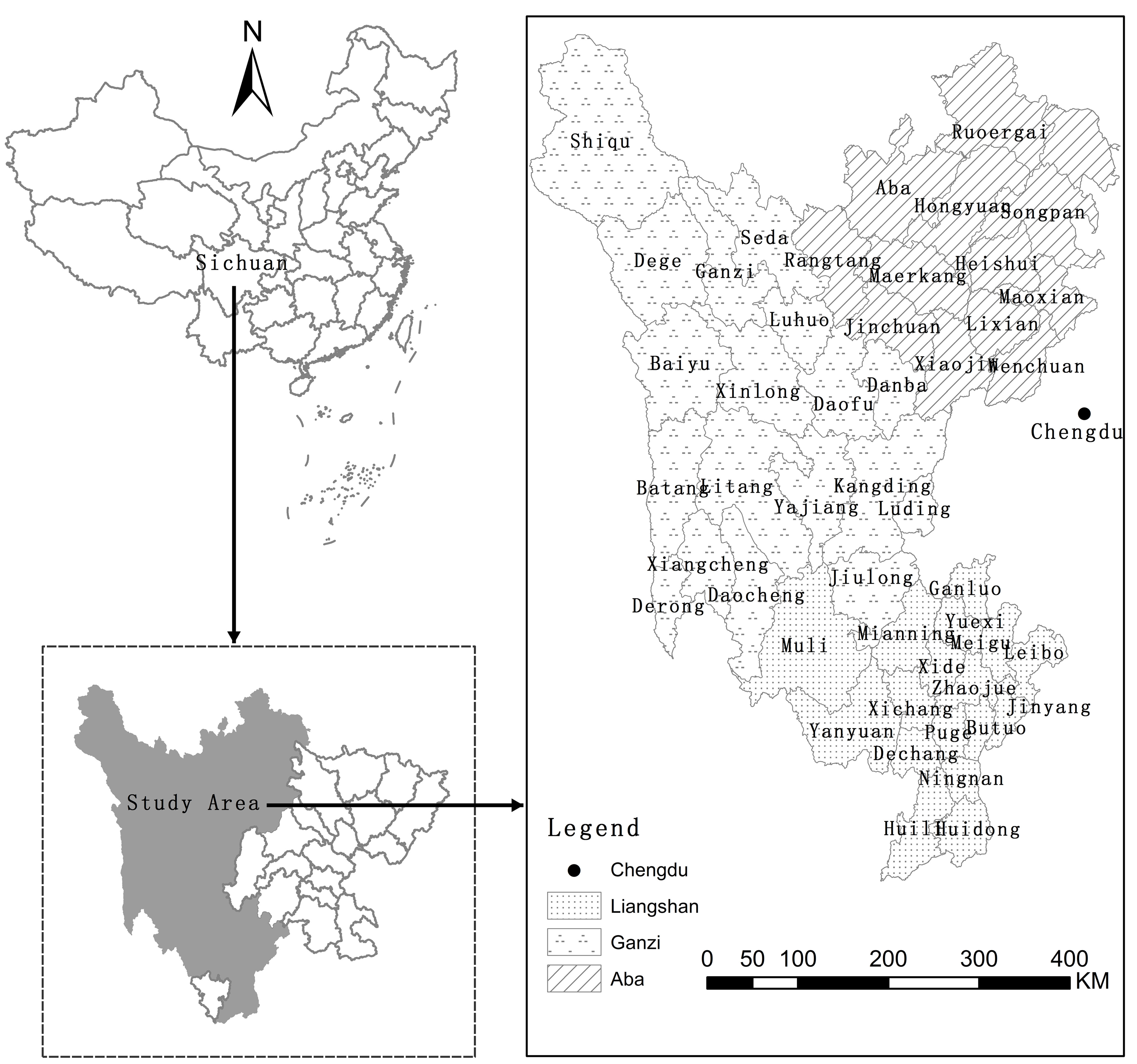
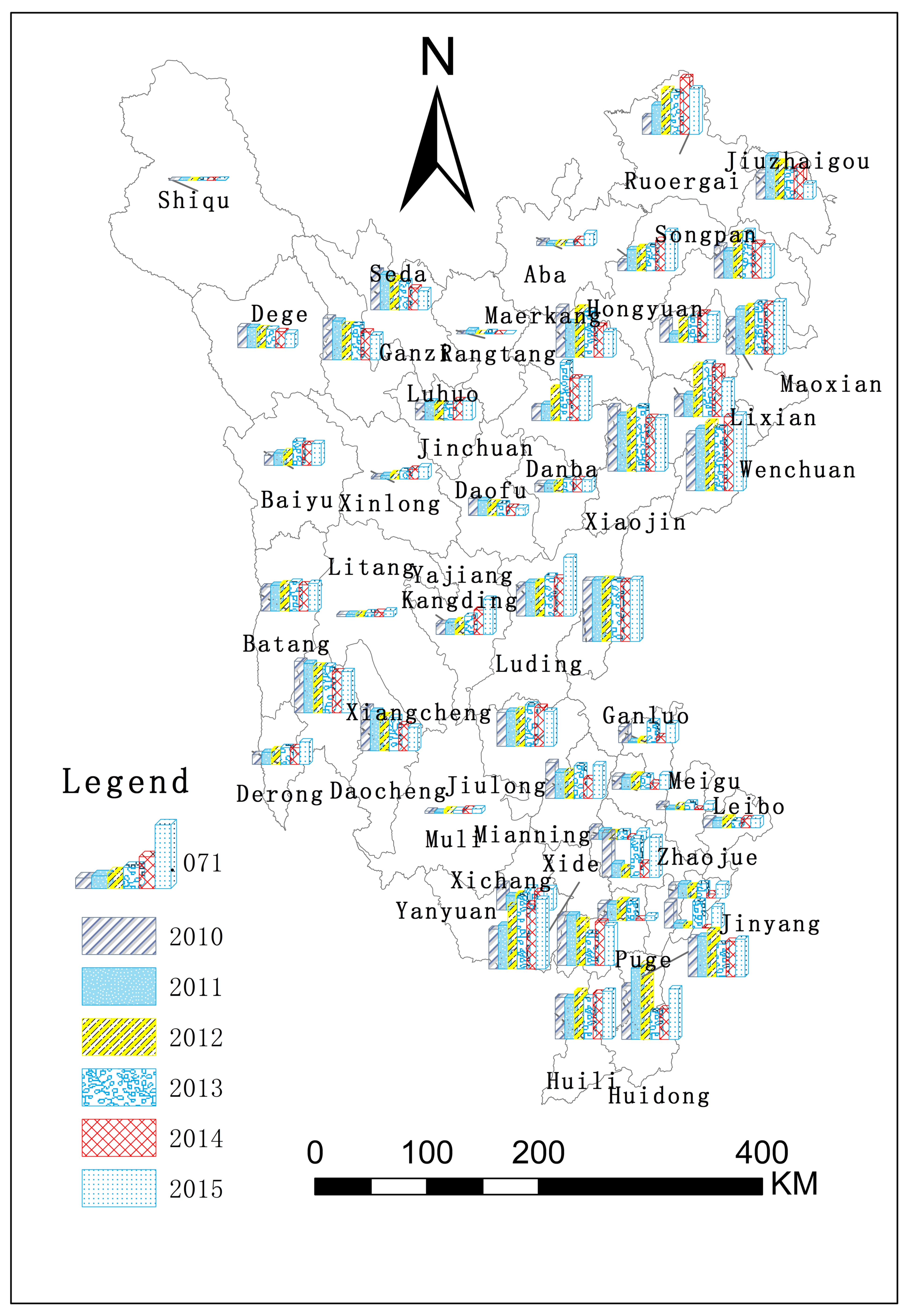
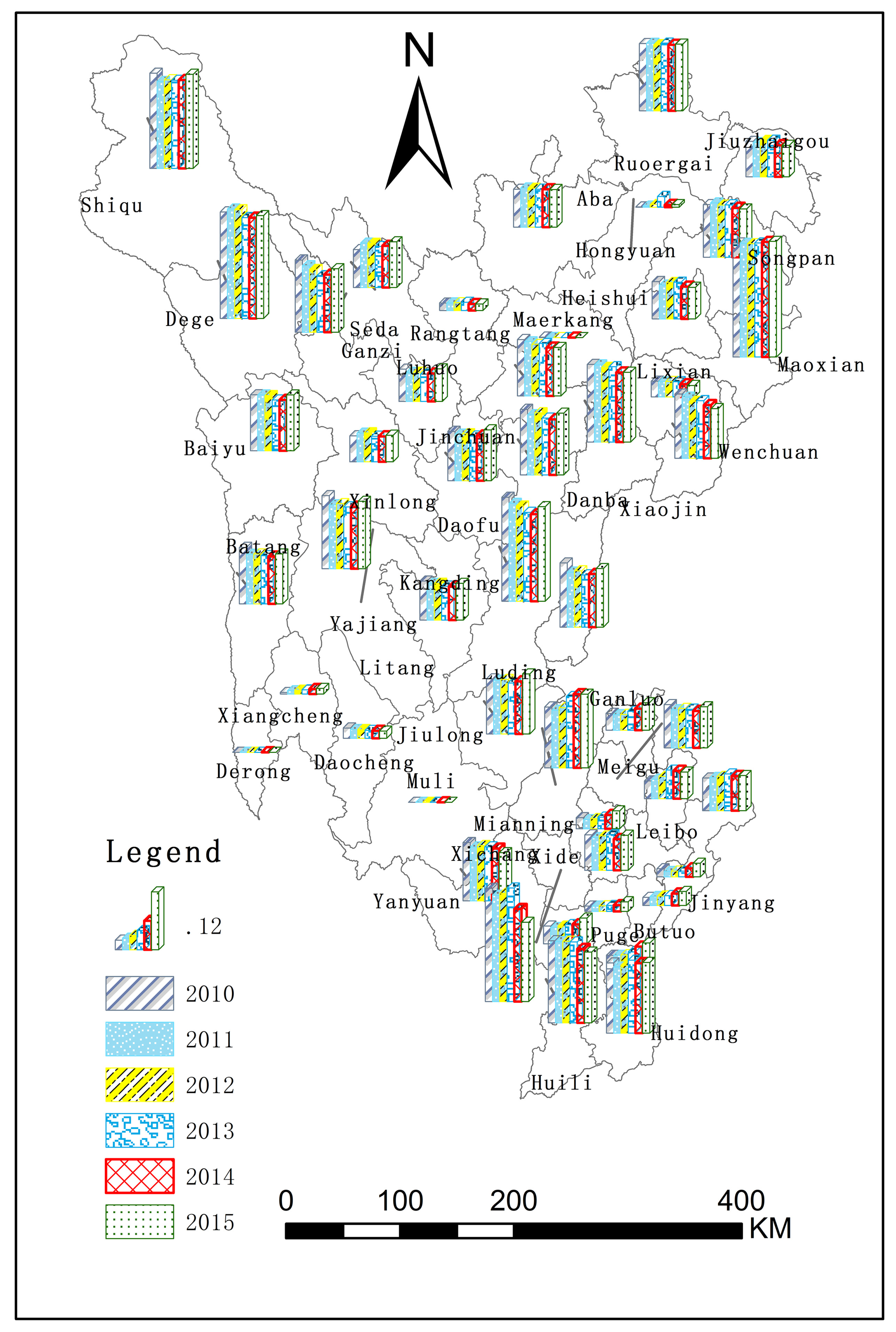
2.1. Overview of the Study Area

For research areas, this paper focuses on 47 counties across Liangshan Yi Autonomous Prefecture, Ganzi Tibetan Autonomous Prefecture, and Aba Tibetan and Qiang Autonomous Prefecture (Figure 3). Liangshan Prefecture is inhabited by the largest Yi population in China. There are 11 key counties in national poverty alleviation and development work. Aba Prefecture is the second largest Tibetan area and the main settlement of the Qiang people in Sichuan Province, with a minority population accounting for more than 75%. Furthermore, the 13 counties in the state are state-level subsidized counties in the hardship and remote areas. Ganzi Prefecture is the second largest Tibetan area in China, and 17 counties in the whole state are state-level subsidized counties in the hardship and remote areas. The population of the majority Tibetan areas accounts for 78.4%. The three states have wide-ranging and deep-seated poverty characteristics, and are typical, concentrated poverty-stricken minority areas.

2.2. Source of Data

The data on livelihood capital are derived from the survey data of farmers’ households from the Bureau of Statistics in Liangshan Prefecture, Ganzi Prefecture, and Aba Prefecture from 2010 to 2015. These data, such as fiscal expenditure, GDP, GDP per capita, investment in fixed assets of the whole society, minority population, highway mileage, and per-capita net income of farmers are derived from the Liangshan Prefecture Statistical Yearbook (2011–2016), the Ganzi Prefecture Statistical Yearbook (2011–2016), and the Aba Prefecture Statistical Yearbook (2011–2016).

2.3. Research Methods

2.3.1. Construction of Indicator System

(1)
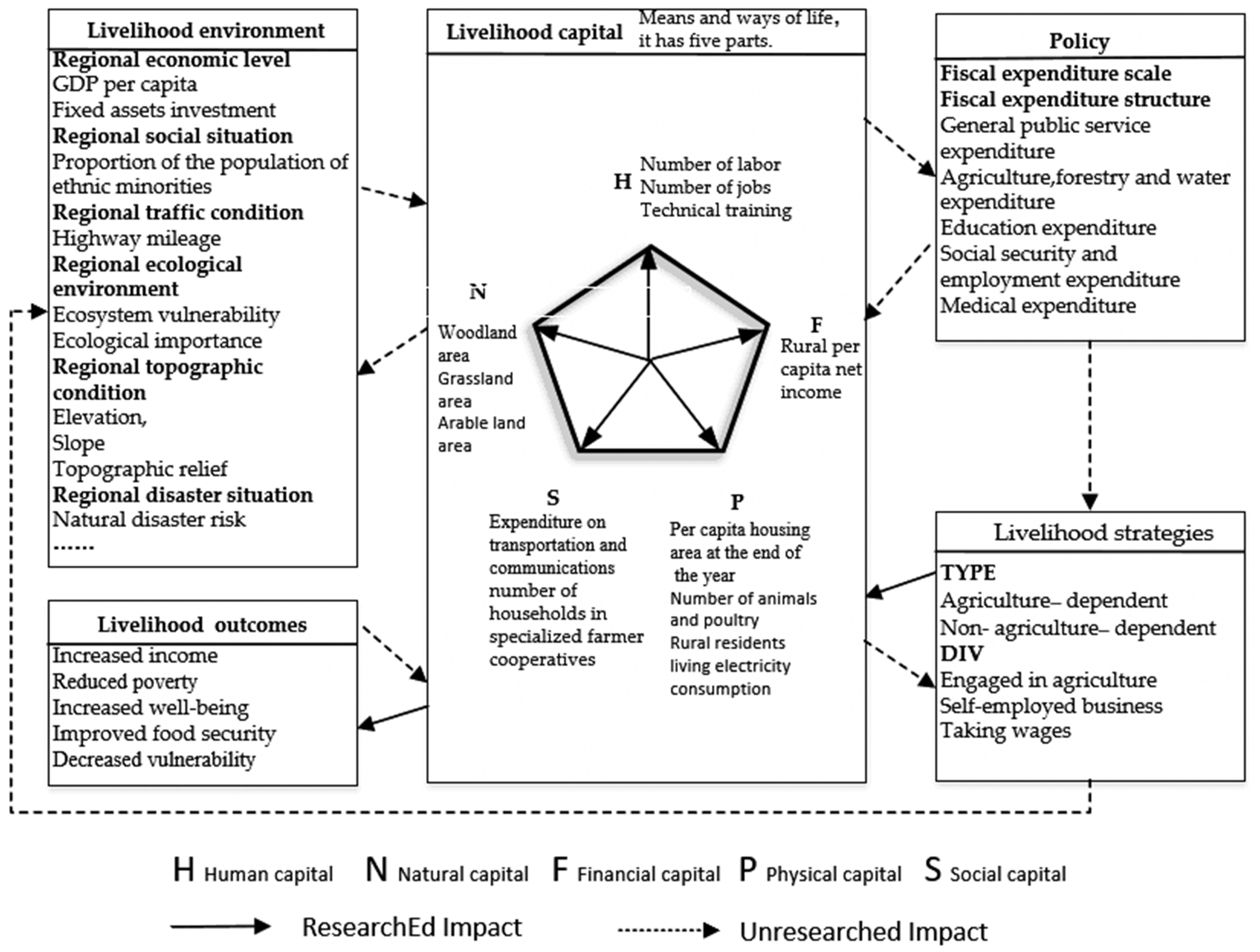
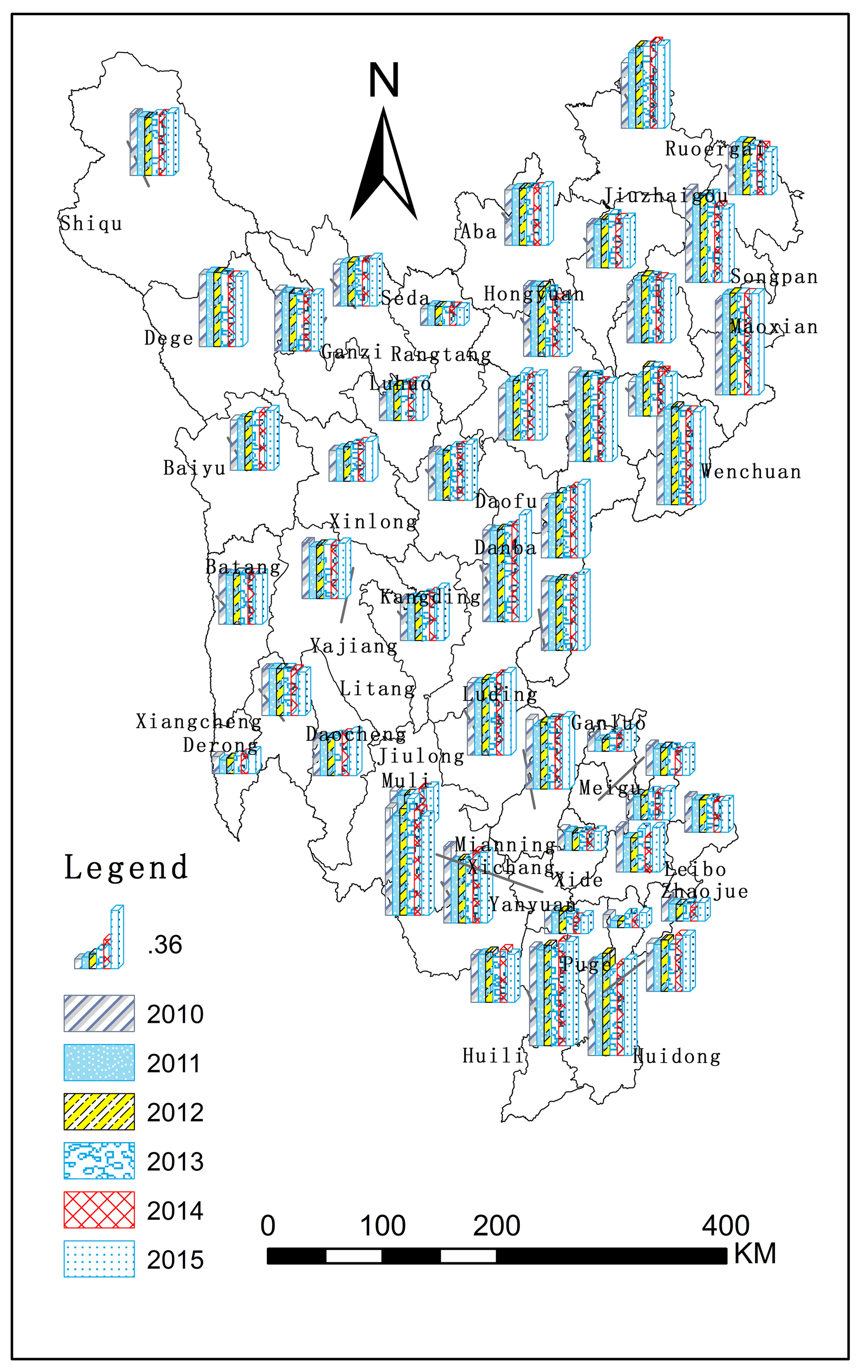
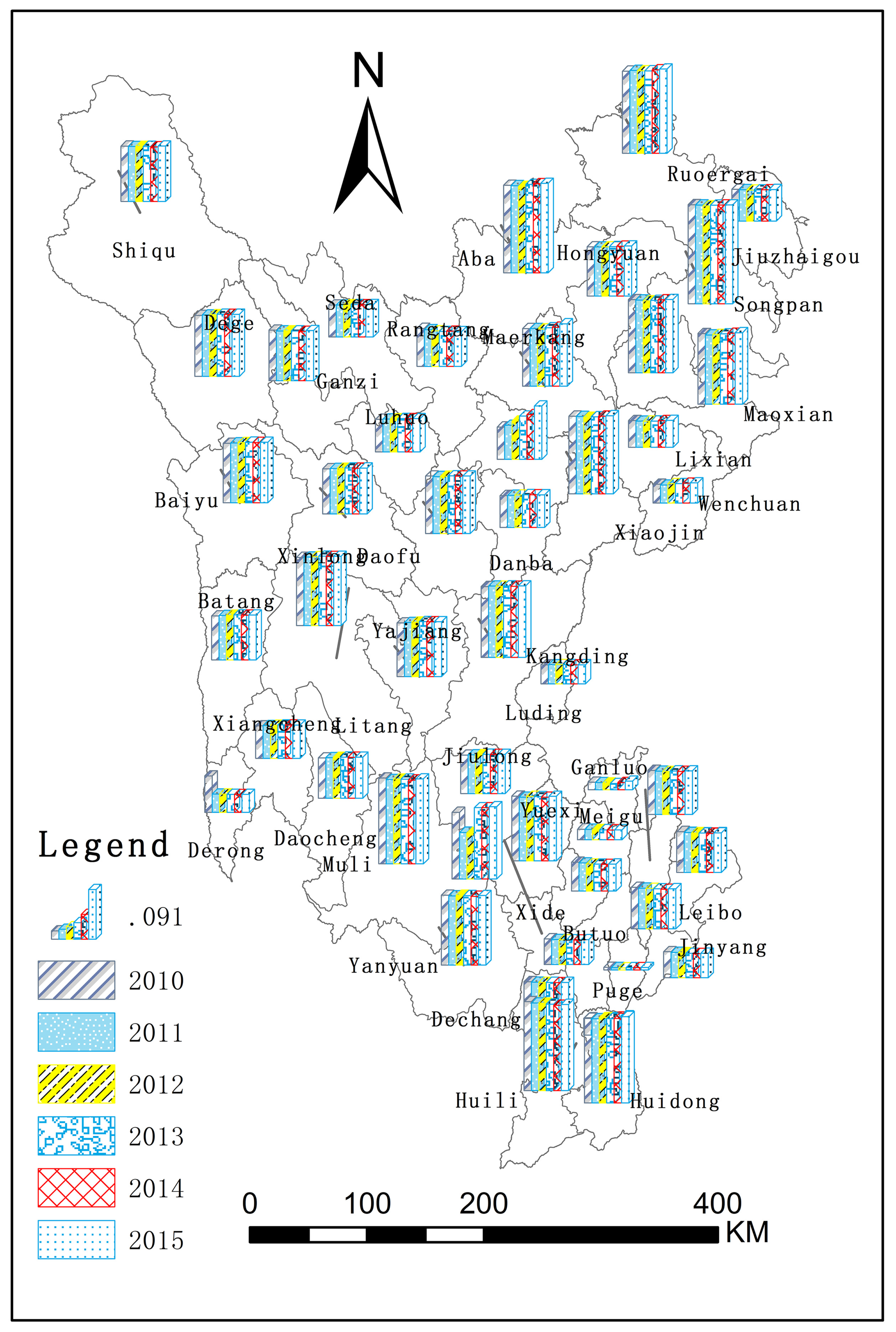
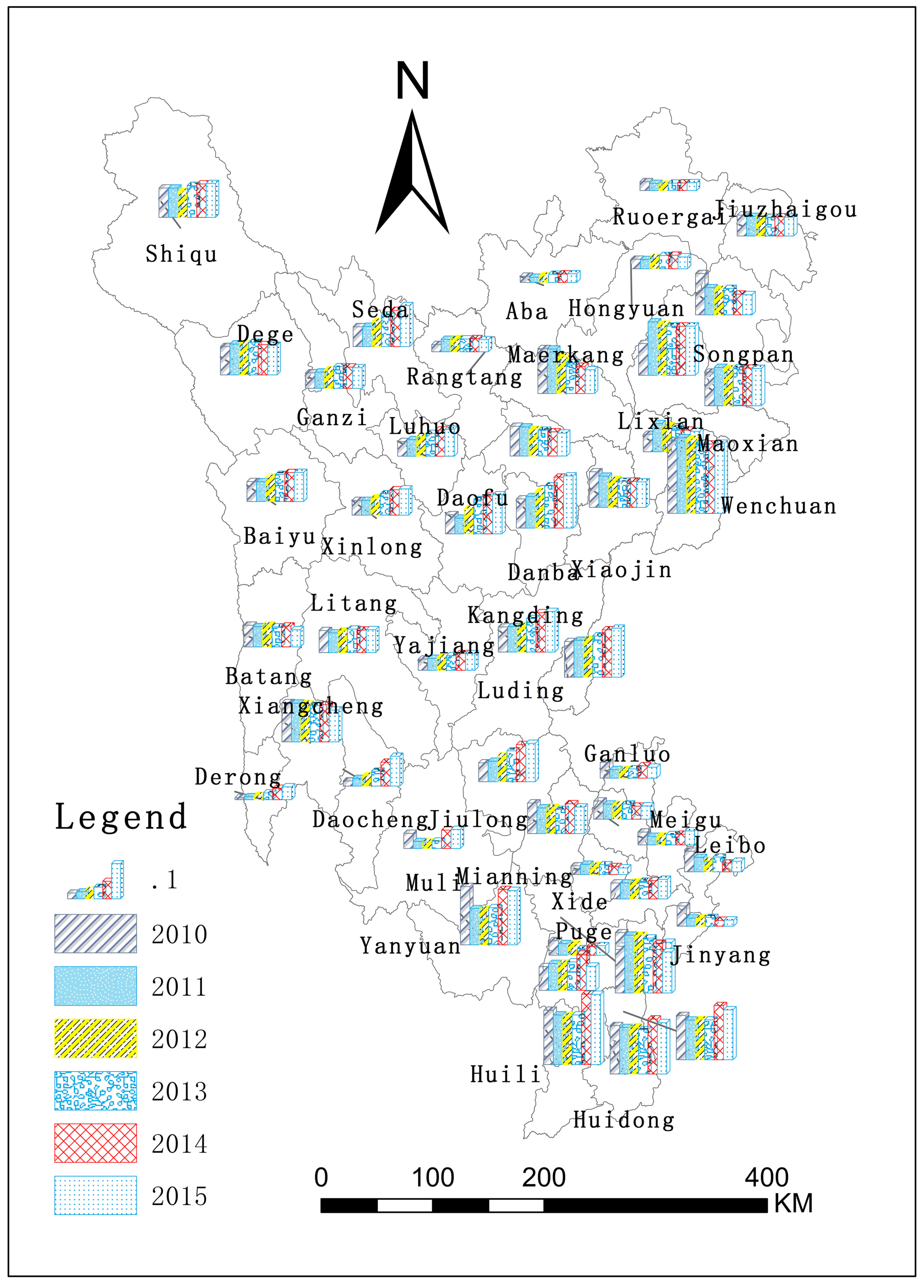
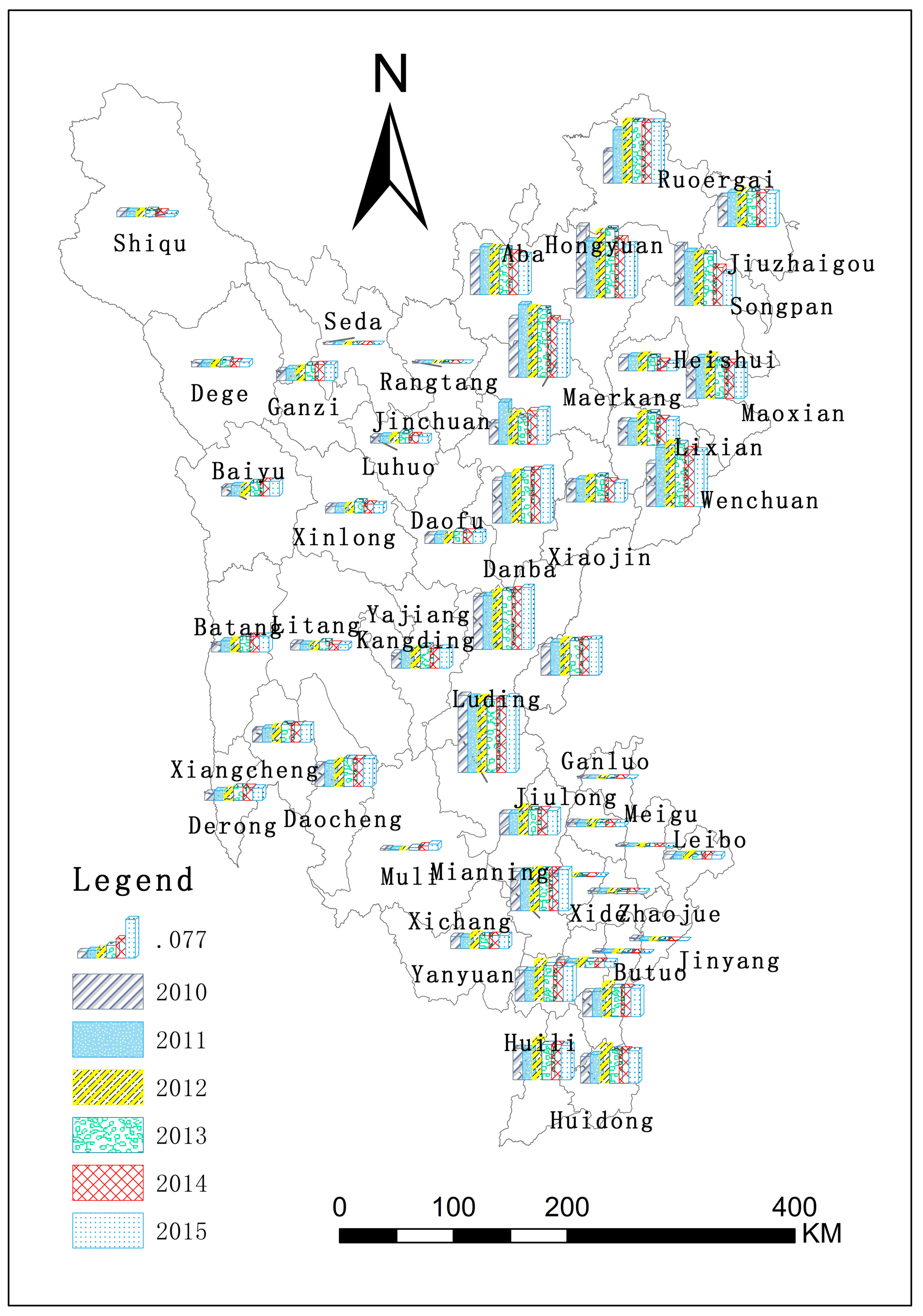
Livelihood capital indicators. This paper refers to related research [34,35,36,37,38] and combines the actual situation of the three states to construct a farmer’s livelihood capital indicator system. Natural capital includes forest land area, grassland area, and cultivated land area. Material capital includes per-capita housing area, number of animals, and rural household electricity consumption. Social capital includes the consumption expenditure of transportation and communication, as well as farmers’ professional cooperative members. Human capital includes the number of labor resources, the number of rural employees, and the number of people trained. Finally, the financial capital includes the per-capita net income of farmers.
(2)
Financial expenditure indicators. The scale of fiscal expenditure is measured by the proportion of regional fiscal expenditure to GDP. At the same time, according to the specific classification criteria of fiscal expenditure in the three-state statistical yearbooks, and also taking into account the uniformity and data availability of fiscal expenditure structure indicators in 47 counties in the study area from 2010 to 2015, the fiscal expenditure is divided into five types: general public service expenditures, agriculture and forestry water expenditures, education expenditures, social security and employment expenditures, and medical expenditures. Moreover, the proportion of various expenditures to the total fiscal expenditure is calculated to measure the structure of fiscal expenditure.
(3)
Other indicators. For the control variables in the model, the regional economic level is measured by the county’s per-capita GDP and the total investment of social fixed assets. The regional social status is measured by the proportion of the county’s minority population. The regional traffic conditions are measured by the county road mileage. The regional ecological environment is measured by ecosystem vulnerability and ecological importance. Regional topographic conditions are measured by altitude, slope, and topographic relief. Finally, regional disaster conditions are measured by the risk of natural disasters.

2.3.2. Calculation Method of Livelihood Capital Level

This paper employs the entropy method [39] to measure the natural capital, physical capital, financial capital, human capital, social capital, and total living capital. Firstly, the original data was standardized; then, the entropy method was used to determine the index weight according to the utility value of each index information; and, finally, the average model was constructed to measure the subsistence capital/total subsistence capital level.

2.3.3. Econometric Model Setting: Dynamic Panel Data Model

This paper cannot take into account all explanatory variables that affect the explained variables, and it is inevitable that missing important variables will lead to bias in the estimation results. Therefore, this paper developed the system Gaussian mixed model (GMM) with reference to the tool variable method used in related research [40] to overcome the bias caused by the endogenous problem of explanatory variables.
The dynamic panel model of the impact of fiscal expenditure scale on farmers’ livelihood capital (Model 1–Model 12) is given as follows:
L n Y i t = α 0 + α 1 L n Y i t 1 + α 2 L n scale i t + α i L n μ i t + ε i t
where Y i t 1 represents the total amount of livelihood capital, natural capital, human capital, financial capital, physical capital, or social capital in the t-1th year of the i-th county.
Furthermore, the dynamic panel model of the impact of fiscal expenditure structure on farmers’ livelihood capital (Model 13–Model 24) is given as follows:
L n Y i t = β 0 + β 1 L n Y i t 1 + β 2 L n s e r v + β 3 L n a g r i + β 4 L n e d u + β 5 L n s o c i + β 6 L n m e d i + β i L n μ i t + ε i t

3. Results

3.1. Descriptive Statistics

3.1.1. Livelihood Capital Level

This paper used the entropy method to calculate the livelihood capital level of the three states from 2010 to 2015 (Figure 4, Figure 5, Figure 6, Figure 7, Figure 8 and Figure 9). From 2010 to 2015, the average stock of human capital is the highest, followed by physical capital, natural capital, and finally, financial capital and social capital. For the total amount of livelihood capital, some counties (cities) have higher level than the average level of the three states in 2010–2015, including Xichang City, Yanyuan County, Huili County, Huidong County, Suining County of Liangshan Prefecture, Wenchuan County, Mao County, Songpan County County, Xiaojin County, Heishui County, Ruoergai County of Aba Prefecture, and Kangding County, Luding County, Danba County, Jiulong County, Dege County, and Shiqu County of Ganzi Prefecture.

3.1.2. Scale and Structure of Fiscal Expenditure

In terms of the scale of fiscal expenditure, the absolute scale of fiscal expenditures in the three states has shown an upward trend year by year, and the proportion of fiscal expenditure to GDP also rises. In terms of the fiscal expenditure structure, during the period between 2010 to 2015, the proportion of general public service expenditures in the three states showed a downward trend as a whole; and the proportion of agriculture and forestry water expenditures in the three states showed an upward trend year by year and was at a high level. Furthermore, although the proportion of educational expenditure showed a trend of fluctuation, it generally showed an increasing trend, and the proportion of expenditure was at a high level. The proportion of social security and employment expenditure in the three states decreases year by year, and the proportion is low. Finally, the proportion of medical and health expenditure in the three states shows an upward trend, but the proportion of medical and health expenditure was at a lower level than the proportion of agriculture and forestry water expenditure, and education expenditure.

3.2. Econometric Model Results

3.2.1. Unit Root Test and Co-Integration Test of Panel Data

(1)
Unit root test. Although the panel data reflect the information in the section, there are still time-series data. The panel data also have the possibility of a unit root. In this paper, the LLC test, IPS test, Fisher–ADF test, and Fisher–PP test were used to conduct unit root tests for explained variables and explanatory variables. If the panel data pass three or more of the four methods, the panel data are stable. The specific test results are as follows:
As can be seen from Table 1, the test results of the four methods show that the unit root exists at the level of human capital (H), physical capital (S), the proportion of total fiscal expenditure to GDP (scale), and general public service expenditure (serv). There was no unit root for other variables, and the first-order difference for the above variables was further carried out. The results show that the first-order difference values were stable at the significance level of 5%. Therefore, the above variable indicators can be used for panel analysis.
(2)
Cointegration test. After confirming that variable indexes can be used for panel analysis, the KAO test method was adopted to conduct a co-integration test of panel data. The test results are as follows:
As can be seen from the Table 2, the adjoint probability value is 0.0000, less than 0.05, indicating that all statistics reject the assumption that there is no co-integration relationship. Thus, there is a co-integration relationship between panel data variables.

3.2.2. The Impact of the Fiscal Expenditure Scale on Livelihood Capital

(1)
Panel model selection test. Firstly, the Hausman test was used to determine whether the random effect model or the fixed effect model should be used. Assuming that there was a random effect in the model, and the original hypothesis would be accepted if the p-value was greater than 0.05: “the random effect is not related to explanatory variables”. The test results are as Table 3:
Table 4 shows the results of the dynamic model using the system GMM, which is a regression using instrumental variables. Model 1, Model 3, Model 5, Model 7, Model 9, and Model 11 are the results of adding only the focus variables (fiscal expenditure scale) and instrumental variables. Model 2, Model 4, Model 6, Model 8, Model 10, and Model 12 are the results of adding focus variables, instrument variables, and control variables. From the AR(2)p-Value, there was no secondary sequence correlation in the generalized gap of the system. From the values of Sarganχ2 (d) and Sargan P, the generalized gap of the system had no over-identification problem. The selected instrumental variables were reasonable, and the estimation results were relatively more accurate. Based on the above description, this paper will analyze the results of the system GMM estimation.
From the AR(2)p-Value, there was no secondary sequence correlation in the generalized gap of the system. From the values of Sargan χ2(d) and Sargan P, the system generalized gap had no over-identification problem. The selected instrumental variables were reasonable, and the estimation results were relatively more accurate. This paper analyzes the system GMM estimation results.
In terms of the relationship between the scale of fiscal expenditure and the level of the livelihood capital of farmers, the total scale of fiscal expenditure had a positive effect on the total stock of livelihood capital at a significant level of 10% and had significant positive effects on natural capital, human capital, financial capital, and physical capital. Among them, the significance and coefficient of the role of financial capital are the largest.
In terms of the relationship between the control variables and the household livelihood capital, per-capita GDP has a significant effect on the total stock of livelihood capital and the remainder of the livelihood capital (except for the social capital), and has a significant negative effect on natural capital. The investment in fixed assets of the whole society has a positive impact on the total amount of livelihood capital, human capital, and financial capital, and has a negative effect on natural capital. The proportion of the ethnic minority population has a negative effect on the total level of livelihood capital, human capital, and financial capital at a significant level of 5%, and has a positive effect on natural capital and physical capital at a significant level of 1%. Furthermore, highway mileage has a significant positive effect on total livelihood capital, human capital, financial capital, and physical capital, and has a negative impact on natural capital.

3.2.3. The Impact of Fiscal Expenditure Structure on Livelihood Capital

(1)
Panel model selection test. Firstly, the Hausman test was used to determine whether the random effect panel data model or the fixed effect panel data model should be established. When P was more than 0.05, the random effect model was generally adopted. Otherwise, the fixed-effect model was adopted. The test results are as Table 5:
Table 6 shows the results of the dynamic model using the system GMM, which is a regression using instrumental variables. Model 13, Model 15, Model 17, Model 19, Model 21, and Model 23 are the results of adding only the focus variables (financial expenditure structure) and instrumental variables. Model 14, Model 16, Model 18, Model 20, Model 22, and Model 24 are the results of adding focus variables, instrument variables, and control variables. From the AR(2)p-value, it can be seen that there is no secondary sequence correlation in the system GMM. From the values of Sarganχ2 (d) and Sargan P, the system GMM has no over-identification problem, and the selected tool variables are more reasonable. This paper will analyze the system GMM estimation results.
In terms of the relationship between the scale of fiscal expenditure and the level of livelihood capital of farmers, general public service expenditure had a negative effect on the total amount of livelihood capital, natural capital, and financial capital. Agriculture and forestry water expenditures had a positive effect on total livelihood capital, natural capital, financial capital, physical capital, and social capital. Among them, the coefficient of influence on natural capital was the largest, but had no significant effect on human capital. Educational expenditure had a positive effect on the total amount of livelihood capital, human capital, financial capital, and social capital, and had a negative effect on natural capital. Specifically, educational expenditure had the most significant effect on human capital. Together, social security and employment expenditure, and medical expenditure had positive effects on total livelihood capital, human capital, and financial capital; and had a negative impact on natural capital, with the greatest impact on financial capital.
In terms of the relationship between control variables and farmers’ livelihood capital levels, per-capita GDP had a negative effect on natural capital and positive effects on human capital, financial capital, and material capital. The fixed asset investment of the whole society had no effect on physical capital and social capital, but had positive impacts on financial capital and human capital. The proportion of the ethnic minority population has significant negative effects on the total amount of livelihood capital, human capital, and financial capital, and had a positive effect on natural capital and material capital. Moreover, highway mileage had a significant positive effect on total livelihood capital, human capital, and financial capital, and its effect on natural capital was significantly negative.
In general, Hypothesis 1, Hypothesis 2, Hypothesis 4, and Hypothesis 5 were validated, while Hypothesis 3 and Hypothesis 6 were partially validated. The unverified parts are the positive impact of general public service expenditures on financial capital and total capital stocks. Furthermore, the empirical result was the opposite, and the general public service expenditure had negative impacts on the financial capital and the total stock of livelihood capital.

4. Discussion

From 2010 to 2015, the average stock of human capital in the household livelihood capital in the three states was the highest, followed by physical capital, natural capital, and finally financial and social capital. The average financial capital of the three states was low, reflecting that the average income of farmers is not high. The low average value of social capital may be limited by the lack of traffic and communication, the lack of social organization, and the lack of awareness of farmers in participating in public activities.
By analyzing the impact of the fiscal expenditure scale on the livelihood capital, it was found that the total scale of fiscal expenditure has a positive effect on the total stock of livelihood capital at a significant level of 10%, indicating that the scale of fiscal expenditure has a positive effect on the increase in the total amount of the livelihood capital of farmers. Specifically, the scale of fiscal expenditure has a significant positive effect on natural capital, human capital, financial capital, and physical capital. Among them, the significance and coefficient of financial capital were the largest [41], indicating that fiscal expenditure can significantly increase the income of farmers, giving tangible benefits. This significantly helps to improve the livelihood of farmers and thus reduce poverty [42]. In addition to having no impact on social capital, per-capita GDP had a significant effect on the total stock of livelihood capital and the remainder of the livelihood capital. Additionally, it had a significant negative effect on natural capital, indicating that regional economic development means sacrificing certain natural resources but, to a certain extent, promoting the increase of the livelihood capital of farmers. The investment in fixed assets of the whole society had a positive impact on the total amount of livelihood capital, human capital and financial capital, and had a negative effect on natural capital. The fixed asset investment in the whole society was conducive to enhancing economic strength, increasing employment channels and improving the livelihood level of farmers. However, the increase in fixed asset investment in the whole society also means an increase in demand for construction land and a reduction in natural capital. The proportion of the ethnic minority population has a negative impact on the total level of livelihood capital, human capital, and financial capital at a significant level of 5%. Furthermore, it has a positive effect on natural capital and physical capital at a significant level of 1%. The agglomeration area of the ethnic minority population was less educated. The ideas and attitudes of people in these areas were relatively conservative and closed. It was difficult to go out for work, and the skills for earning a living were minimal. These factors combined resulted in a low level of non-agricultural activities and a low total stock of household livelihood capital. Additionally, highway mileage had a significant positive effect on total livelihood capital, human capital, financial capital, and physical capital, and had a negative impact on natural capital. The higher the highway mileage, the better the traffic conditions. The improvement of traffic conditions has brought about an increase in the level of household livelihood capital. At the same time, the higher the mileage on highways, the more arable land resources are occupied by the infrastructure construction related to road construction, resulting in lower natural capital levels for farmers.
By analyzing the impact of fiscal expenditure structure on livelihood capital, it is revealed that general public service expenditure has a negative effect on total livelihood capital, natural capital and financial capital. Therefore, the government should establish an efficient fiscal expenditure system.
Agriculture, forestry and water expenditures have a positive effect on total livelihood capital, natural capital, financial capital, physical capital and social capital. Scholars’ research also confirmed this view. Therefore, they proposed that the government should strengthen financial expenditure on social security and employment, science and technology, education, agriculture, forestry and water [43,44]. Among them, the coefficient of influence on natural capital was the largest but had no significant effect on human capital. Educational expenditure had a positive effect on the total amount of livelihood capital, human capital, financial capital, and social capital, and had a negative effect on natural capital. Specifically, education expenditure has the most significant effect on human capital. Furthermore, social security, employment expenditure, and medical expenditure all have positive effects on total livelihood capital, human capital, and financial capital; and have a negative impact on natural capital, with the greatest impact on financial capital. Additionally, the impact of education expenditure on each livelihood capital is greater than the impact of social security and employment expenditure, and medical expenditure on each livelihood capital. The results of the impact directions of per-capita GDP, total social fixed asset investment, minority population, and highway mileage on the livelihood capital are basically the same as the fiscal expenditure scale on livelihood capital.

5. Conclusions and Policy Implications

5.1. Conclusions

In this study, the entropy method was used to calculate the stock of each livelihood capital, and an in-depth analysis was carried out. Based on the calculations, the impact of the scale and structure of fiscal expenditure on livelihood capital is discussed. The conclusions of these findings are as follows:
(1)
Characteristics of livelihood capital: From 2010 to 2015, the average stock of human capital in the three states was the highest during the livelihood capital composition, followed by physical capital, natural capital, and finally, financial capital and social capital;
(2)
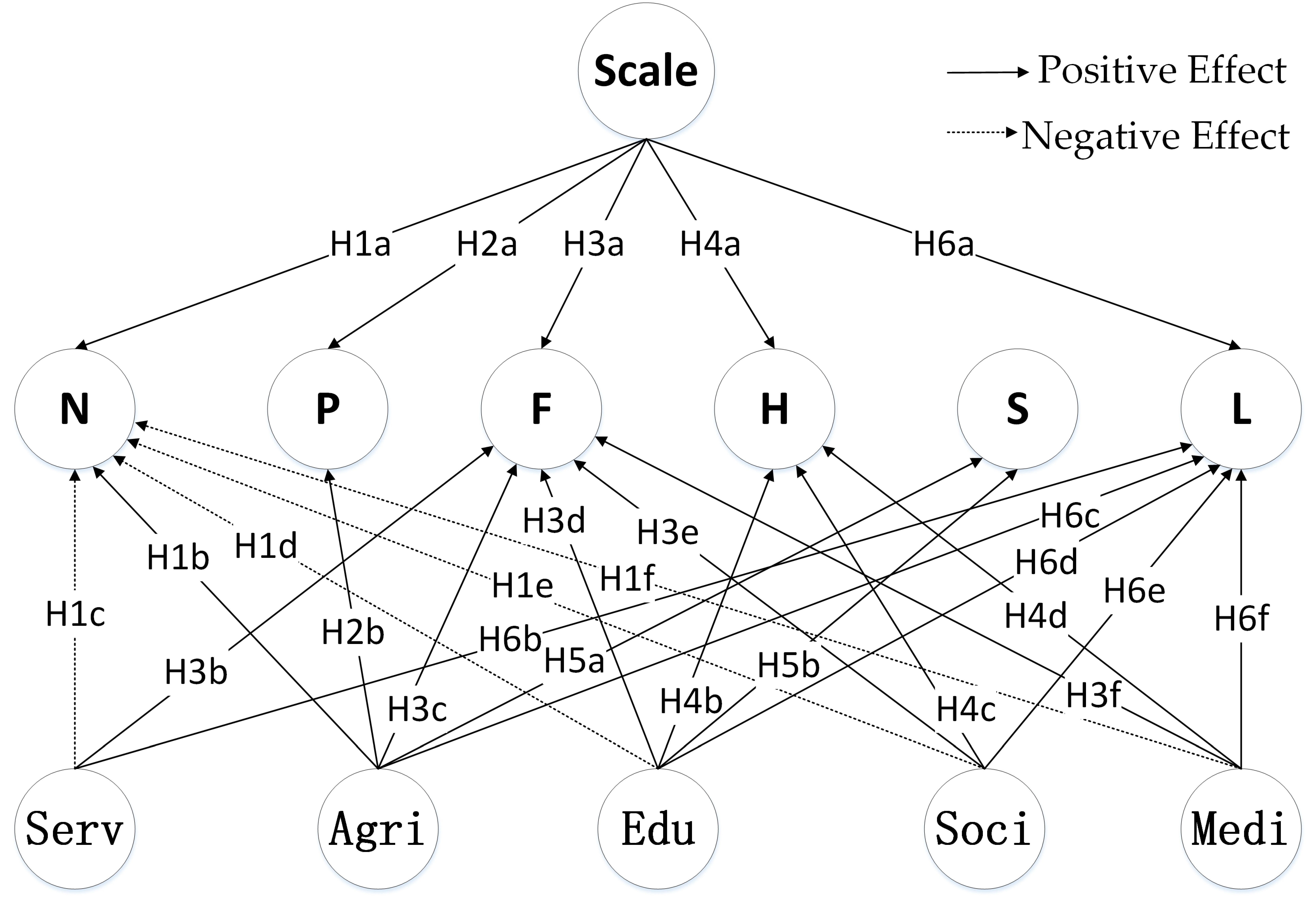
Natural capital and physical capital were positively affected by the total scale of fiscal expenditure, agriculture, forestry, and water expenditure, and the former was negatively affected by general public service expenditure, education expenditure, social security and employment expenditure, and medical expenditure;
(3)
Financial capital and the total amount of livelihood capital were positively affected by the total scale of fiscal expenditure, agriculture, forestry and water expenditure, education expenditure, social security and employment expenditure, and medical expenditure, and negatively affected by general public service expenditure;
(4)
Human capital was positively affected by the total scale of fiscal expenditure, education expenditure, social security and employment expenditure, and medical expenditure;
(5)
Social capital was positively affected by agriculture, forestry and water expenditure, and education expenditure.

5.2. Policy Implications

The majority of China’s mountainous areas are ethnic minority communities and concentrated contiguous poverty-stricken areas. The sustainable livelihood of farmers is the micro-foundation for precise poverty alleviation. The research on the impact of the fiscal expenditures on the livelihood capital of farmers across Liangshan Prefecture, Ganzi Prefecture and Aba Prefecture serves to provide a scientific basis for the in-depth study of farmers’ sustainable livelihood. Based on the above research results, the following countermeasures are proposed:
First, the scale of fiscal expenditures should be reasonably increased. Since the impact of different fiscal expenditure items on the respective livelihood capital is not the same, the scale of fiscal expenditures for each purpose can be adjusted in a targeted manner, and key fiscal expenditure items should be supported to achieve “no shortage, no offside”. For example, although general public service expenditure is an indispensable part of fiscal expenditure, it can be saved when there is no significant impact on livelihood capital so that more fiscal expenditures can be used optimally.
Second, the scale and proportion of agriculture, forestry and water expenditures, education expenditures, social security and employment expenditures, and medical expenditures should be realistically increased. Expenditure on science, education, culture, and health has a basic and long-term promotion effect on social and human capital, as well as technological development. These factors have also been confirmed through the endogenous economic growth theory as an important determinant of economic development. Therefore, appropriate increases in education expenditure, social security and employment expenditures, and medical expenditures have played a positive role in increasing farmers’ income, improving the social security system, and promoting improvements in science and technology. Additionally, this study reveals that the impact coefficient of education expenditure is greater than social security and employment expenditure, and medical expenditure. This is mainly due to the fact that education expenditure is a fundamental policy. In areas where ethnic minorities are concentrated, the level of education is underdeveloped, and there is a situation in which poverty can easily relapse into even more devastating poverty. Education is conducive to improving the ability of farmers to become self-reliant. Therefore, on the basis of increasing social expenditures, it is necessary to further increase the scale and proportion of education expenditure.
Third, traffic conditions and achievement in information and resource sharing should be optimized. Liangshan Prefecture, Ganzi Prefecture, and Aba Prefecture are typical mountainous areas. Although natural resources are abundant, infrastructure is inadequate and traffic conditions are poor, which hinders economic exchanges and resource exchanges with the outside world. This study reveals that highway mileage has a significant positive effect on the total amount of livelihood capital, human capital, and financial capital. Specifically, the quality of the traffic conditions determines the level of household livelihood capital to a certain extent and verifies that “to be rich, is to repair the roads first”. Therefore, it is necessary to increase infrastructure construction and optimize traffic conditions to achieve sustainable development.

Author Contributions

Conceptualization, S.G., B.W., K.Z. and Q.Z.; methodology, S.G., D.X., H.W., and K.Z.; software, S.G., B.W., K.Z., and Q.Z.; validation, Q.Z., D.X. and H.W.; formal analysis, S.G., D.X.; investigation, B.W., K.Z., and Q.Z.; resources, S.G., B.W. and K.Z.; data curation, S.G. and D.X.; writing—original draft preparation, S.G., B.W., K.Z., D.X., H.W. and Q.Z.; writing—review and editing, S.G., B.W. and K.Z.; visualization, S.G., B.W. and K.Z.; supervision, Q.Z., D.X. and H.W.; project administration, B.W., K.Z.; funding acquisition, S.G., D.X., H.W. and K.Z. All authors have read and agreed to the published version of the manuscript.

Funding

This research received funding from Sichuan Province Social Science Research “14th Five-Year Plan” 2021 Annual Project (SC21ST011), the Fundamental Research Funds for the Central Universities (JBK2102018), the National Natural Science Foundation of China (Grant No. 41601614) and the Sichuan Center for Rural Development Research (CR2107).

Institutional Review Board Statement

Not applicable.

Informed Consent Statement

Informed consent was obtained from all subjects involved in the study.

Data Availability Statement

Not applicable.

Conflicts of Interest

The authors declare no conflict of interest.

References

  1. Cui, P. Progress in Research on Mountain Diasters in China and Scientific Issues to Be Concerned in the Future. Prog. Geogr. 2010, 33, 145–152. [Google Scholar] [CrossRef]
  2. Chen, G.J.; Fang, Y.P.; Chen, Y. China Mountain Development Report—Research on Mountain Settlement in China; The Commercial Press: Beijing, China, 2007. [Google Scholar]
  3. Su, F.; Shang, H.Y. The Impact of Farmers’ Livelihood Capital on Their Risk Coping Strategies: Taking Zhangye City in the Heihe River Basin as an Example. China Rural. Econ. 2012, 8, 79–87. [Google Scholar]
  4. Xin, G.X.; Yan, J.Z.; Yang, Q.Y. The Changes of Rural Households’ Living Life and Their Livelihood Transformation in New Rural Construction. J. Southwest Univ. 2012, 34, 122–130. [Google Scholar] [CrossRef]
  5. Su, F.; Pu, X.D. Research on the relationship between livelihood capital and livelihood strategy. China Popul. Resour. Environ. 2009, 6, 119–124. [Google Scholar]
  6. Liu, C.F.; Liu, Y.Y.; Wang, C. Characteristics and Influencing Factors of Livelihood Capital of Poor Farmers in Loess Hilly Region: Taking Suizhong County of Gansu Province as an Example. Econ. Geogr. 2017, 37, 153–162. [Google Scholar] [CrossRef]
  7. Kenneth, J.A.; Mordecai, K. Optimal growth with irreversible investment in a Ramsey model. Econom. J. Econom. Soc. 1970, 38, 331–344. [Google Scholar] [CrossRef]
  8. Barro, R.J. Government Spending in A Simple Model of Endogenous Growth. J. Political Econ. 1990, 98, S103–S125. [Google Scholar] [CrossRef] [Green Version]
  9. Gong, L.T.; Zou, H.Y. The impact of government public spending growth and volatility on economic growth. Foreign Econ. Theory Rev. 2001, 9, 58–63. [Google Scholar]
  10. Helms, L.J. The effect of State and Local Taxes on Economics Growth, A Time Series—Cross Section Approach. Rev. Econ. Stat. 1985, 67, 574–582. [Google Scholar] [CrossRef]
  11. Easterly, R. Fiscal Policy and Economic Growth, An Empirical Investigation. J. Monet. Econ. 1993, 32, 417–458. [Google Scholar] [CrossRef]
  12. Cai, Z.Z. An Econometric Analysis of the Contribution of Education to Economic Growth: An Empirical Basis of the Strategy of Rejuvenating the Country through Science and Education. Econ. Res. 1999, 2, 40–48. [Google Scholar]
  13. Cai, Z.H. Analysis of Livelihood Capital of Farmers in Poor Villages in Wenchuan Earthquake Area. China Rural. Econ. 2010, 12, 55–67. [Google Scholar]
  14. He, R.W.; Liu, S.Q.; Liu, Y.W. Evaluation of livelihood capital of typical mountain farmers and its spatial pattern: Taking Liangshan Yi Autonomous Prefecture in Sichuan Province as an example. J. Mt. Res. 2014, 32, 641–651. [Google Scholar] [CrossRef]
  15. Nawrotzki, J.R.; Huntrer, M.L.; Dickinson, W.T. Rural livelihood and access to natural capitals: Differences between migrants and non-migrants in Madagascar. Demogr. Res. 2012, 26, 661–700. [Google Scholar] [CrossRef] [PubMed] [Green Version]
  16. Cui, S.Y.; Xu, D.D.; Peng, L.; Liu, S.Q. Characteristics and Differences of Subsistence Immigrants and Aboriginal Livelihood Capital in the Three Gorges Reservoir Area: Taking Wanzhou District of Chongqing as an Example. J. Southwest China Norm. Univ. (Nat. Sci. Ed.) 2016, 4, 80–86. [Google Scholar] [CrossRef]
  17. Xu, D.D.; Zhang, J.F.; Rasul, G.; Liu, S.Q.; Xie, F.T.; Cao, M.T. Household livelihood strategies and dependence on agriculture in the mountainous settlements in the Three Gorges reservoir area, China. Sustainability 2015, 7, 4850–4869. [Google Scholar] [CrossRef] [Green Version]
  18. Ellis, F. Rural Livelihoods and Diversity in Developing Countries; Oxford University Press: New York, NY, USA, 2000. [Google Scholar]
  19. Noelia, Z.C.; Raquel, M.P. Exploring local people’s views on the livelihood impacts of privately versus community managed conservation strategies in the Ruvuma landscape of North Mozambique-South Tanzania. J. Environ. Manag. 2017, 11, 853–862. [Google Scholar] [CrossRef]
  20. Du, Y.H.; Huang, X.Z. Research on the relationship between financial capital agricultural expenditure and farmers’ income. Stat. Res. 2006, 9, 47–50. [Google Scholar] [CrossRef]
  21. Li, H.Z.; Qian, Z.H. Financial Supporting Agriculture Policy and Agricultural Growth in China, Analysis of Causality and Structure. China Rural. Econ. 2004, 8, 38–43. [Google Scholar]
  22. Liu, H. An empirical analysis of the impact of fiscal support for agriculture on agricultural economic growth. Agric. Econ. Issues 2008, 10, 30–35. [Google Scholar] [CrossRef]
  23. Meng, Z.X.; Meng, H.S. An Empirical Study on the Relationship between Financial Expenditure and Farmers’ Income in Shanxi Province. China Urban Econ. 2011, 3. [Google Scholar]
  24. Wang, H.Y.; Meng, Q.S.; Yan, H.S.; Tang, K. Research on the Relationship between Fiscal Agricultural Expenditure and Peasant Income Growth. J. Northwest A&F Univ. (Soc. Sci. Ed.) 2014, 14, 72–79. [Google Scholar] [CrossRef]
  25. Yang, C.M. An Empirical Analysis of the Sources of Farmers’ Income in China: Also on the Countermeasures to Increase Farmers’ Income. Financ. Trade Econ. 2007, 2. [Google Scholar]
  26. Xiong, J.F.; Ding, S.J. Invalidity test of the impact of “NRCMS” on farmers’ livelihood strategies. Econ. Issues 2010, 1, 15–22. [Google Scholar] [CrossRef]
  27. Wang, M.; Pan, Y.H. Research on the relationship between fiscal agricultural investment and farmers’ net income. Agric. Econ. Issues 2007, 5, 99–105. [Google Scholar] [CrossRef]
  28. Yan, C.L.; Gong, L.T. Financial expenditure, tax expenditure, taxation and long-term economic growth. Econ. Res. 2009, 6. [Google Scholar]
  29. Xie, X.X.; Zhang, S.Q.; Zhu, S.T. Effects of Returning Farmland to Forests on Sustainable Livelihood of Farmers. J. Peking Univ. (Nat. Sci.) 2010, 46, 457–464. [Google Scholar] [CrossRef]
  30. Zhu, Y.C. Research on the income distribution effect of China’s financial support for agriculture. Contemp. Financ. Econ. 2013, 9, 39–48. [Google Scholar]
  31. Luo, D.; Jiao, J. Empirical study on the impact of national financial support for farmers on farmers’ income. Agric. Econ. Issues 2014, 12, 48–53. [Google Scholar] [CrossRef]
  32. Li, C.; Liu, W.; Huang, Q. Analysis of the Status Quo and Influencing Factors of Farmers’ Livelihood Capital in the Background of Relocation of Southern Shaanxi Immigrants. Contemp. Econ. Sci. 2014, 36, 106–126. [Google Scholar] [CrossRef]
  33. Huang, X.Z.; Wang, H.L. On the Performance of China’s Financial Supporting Agriculture Funds from the Perspective of Increasing Farmers’ Income. J. Cent. Univ. Financ. Econ. 2005, 1, 10–13. [Google Scholar] [CrossRef]
  34. Shui, W.; Bai, J.P.; Zhang, S. Analysis of the influencing factors on resettled farmer’s satisfaction under the policy of the balance between urban construction land increasing and rural construction land decreasing. Sustainability 2014, 6, 8522–8535. [Google Scholar] [CrossRef] [Green Version]
  35. Fearnside, P.M. Challenges for sustainable development in Brazilian Amazonia. Sustain. Dev. 2018, 26, 141–149. [Google Scholar] [CrossRef]
  36. Asongu, S.A.; Odhiambo, N.M. Environmental degradation and inclusive human development in sub-Saharan Africa. Sustain. Dev. 2019, 27, 25–34. [Google Scholar] [CrossRef] [Green Version]
  37. Lan, X.; Weng, L.F.; Yu, H.Z. Addressing policy challenges in implementing Sustainable Development Goals through an adaptive governance approach: A view from transitional China. Sustain. Dev. 2018, 26, 150–158. [Google Scholar] [CrossRef]
  38. Nölting, B.; Mann, C. Governance strategy for sustainable land management and water reuse: Challenges for transdisciplinary research. Sustain. Dev. 2018, 26, 691–700. [Google Scholar] [CrossRef]
  39. Zhang, W.M. Evaluation Model of Urban Sustainable Development Based on Entropy Method. J. Xiamen Univ. (Philos. Soc. Sci.) 2004, 2, 109–115. [Google Scholar] [CrossRef]
  40. Shao, X.K.; Hu, H.G. Endogenous in the empirical study of economic growth. China Popul. Resour. Environ. 2015, 3, 109–118. [Google Scholar]
  41. Liu, J. The impact of sustainable livelihood capital on Farmers’ Income: An Empirical Study Based on information entropy method. Stat. Decis. Mak. 2012, 17, 103–105. [Google Scholar]
  42. Xu, D.D.; Peng, L.; Liu, S.Q.; Chen, T.T. Influences of migrant work income on the poverty vulnerability disaster threatened area, A case study of the Three Gorges Reservoir area, China. Int. J. Disaster Risk Reduct. 2017, 22, 62–70. [Google Scholar] [CrossRef]
  43. Zhang, Y. Research on the realization path of financial support for farmers’ sustainable livelihood in the Lijiang River Basin. Mod. Mark. 2020, 5, 48–49. [Google Scholar]
  44. Ye, H. Analysis on the impact of public finance policy on Farmers’ income under the framework of livelihood capital—Based on the survey of two minority poor counties in Chongqing. J. Cent. South Univ. Natl. (Humanit. Soc. Sci.) 2015, 35, 114–119. [Google Scholar]
Figure 1. Research framework.
Agriculture 12 00881 g001
Figure 2. Research Hypotheses.
Agriculture 12 00881 g002
Figure 3. Location of study region.
Agriculture 12 00881 g003
Figure 4. Natural capital level.
Agriculture 12 00881 g004
Figure 5. Physical capital level.
Agriculture 12 00881 g005
Figure 6. Financial capital level.
Agriculture 12 00881 g006
Figure 7. Human capital level.
Agriculture 12 00881 g007
Figure 8. Social capital level.
Agriculture 12 00881 g008
Figure 9. The total amount of livelihood capital.
Agriculture 12 00881 g009
Table 1. Results of unit root test.
VariableLLC InspectionIPS InspectionFisher-ADF InspectionFisher-PP InspectionConclusion
StatisticProb.StatisticProb.StatisticProb.StatisticProb.
Ln(L)−58.22280.0000−8.11720.0000169.8860.0000240.7320.0000smooth
Ln(N)−10.83090.0000−1.96930.0000139.4980.0010221.0140.0000smooth
Ln(H)−9.49030.00001.02790.848091.65640.4316148.3490.0001unsmooth
Ln(F)−20.92300.0000−4.37540.0000166.3550.0000256.9270.0000smooth
Ln(P)−15.78340.0000−3.14710.0008136.7900.0026157.7680.0000smooth
Ln(S)−4.25730.0000−0.43740.3309118.3050.0338159.5440.0000unsmooth
Ln(scale)−6.48860.0000−1.25720.1043135.1380.0035176.2090.0000unsmooth
Ln(serv)−1.00020.15862.50640.993979.29890.860996.60320.4065unsmooth
Ln(agri)−26.82210.0000−7.04390.0000217.4990.0000263.7650.0000smooth
Ln(edu)−15.66410.0000−2.54130.0055132.7980.0052152.0800.0001smooth
Ln(soci)−13.85340.0000−2.64240.0041145.9340.0005212.4450.0000smooth
Ln(medi)−31.53770.0000−6.34570.0000199.3400.0000250.6170.0000smooth
D(Ln(H))−13.72700.0000−3.56900.0002118.4330.0239145.3530.0002smooth
D(Ln(S))−20.52570.0000−8.31960.0000191.7130.0000231.6480.0000smooth
D(Ln(scale))−32.27140.0000−11.17130.0000236.6070.0000253.6700.0000smooth
D(Ln(serv))−26.64540.0000−7.13660.0000159.8540.0000175.6120.0000smooth
D(X1)−18.13610.0000−8.26380.0000182.6870.0000217.0280.0000smooth
D is the first difference.
Table 2. Co-integration test results.
Inspection MethodsStatistics ofStatistical Quantityp-Values
KAO inspectionADF−4.10440.0000
Table 3. Hausman test results.
Dependent VariableChi-Sq. Statisticp-ValuesSelect the Model
Ln(L)14.51170.0127Fixed effect model
Ln(N)6.60730.2515Stochastic effect model
Ln(H)9.82780.0803Stochastic effect model
Ln(F)21.98660.0005Fixed effect model
Ln(P)14.26570.0140Fixed effect model
Ln(S)13.79520.0170Fixed effect model
Table 4. The dynamics regression model result of the impact of the fiscal expenditure scale on livelihood capital.
VariablesTotal Livelihood CapitalNatural CapitalHuman CapitalFinancial CapitalPhysical CapitalSocial Capital
Model 1Model 2Model 3Model 4Model 5Model 6Model 7Model 8Model 9Model 10Model 11Model 12
Ln(L(−1))0.900 ***
(−43.32)
0.748 ***
(14.94)
Ln(N(−1)) 0.360 ***
(−41.54)
0.299 ***
(−15.52)
Ln(H(−1)) −0.138 ***
(−25.88)
−0.26 ***
(−17.82)
Ln(F(−1)) 0.741 ***
(−31.54)
0.820 ***
(−21.36)
Ln(P(−1)) 0.862 ***
(−18.56)
1.058 ***
(−12.18)
Ln(S(−1)0 0.812 ***
(−33)
0.658 ***
(−21.17)
Ln(Scale)0.025 *
(−1.78)
0.010 *
(−0.3)
0.075 ***
(−11.57)
0.038 ***
(−3.55)
0.294 ***
(−4.47)
0.02 ***
(−0.36)
0.359 ***
(−4.03)
0.323 **
(−1.21)
0.080 ***
(−4.62)
0.039 **
(−1.81)
−0.198
(−4.20)
0.101
(−2.22)
Ln(Pergdp) 0.071 ***
(1.51)
−0.074 **
(−2.33)
0.85 ***
(−4.37)
0.217 ***
(−1.1)
0.102 **
(−0.87)
0.243
(−1)
Ln(Invest) 0.014 *
(−0.91)
−0.057 *
(−4.14)
0.21 ***
(−3.47)
0.107 *
(−1.73)
−0.048
(−1.33)
0.071
(−0.69)
Ln(Mino) −0.346 **
(−0.71)
0.707 **
(−2.46)
−4.23 **
(−2.52)
−2.08 **
(−2.25)
0.620 ***
(−2.82)
−0.085
(−0.29)
Ln(Way) 0.119 ***
(−2.05)
−0.104 ***
(−3.20)
0.50 *
(−1.86)
0.406 **
(−1.45)
0.087 **
(−2.01)
0.306
(−1.47)
Sarganχ2(d)16.06
(−10)
11.78
(−10)
20.69
(−10)
23.78
(−10)
21.04
(−10)
18.78
(−10)
24.17
(−10)
13.76
(−10)
29.49
(−10)
25.41
(−10)
12.25
(−10)
21.21
(−10)
Sargan P 0.100.300.230.080.210.430.070.180.100.460.270.10
AR(2)P 0.570.390.110.170.310.310.160.160.610.580.600.72
* (1) The value in parentheses is the t-statistics corresponding to the estimated coefficients. *** indicates significance at the 1% level; ** indicates significance at the 5% level; and * indicates significance at the 10% level. (2) Sarganχ2(d) is the Sargan statistic obtained by over-identifying the plausibility of the instrumental variable, and the Sargan p-Value is the corresponding p-Value. (3) The AR(2)P represents the value obtained by performing the second-order sequence correlation test on the residual after the first-order difference, and the original hypothesis is that there is no second-order autocorrelation in the model.
Table 5. Hausman test results.
Dependent VariableChi-Sq. Statisticp-ValuesSelect the Model
Ln(L)44.18140.0000Fixed effect model
Ln(N)15.23920.1236Stochastic effect model
Ln(H)13.88660.1782Stochastic effect model
Ln(F)23.51640.0090Fixed effect model
Ln(P)8.61530.5690Stochastic effect model
Ln(S)11.59760.3129Stochastic effect model
Table 6. The dynamics regression model result of the impact of the fiscal expenditure structure on livelihood capital.
VariablesTotal Livelihood CapitalNatural CapitalHuman CapitalFinancial CapitalPhysical CapitalSocial Capital
Model 13Model 14Model15Model 16Mode l17Model 18Model 19Model 20Model 21Model 22Model 23Model 24
Ln(L(-1))0.901 ***
(−36)
0.758 ***
(−17.72)
Ln(N(-1)) 0.315 ***
(−41.07)
0.267 ***
(−10.23)
Ln(H(-1)) −0.129 ***
(−20.47)
−0.242 ***
(−10.00)
Ln(F(-1)) 0.694 ***
(−64.19)
0.824 ***
(−14.77)
Ln(P(-1)) 0.971 ***
(−21.66)
1.116 ***
(−9.22)
Ln(S(-1) 0.792 ***
(−31.68)
0.660 ***
(−20.59)
Ln(Serv)−0.013 *
(−0.46)
−0.041 *
(−1.12)
−0.069 ***
(−3.42)
−0.108 ***
(−4.55)
−0.112
(−2.17)
0.112
−0.93
−0.627 ***
(−3.93)
−0.483 **
−2.46
0.024
(−0.33)
−0.01
(−0.11)
0.286
−1.19
−0.066
(−0.31)
Ln(Agri)0.116 **
(−0.3)
0.403 **
(−0.77)
0.586 *
(−1.82)
0.663 **
(−2.18)
−0.268
(−3.30)
−0.257
(−1.20)
0.129 **
(−0.67)
0.090 **
(−0.43)
0.078 *
(−0.78)
0.188 **
(−1.78)
0.535 *
(−2.69)
0.481 *
(−1.88)
Ln(Edu)0.115 **
(−0.34)
0.595 **
(−1.43)
−0.097 ***
(−5.27)
−0.117 ***
(−6.49)
0.475 ***
(−4.02)
0.450 ***
(−4.24)
0.072 *
(−0.41)
0.589 **
(−2.1)
−0.13
(−1.68)
−0.091
(−1.22)
0.338 **
(−2.17)
0.326 *
(−1.7)
Ln(Soci)0.101 **
(−0.45)
0.051 *
(−1.21)
−0.017 **
(−2.51)
−0.099 ***
(−3.20)
0.045 ***
(−0.92)
0.101 **
(−0.82)
0.772 **
(−4.08)
0.552 **
(−2.55)
−0.073
(−0.98)
−0.143
(−1.55)
0.58
(−5.77)
0.436
(−3.44)
Ln(Medi)0.027 *
(−0.74)
0.045 *
(−0.95)
−0.067 ***
(−4.56)
−0.147 ***
(−7.76)
0.330 ***
(−3.83)
0.224 **
(−1.26)
0.198 **
(−1.13)
0.252 **
(−1.12)
−0.125
(−1.46)
−0.141
(−1.51)
0.069
(−0.34)
−0.115
(−0.48)
Ln(Pergdp) 0.437 **
(−0.82)
−0.088 ***
(−2.72)
0.543 **
(−2.26)
0.515 **
(−1.93)
0.015 **
(−0.12)
0.006
(−0.02)
Ln(Invest) 0.03
(−2.43)
−0.054 ***
(−4.41)
0.169 **
(−2.25)
0.029 ***
(−0.44)
−0.055
(−1.57)
0.136
(−1.29)
Ln(Mino) −0.111 ***
(−1.16)
0.619
(−1.63)
−0.333 **
(−1.55)
−0.519 **
(−2.03)
0.803 **
(−2.98)
−0.561 **
(−2.04)
Ln(Way) 0.125 *
(−1.72)
−0.208 ***
(−3.81)
0.109 **
(−0.54)
0.052 **
(−0.18)
−0.075
(−1.44)
0.088
(−0.45)
Sarganχ2 (d)11.048 (−10)14.1111 (−10)22.4752 (−10)20.7586 (−10)25.2916 (−10)11.7704 (−10)25.6425 (−10)14.3549 (−10)21.2546 (−10) 12.6974 (−10)20.8281 (−10)
Sargan P0.35380.1680.12910.2280.480.30070.43310.15740.194 0.24110.2231
AR(2)P0.50910.40220.16140.2860.3070.30860.15470.15680.4364 0.57810.6077
* (1) The value in parentheses is the t-statistics corresponding to the estimated coefficients. *** indicates significance at the 1% level; ** indicates significance at the 5% level; and * indicates significance at the 10% level. (2) Sarganχ2(d) is the Sargan statistic obtained by over-identifying the plausibility of the instrumental variable, and the Sargan p-value is the corresponding p-value. (3) The AR(2)p-value represents the P obtained by performing the second-order sequence correlation test on the residual after the first-order difference. The original hypothesis is that there is no second-order autocorrelation in the model.
Publisher’s Note: MDPI stays neutral with regard to jurisdictional claims in published maps and institutional affiliations.

