A Decision Support Tool for Buying Farm Tractors, Based on Predictive Analytics

Abstract

Data science can help farmers when making a decision about tractor purchase. Buying a tractor represents a big investment for farmers, and price is one of their main concerns. This study presents the development of a web-based decision support tool (DST) that calculate the price of new and second-hand tractors, for the purpose of providing the decision-maker some information that will lead him to the final decision. The tool makes use of different algorithms based on predictive analytics methodologies. The dataset has information about 227 different observations of new tractors and 1003 of second-hand tractors, from different European countries. During the study, the prices of new and used tractor were modeled, testing parametric and non-parametric regression models with different segmentations and predictor variables. Non parametric models includes regression trees, support vector machines, ensembles of regression trees, Gaussian process, and neural networks. In both cases, for predicting the prices of new and second-hand tractors, adjusted R² higher than 0.99 were achieved. The models developed were implemented in the DST which is fully operative, available in Internet, and free to use.

1. Introduction

Tractors are the most important equipment for most of the farmers. Tractors are essential for farming as they provide machine power for performing farm applications. Tractors are capable of performing the most important operations in farming, like plowing, planting, cultivating, fertilizing, and harvesting crops [1,2].

The top ten countries in tractor sales in Europe are: France, Germany, Italy, United Kingdom, Spain, Poland, Portugal, Austria, Belgium, Sweden (see

Table 1. Sales volumes of new tractors over the last three years. Top ten countries in Europe [3].

Country	2018	2019	2020
France	33,534	39,998	37,238
Germany	27,670	28,979	32,052
Italy	18,443	18,579	17,944
United Kingdom	12,013	12,040	10,380
Spain	11,266	12,029	10,044
Poland	9064	8714	9937
Portugal	5788	6497	6470
Austria	3950	4379	4632
Belgium	2985	2948	2849
Sweden	3006	2827	2776

) [3]. For example, in the case of Spain, the total investment in new machinery purchased by farmers in Spain in 2020 exceeds 1331 million euros, being tractors the most sold machines [4].

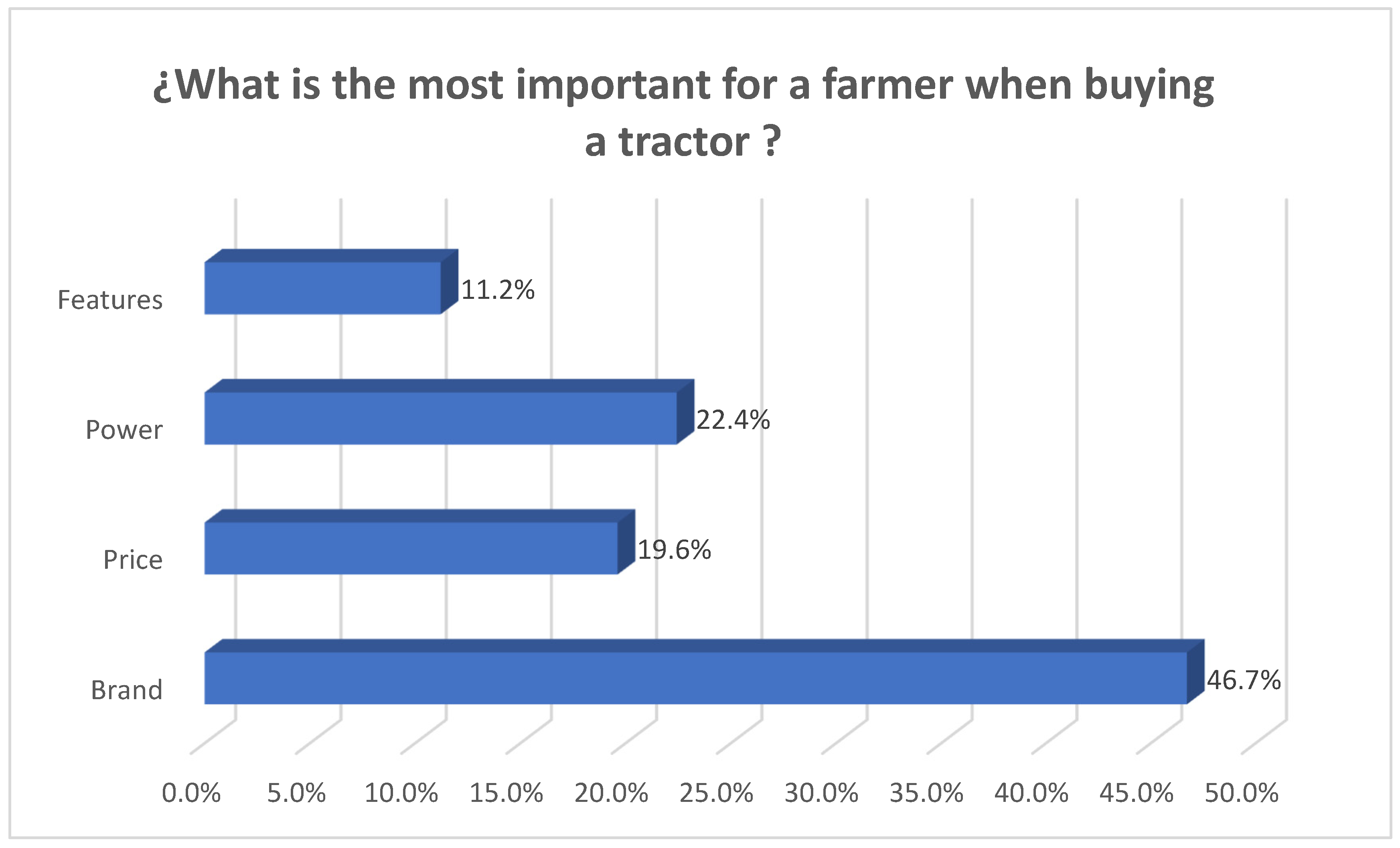
Buying a tractor represents a big investment for farmers. The most important factor for a farmer when buying a tractor is the brand, followed by power, price, and features (see Figure 1) [5].

However, in the case of purchasing a new tractor, most tractor brands do not publish prices. The farmer must go to the store to get a price estimate.

In the case of second-hand tractors, there is a very wide and varied offer. There are thousands of tractors on offer with different characteristics, operating hours, and age (year of manufacture). Thus, it is a difficult challenge for the farmer to summarize and analyze all this information.

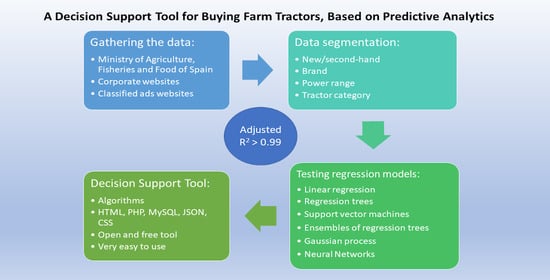
This paper attempts to solve these problems by developing a web-based DST that calculates the price of new and second-hand tractors.

Data science can help farmers when making a decision about tractor purchase. Predictive analytics can be used for estimating the price of the tractors, new and used ones. This can be used for a public or private farm consulting service.

1.1. Data Science

Data Science is an interdisciplinary field that involves scientific methods, processes, and systems to extract knowledge or a better understanding of data in its different forms, whether structured or unstructured. It includes some data analytics fields such as statistics, data mining, machine learning, and predictive analytics [6,7].

The use of data science methods and tools creates new opportunities for organizations to use data to produce new market-changing products and better public services in the data economy [6,7].

1.2. Data Economy

Data Economy can be defined as the set of initiatives, activities, and/or projects whose business model is based on the exploration and exploitation of existing database structures (traditional and from new sources) to identify opportunities for the generation of products and services.

Data are new resource considered by many as “the new oil” [8], which reflect its relevance and increasing dependence on this resource. They have also been defined as an infrastructure resource [9], as they can be used by an unlimited number of agents for an infinite number of applications to produce goods and services, considered the basic equipment and structure necessary for a country, a region, or an organization to function properly [10].

However, a piece of data by itself does not provide value. To obtain information from the data and, therefore, utility from them, it is necessary to process them.

1.3. Decision Support Tools

According to Shim et al., 2002, a DST is a computational system with the purpose of helping decision-makers by analyzing information and identifying solutions. Their goal is to link strictly computational attributes of a management information system to the judgement ability of the decision-maker [11]. Based on that, decision support tools contribute to:

(i)

The analysis of the decision environment by identifying actors, risks, constraints, consequences, etc.; and

(ii)

The structure of the decision-making procedure by setting goals and developing ways to achieve them.

A DST consists of three fundamental characteristics: a database that can store and manage internal and external information, algorithms necessary for the analysis, and an interface for communication with the user [12].

Stakeholders and farmers may encounter difficulties in making proper decisions about agricultural management in topics where there is a huge amount of information available (e.g., environmental, crop-related, and economic data) [13]. It is challenging for them to transfer these data into practical knowledge. Thus, DST can assist them in making evidence-based and precise decisions.

DST have been developed in agriculture for disease prevention [14,15], optimizing crop rotation [16], assessing the climate regulation potential of agricultural soils [17], visualizing E. coli risk on agricultural land [18], field-specific nutrient management [19], and many other applications [20]. There are studies about the development of decision support tools in other fields like medicine [21,22,23,24], supply chain management [25], cement industry [26], sewage sludge treatment [27], marine spatial planning [28], or ecosystem services quantification and valuation [29].

Rose et al., 2016, found the following eight core factors that influence the uptake and use of DST by farmers: performance expectancy, easy to use, peer recommendation, trust, cost, habit, relevance to user and farmer-adviser compatibility [20].

1.4. Tractor Cost Studies

Regarding tractor cost and prices, there are studies about tractor repair and maintenance costs [30,31,32], depreciation patterns for farm tractors [33,34,35,36,37] and farm tractor replacement modelling [38,39].

Al-Suhaibani and Wahby 2017 studied the work order for 40 tractors, investigating the relationship between tractor age and power on repair and maintenance costs, finding that repair cost ratio and maintenance cost ratio were directly related to tractor working life (age) and tractor power [30]. Asfarnia et al., 2014 studied the effect of failure rate on repair and maintenance costs of just four agricultural tractor models [31]. Lorencowicz and Uziak, 2015 studied the repair cost of tractors and agricultural machines in family farms in Poland. They found that specific circumstances of Polish agriculture, with small sizes of the farms and old tractors and agricultural machines, highly affect the repair costs [32].

Dumler et al., 2003 compared six depreciations methods to simulate the value of farm tractors in USA. The methods compared were those of the American Society of Agricultural and Biological Engineers (ASABE), Cross and Perry [36,40], North American Equipment Dealers Association (NAEDA), the Kansas Management, Analysis and Research (KMAR) plus two US income tax methods. They found that no method is consistently the most accurate, and thus farm managers must devote significant time and thought to choosing a depreciation method for their farm business [33]. This study is outdated because some of the models applied have changed.

Fenollosa and Guadalajara Olmeda, 2007 and 2010, used a dataset of new and second-hand tractor characteristics and prices with data from Spain and Italy. They studied the remaining value for financial and tax planning purposes [34,41].

Hansen and Lee, 1991 analyzed second-hand farm tractor prices to estimate farm tractor depreciation, for tax implications in Canada and USA. Their results indicated that depreciation of farm tractors would be approximated by an 8.3% annual rate [35].

Wilson, 2010, used 1223 observations of second-hand tractor prices in the UK, for estimating tractor depreciation with linear regression models. The preferred model explained 87% of the variation in total depreciation [37].

Gaworski and Jóźwiak, 2012, studied the financial advantages of purchasing new tractors in comparison with extending the life of old ones. The investigation was done in a family farm in Poland [38].

Poozesh et al., 2012 determined the economically optimum life of a single model of tractor in a certain location of Iran. Listed price of tractor, annual depreciation, and internal rate of return and repair and maintenance cost were used to determine their economic life [39].

Thus, there are studies on the cost of new and used tractors, that analyze their variables, regarding depreciation, for valuation of machinery on market value balance sheets and tax implications. None of them was applied to the development of DSTs. All of them use only parametric modeling with datasets from only one or two countries and very limited number of brands.

The main objective in the present study was to develop a DST for the decision-making procedure of buying farm tractors, for predicting tractor prices. The study includes the use of parametric and non-parametric models.

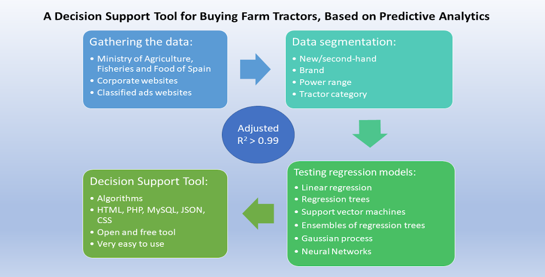
2. Materials and Methods

In this study there is a combination of open data from the public sector (Ministry of Agriculture, Fisheries and Food of Spain–MAPA), data from corporative websites of tractor brands, and data from classified ads websites (Agriaffaires, Tractorhouse, Mascus, Truck1.eu and E-farm.com).

The dataset includes observations from Spain, Portugal, Germany, France, Italy, Belgium, Poland, and United Kingdom.

Regarding the new tractors, we searched data about 27 different brands, including the most important brands in the European market (see

Table 2. Top brands of new tractor sales in Europe in the year 2020 [3].

Brand	Tractors Sold	Market Share
John Deere	28,655	18.26%
New Holland	20,979	13.37%
Fendt-Challenger	17,544	11.18%
Case Ih/Steyr	12,206	7.78%
Massey Ferguson	10,794	6.88%
Claas	9690	6.18%
Deutz-Fahr	9139	5.82%
Kubota	9105	5.80%
Valtra	7615	4.85%
Same	3197	2.04%
Landini	2358	1.50%
Steyr	1626	1.04%
Lamborghini	1374	0.88%
McCormick	903	0.58%
Hürliman	214	0.14%
Valpadana	148	0.09%
Other	21,356	13.61%

) [3]. They were the following: John Deere, Case IH, New Holland, Steyr, Massey Ferguson, Same, Lamborghini, Deutz-fahr, Valtra, Landini, Claas, Kubota, Antonio Carraro, Pasquali, Mc Cormick, Valpadana, Ferrari, Goldoni, Arbos, Kioti, Iseki, BCS, Agria, Zetor, Belarus, Yanmar, Ursus.

We searched information on 27 brands, but we got data from 15 of these brands. This is because for some of the brands there was no open information on the price of new tractors. We got observations about 227 models of new tractors. For each model, the data includes brand, power, and price. The data about brand, model, category, and power were cross-checked with the official ministry database.

In the case of second-hand tractors, data were collected for all the brands listed in tractor advertisements on the consulted websites. To avoid errors in the information collected on these sites, the data about brand, model, category, and power were also cross-checked with the official database from the Ministry.

We obtained data on 1003 observations of second-hand/used tractors. Each observation includes brand, model, category, power, operating hours, and/or age (year of manufacture) of each tractor. Sometimes, the number of operating hours or the age was missed. The data about brand, model, category, and power were also cross-checked, with the official ministry database.

2.1. Data Recording and Storage

The open data from MAPA was downloaded, the data from corporate websites were taken manually, and the data from classified ads websites were scrapped using a script developed with Phyton.

All of these data were combined and stored in a MySQL 5.7 ad hoc database. For making queries to the data database, PHP 7.4.21 was used. The information was shown using an HTML 5, CSS 3 interface. Thus, data can be visualized with any Web browser.

2.2. Data Analysis

Microsoft Excel 365 and Matlab R2021b were used to analyze the data and produce the figures. Several types and subtypes of parametric and non-parametric regression models were trained and validated in order to find the best one for the dataset. Regression is a method for estimating the relationship between a response variable (dependent variable, output, target) and one or more predictor variables (independent variables, explanatory variables input) [42,43]. In this study, the models tested included linear regression, regression trees, support vector machines (SVM), ensembles of regression trees, Gaussian process regression models (GPR), and regression neural networks (see

Table 3. Regression models tested.

Type of Model	Subtype
Linear regression	Linear
	Interactions linear
	Robust linear
	Stepwise linear
Regression trees	Fine tree
	Medium tree
	Coarse tree
Support vector machines	Linear SVM
	Quadratic SVM
	Cubic SVM
	Fine Gaussian SVM
	Medium Gaussian SVM
	Coarse Gaussian SVM
Ensembles of regression trees	Boosted Trees
	Bagged Trees
Gaussian process	Squared Exponential
	Matern 5/2 GPR
	Exponential GPR
	Rational Quadratic GPR
Neural Networks	Narrow Neural Network
	Medium Neural Network
	Wide Neural Network
	Bilayered Neural Network
	Trilayered Neural Network

).

In the case of new tractors, the dependent variable was price (variable Y), and the independent variable was power (variable X). For second-hand tractors, the dependent variable was also price, and the predictor variables were power, hours of use, and year of manufacture (age).

In general, the best model is the model with the highest adjusted R², and the lowest RMSE (root mean squared error). However, the model must be consistent with the knowledge of the data and its environment should be also taken into account.

The adjusted R² is an evaluation metric better than R². R² is a statistical measure that represents the proportion of variation in the response variable explained by the regression model. The adjusted R² adds precision and reliability by considering the impact of additional predictor variables that tend to skew the results of R² measurements. The adjusted R² formula is

$${\mathrm{Adjusted}\mathrm{R}}^2=1-\left(1-{\mathrm{R}}^2\right)\frac{\mathrm{n}-1}{\mathrm{n}-\mathrm{p}-1}$$

(1)

where n is the number of observations and p is the number of independent variables [42,43].

Polynomial and exponential regressions manage to add curvature to the model by introducing new predictors obtained by raising all or some of the original predictors to different powers. In all the analyses, the order of the polynomials was kept as low as possible, in order to avoid abuse of the regression analysis.

2.3. Robust Modeling

In order to minimize the influence of outliers in linear regression, several weight (W) functions were tested for fitting the data, including Andrews, Bisquare [44], Cauchy, Fair, Huber [44], Talwar, Welsch (see

Table 4. Robust modeling functions tested.

Weight Function	Description	Default Tuning Constant
Andrews	$\mathrm{If}\left|\mathrm{r}\right|<\mathsf{\pi }\mathrm{W}=\frac{\sin \left(\mathrm{r}\right)}{\mathrm{r}}$ $\mathrm{If}\left|\mathrm{r}\right|\ge \mathsf{\pi }$ W = 0	1.339
Bisquare	$\mathrm{If}\left|\mathrm{r}\right|<1\mathrm{W}={\left(1-{\mathrm{r}}^2\right)}^2$ $\mathrm{If}\left|\mathrm{r}\right|\ge 1$ W = 0	4.685
Cauchy	$\mathrm{W}=\frac{1}{\left(1+{\mathrm{r}}^2\right)}$	2.385
Fair	$\mathrm{W}=\frac{1}{\left(1+\left|\mathrm{r}\right|\right)}$	1.400
Huber	$\mathrm{If}\left|\mathrm{r}\right|\ge 1\mathrm{W}=\frac{1}{\left|\mathrm{r}\right|}$ $\mathrm{If}\left|\mathrm{r}\right|<1\mathrm{W}=1$	1.345
Talwar	If |r|<1 W = 1 If |r|>1 W = 0	2.795
Welsch	W = exp(−(r2))	2.985

) and also least absolute residuals (LAR) [43,45].

The value of r in the weight functions is

$$\mathrm{r}=\frac{\mathrm{resid}}{\mathrm{tune}·\mathrm{s}·\sqrt{1-\mathrm{h}}}$$

(2)

where

resid is the vector of residuals from the previous iteration.

tune is the tuning constant.

h is the vector of leverage values from a least-squares fit.

s is an estimate of the standard deviation of the error term.

The LAR method finds a curve that minimizes the absolute difference of the residuals, rather than the squared differences. Therefore, extreme values have less influence on the fit.

$$MAE=\min {\displaystyle \sum }_{i=1}^n\left|y_i-{\widehat{y}}_{i|}\right|$$

(3)

These methods were tested, and the ones that got the highest adjusted R² and lowest RMSE were chosen.

2.4. Data Segmentation

Several segmentations of the data were made: new/second-hand, by brand, by power range, and by tractor category.

The power ranges into which the analysis was divided were: 0–50 kW, 51–150 kW, 151–250 kW, 251 kW or more.

Regarding the segmentation by categories, the official classification of MAPA was used. In this classification, there are the 15 categories of tractors (MAPA, 2021b):

• Microtractors (for Gardening)
• Crawler Tractors
• Tractors with Platform
• Wheel Tractors
• Wheel Tractors with More Than Two Axles
• 4WD Tractor
• 4WD Narrow and Articulated Tractor
• 4WD Normal Width and Articulated Tractor
• 4WD Narrow Tractor
• 4WD Normal Width Tractor
• 2WD Tractor
• 2WD Narrow Tractor
• 2WD Normal Width Tractor
• Tool Carrier Tractor
• Semi Crawler Tractor (Semi Tracked)

In all of these data segmentation, only datasets with 5 or more data points were taken into account.

2.5. Decision Support Tool Development

The web tool was developed, implemented and validated on-line, in a real environment. The programming languages used were HTML, PHP, MySQL, JSON, and CSS.

3. Results

3.1. New Tractors

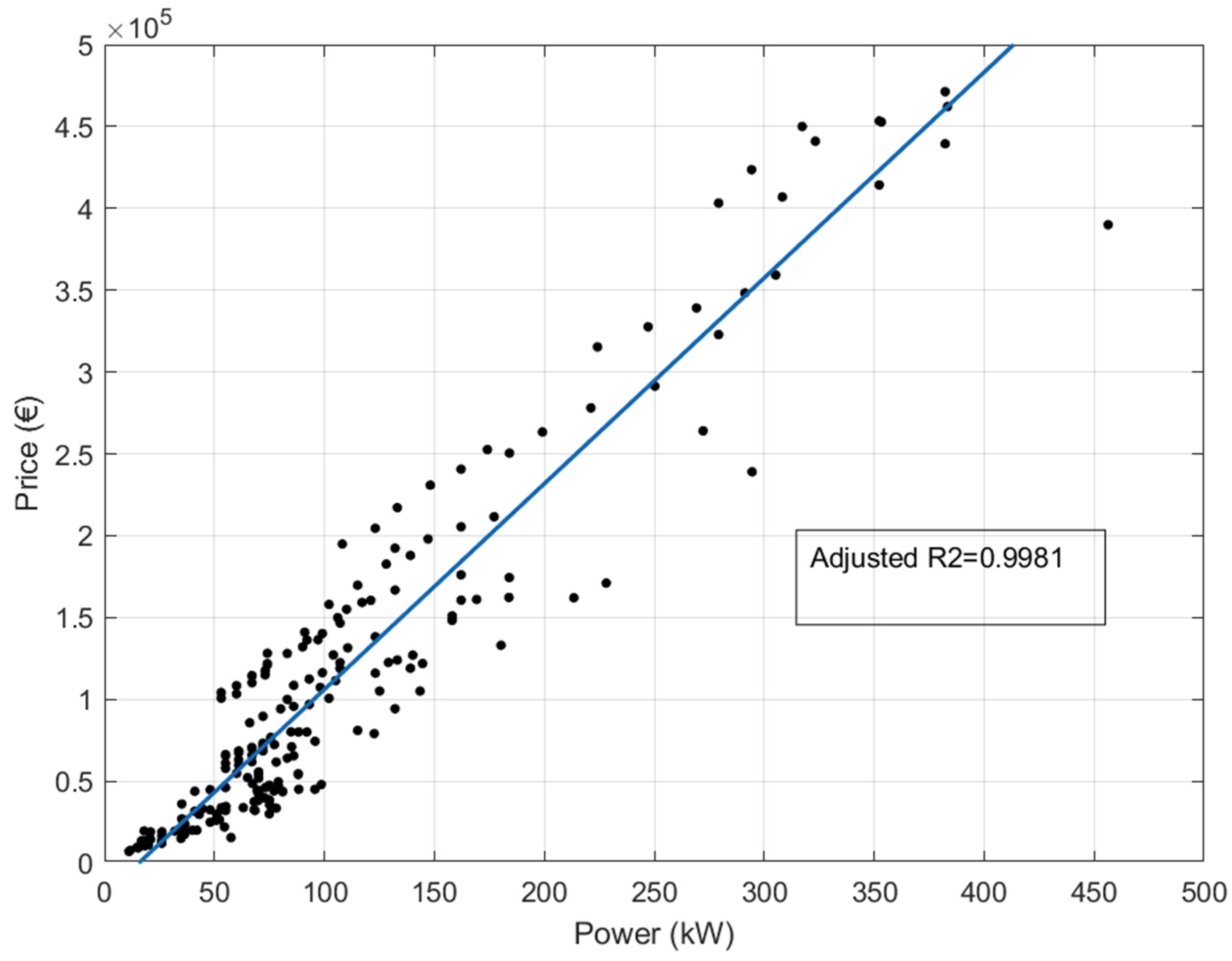
With the new tractor’s dataset, 227 observations from 15 brands, several regression models were tested Price vs. Power.

Table 5. Results from regression models testing with the whole new tractors dataset.

Type of Model	Subtype	Adjusted R2
Linear regression	Linear	0.8872
	Interactions linear	0.8996
	Robust linear	0.9981
	Stepwise linear	0.8946
Regression trees	Fine tree	0.8895
	Medium tree	0.8493
	Coarse tree	0.7087
Support vector machines	Linear SVM	0.8996
	Quadratic SVM	0.8895
	Cubic SVM	0.8841
	Fine Gaussian SVM	0.8795
	Medium Gaussian SVM	0.9096
	Coarse Gaussian SVM	0.8996
Ensembles of regression trees	Boosted Trees	0.8895
	Bagged Trees	0.8906
Gaussian process	Squared Exponential	0.9026
	Matern 5/2 GPR	0.9076
	Exponential GPR	0.8996
	Rational Quadratic GPR	0.9086
Neural Networks	Narrow Neural Network	0.9072
	Medium Neural Network	0.9091
	Wide Neural Network	0.8966
	Bilayered Neural Network	0.9082
	Trilayered Neural Network	0.9096

shows the results.

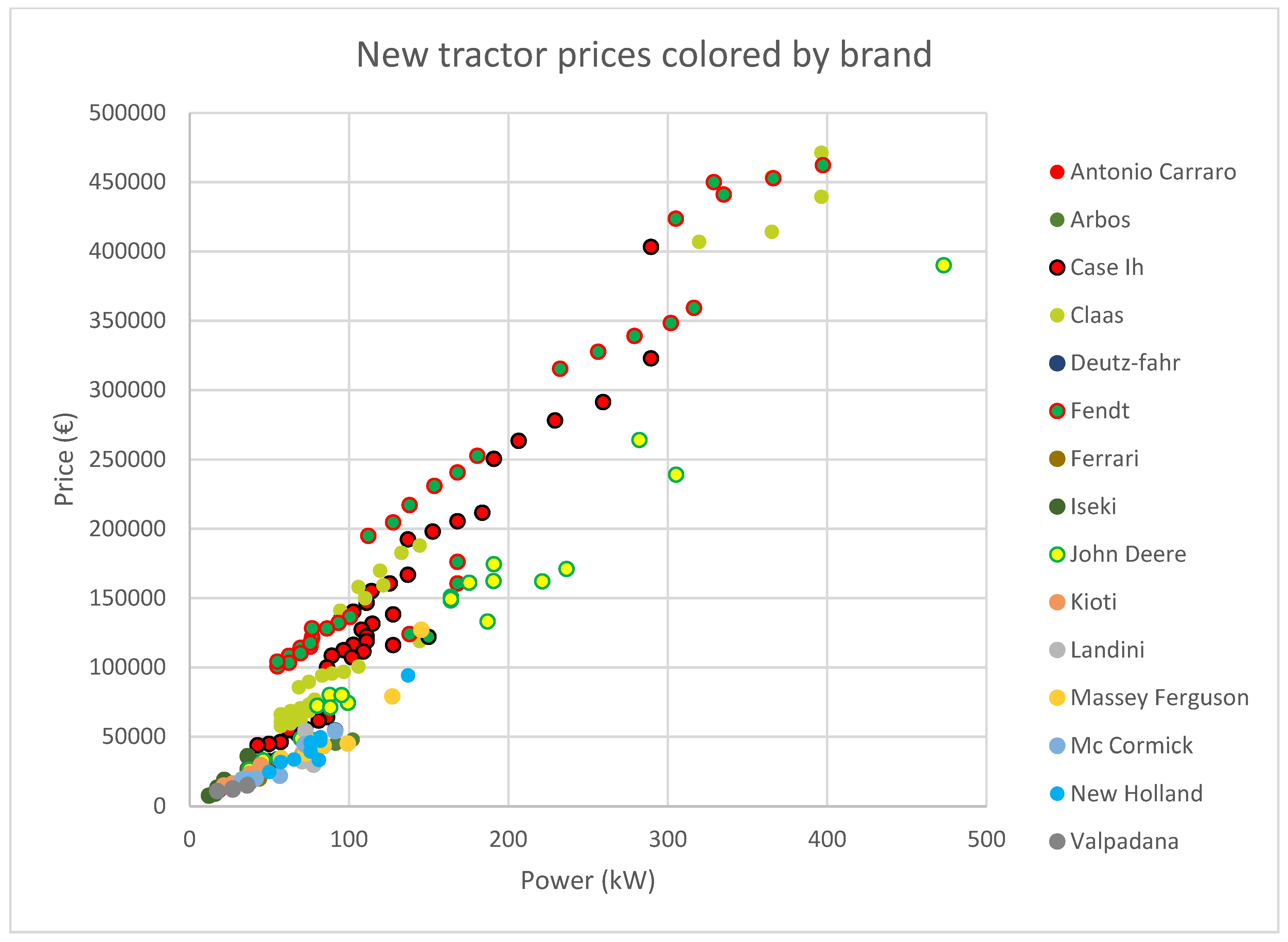
Best results were found with robust linear regression (see Table 5 and Figure 2). The best fit was in a polynomial model of degree 1 using LAR robust adjustment. With this model, the adjusted R² was 0.9981 (see Figure 2). Thus, it is possible to predict the price of a new tractor, knowing its power, regardless of its brand (see Figure 3).

For the new tractor dataset, more sophisticated regression models like regression trees, SVM, ensembles of regression trees, Gaussian process, and Neural Networks, do not provide better results than robust linear regression (see Table 5).

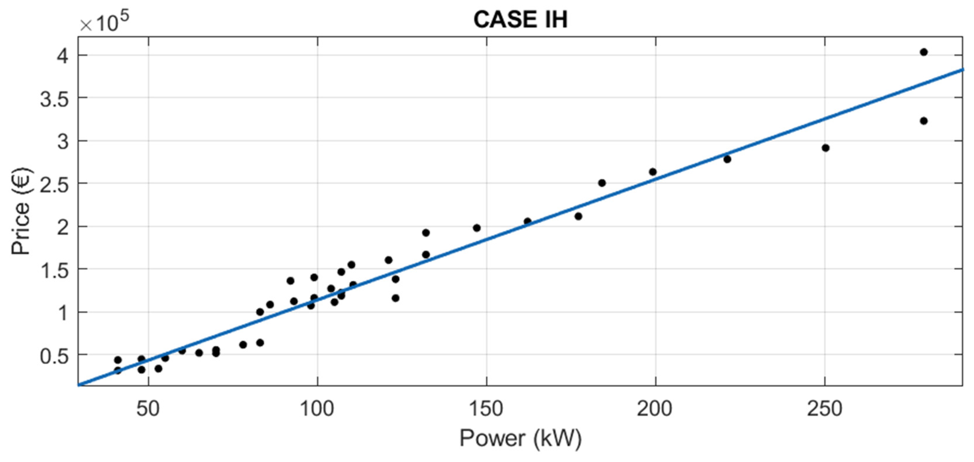
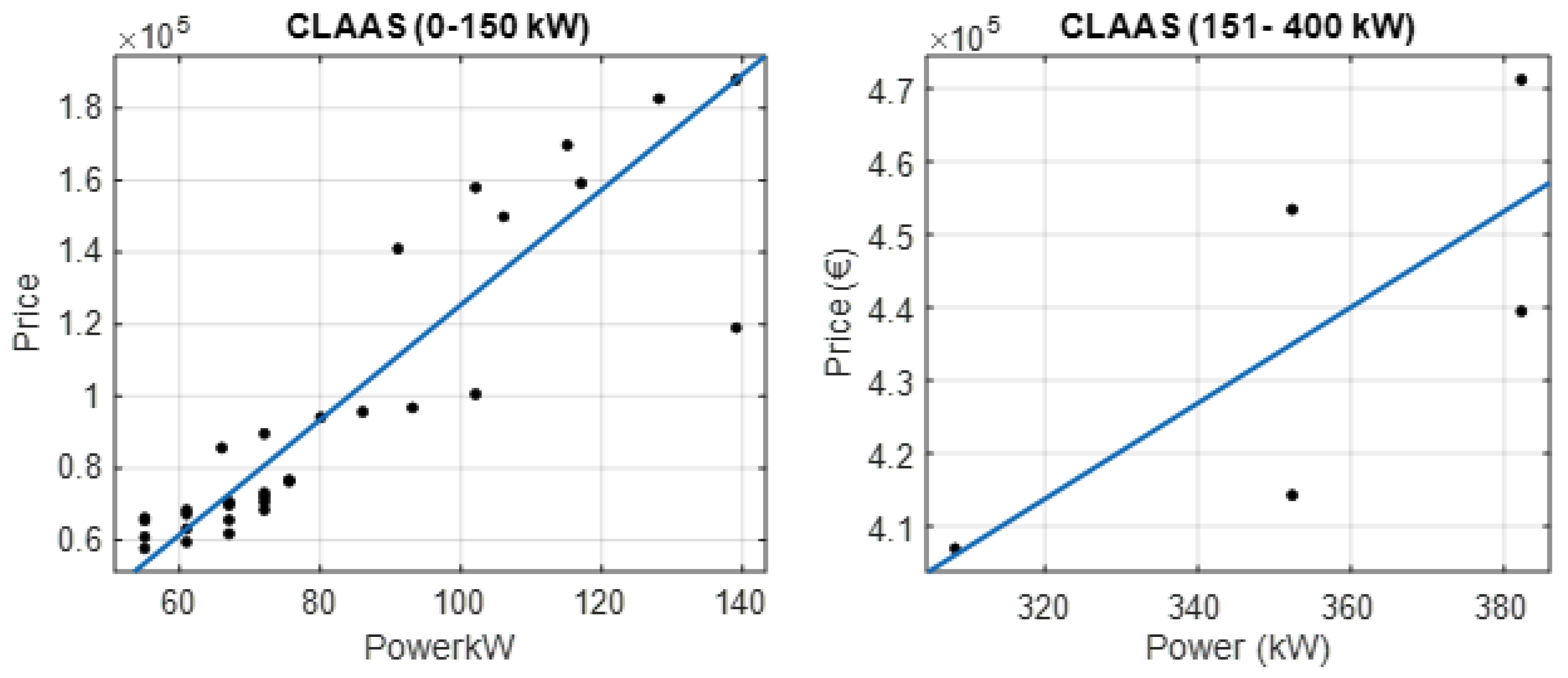
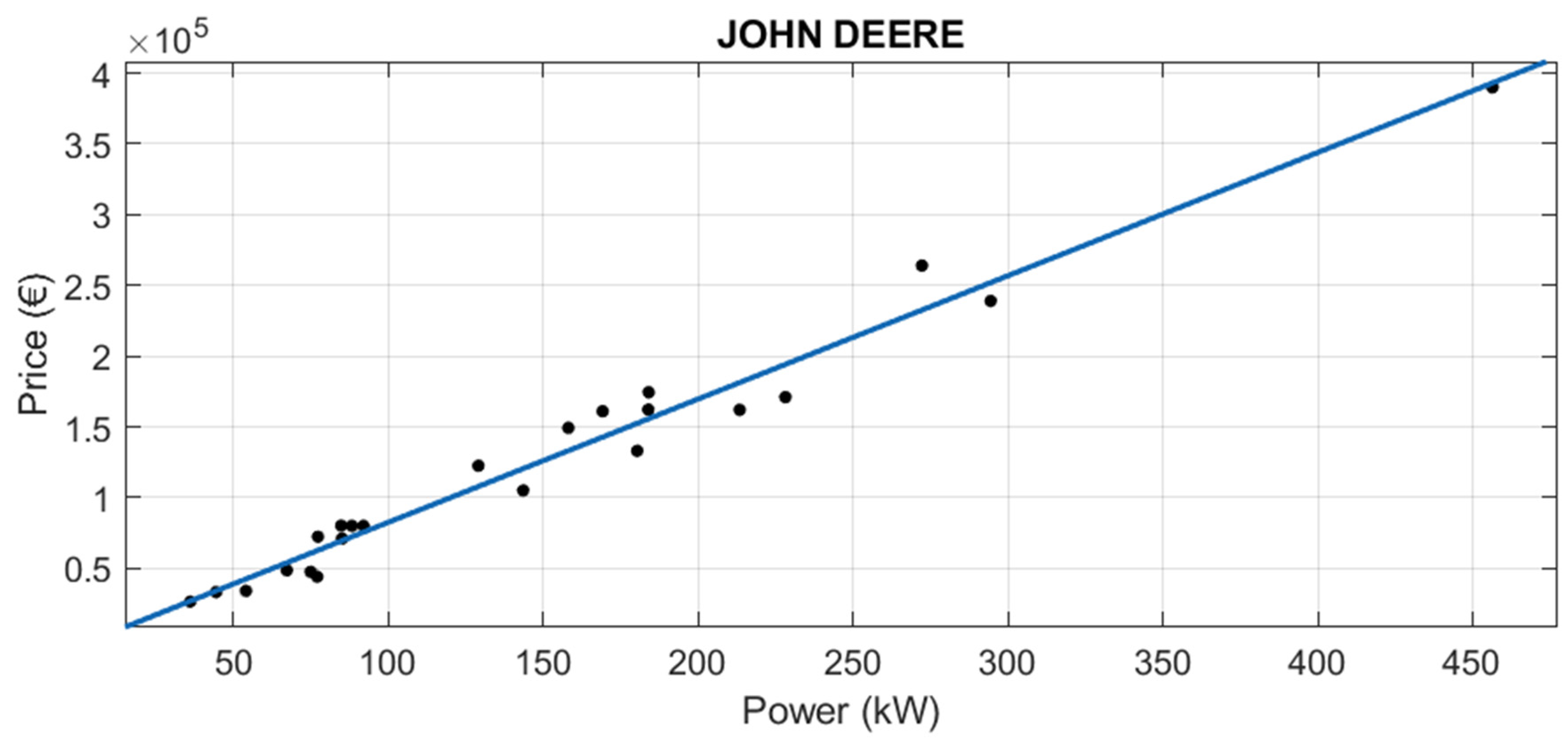
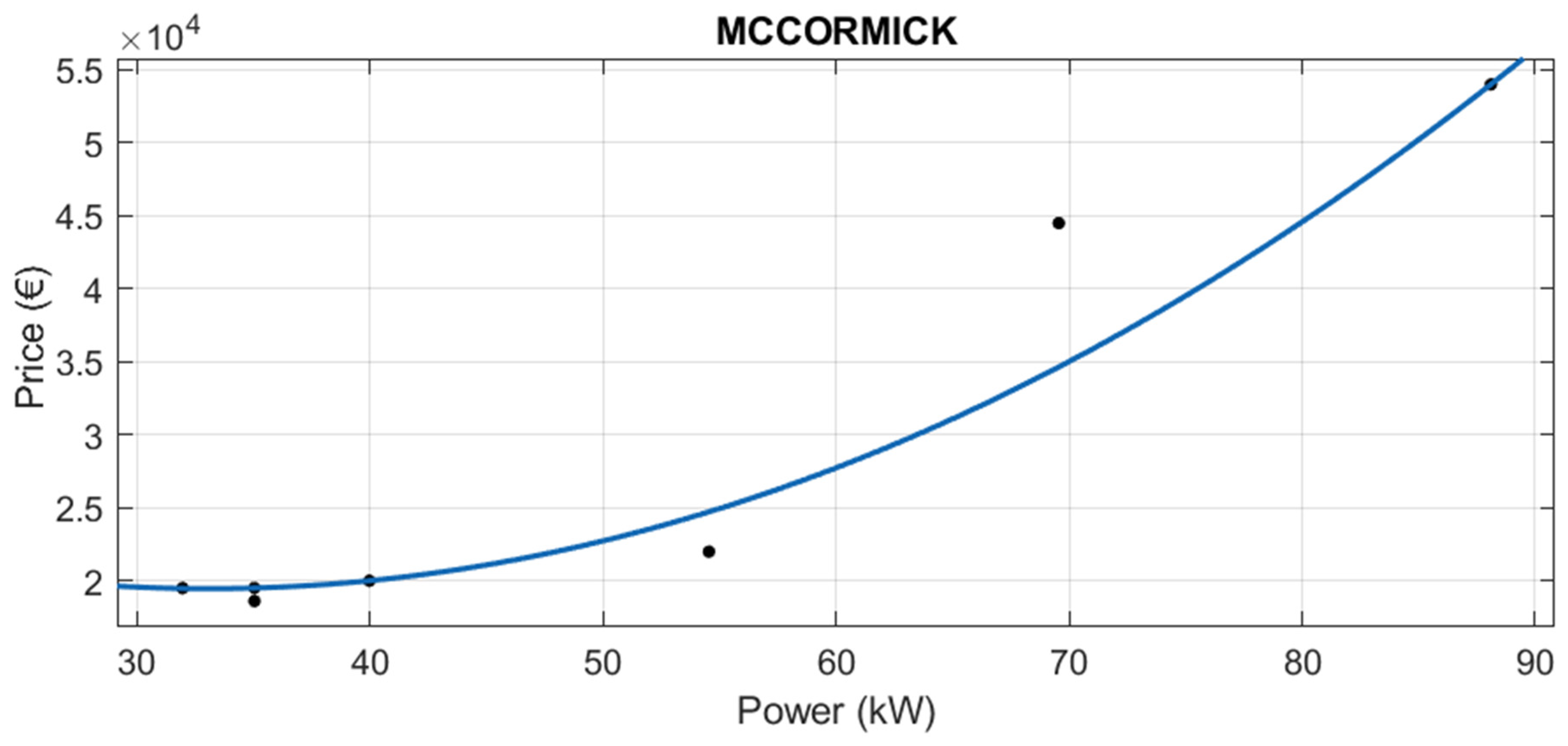
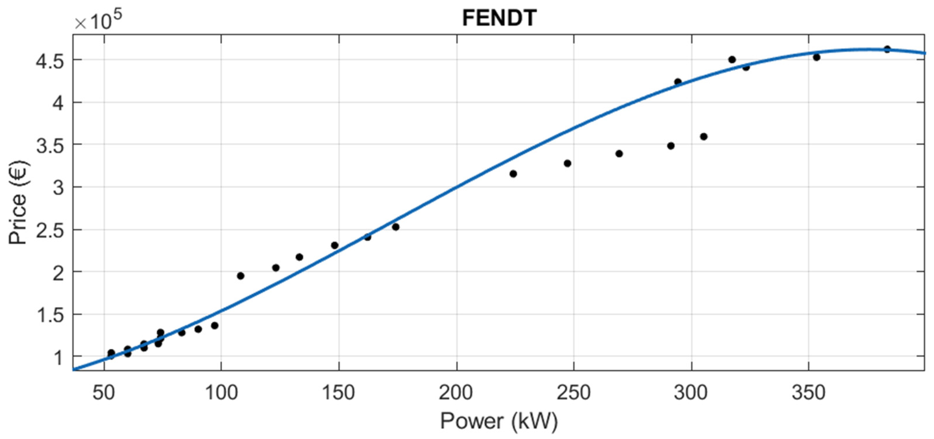
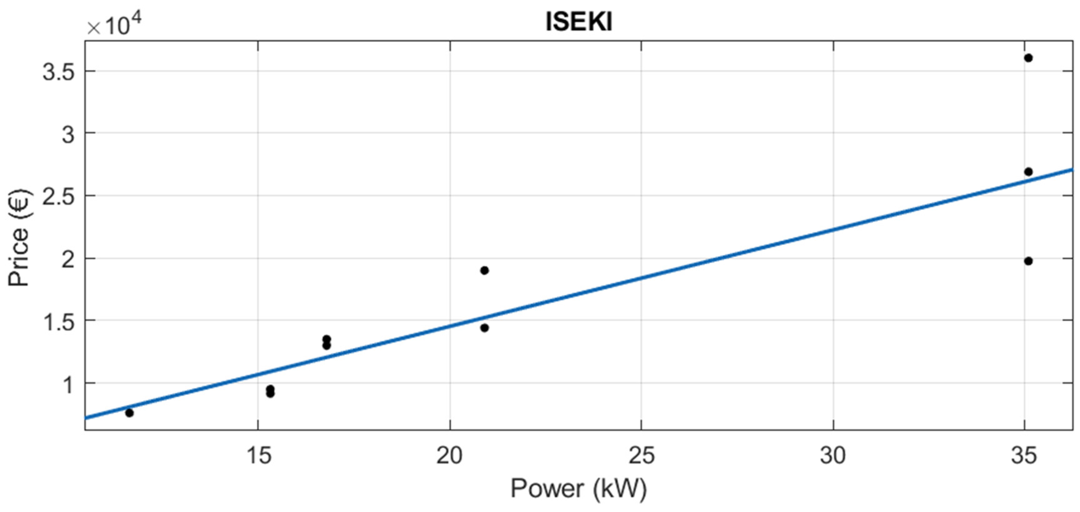
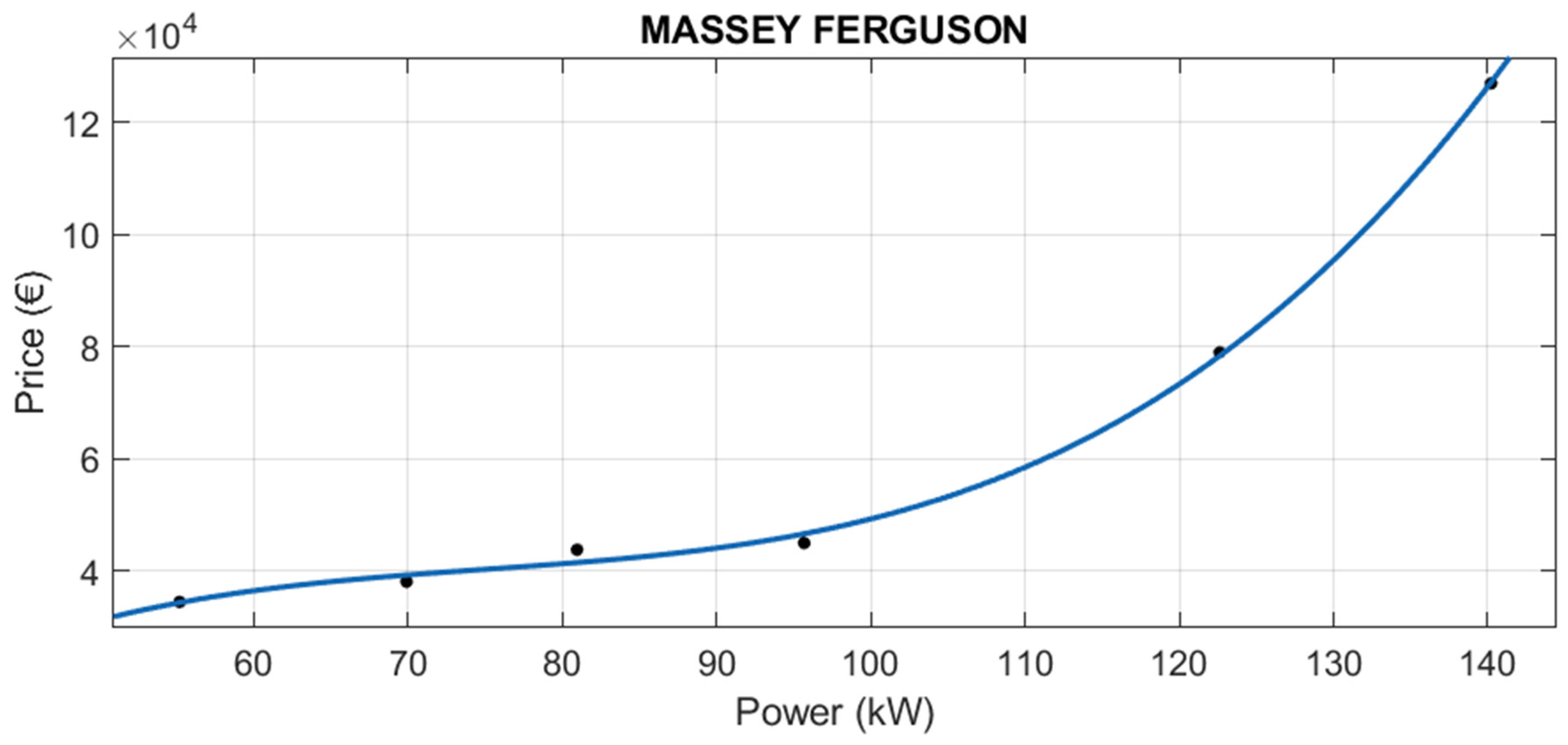
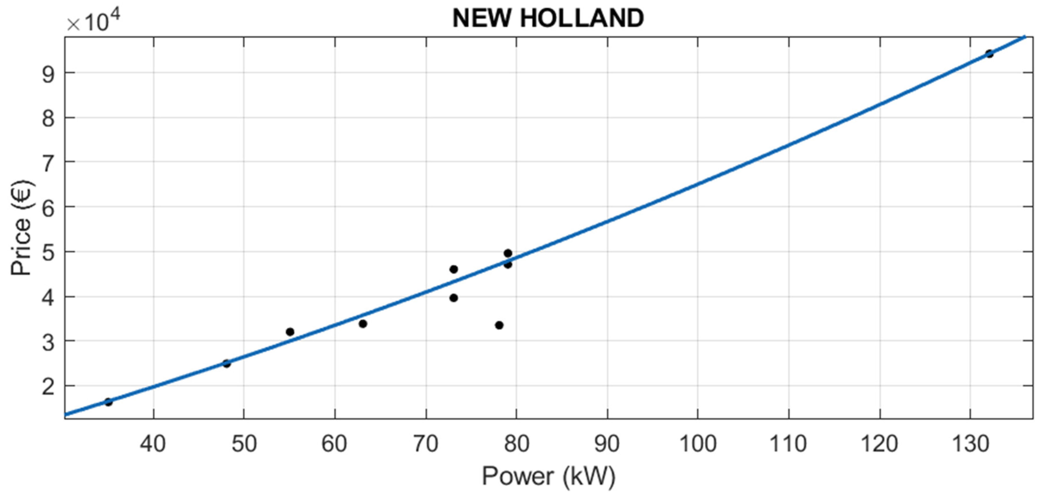
3.1.1. Segmentation by Brand

Of the 24 brands for which data were available, 8 of them had more than 5 data and regressions were performed (see Figure 4, Figure 5, Figure 6, Figure 7, Figure 8, Figure 9, Figure 10 and Figure 11 and

Table 6. Summary of best results with new tractors data by brands.

Brand	Model Type	Adjusted R2
Case IH	Polynomial degree 1	0.9581
Claas (0–150 kW)	Polynomial degree 2	0.9870
Claas (151–400 kW)	Polynomial degree 1	0.4068
Fendt	Polynomial degree 3	0.9893
Iseki	Polynomial degree 1	0.8524
John Deere	Polynomial degree 1	0.9702
Massey Ferguson	Polynomial degree 3	0.9962
McCormick	Polynomial degree 2	0.9486
New Holland	Polynomial degree 2	0.9639

).

The adjusted value of R² reflects the precision of the calculation of the predicted variable (price). Therefore, the better the equation, the closer its value is to 1. Almost all the brands have adjusted R² over 0.94, with the exception of Iseki, whose R² is 0.8524 and the additional segmentation done in Claas.

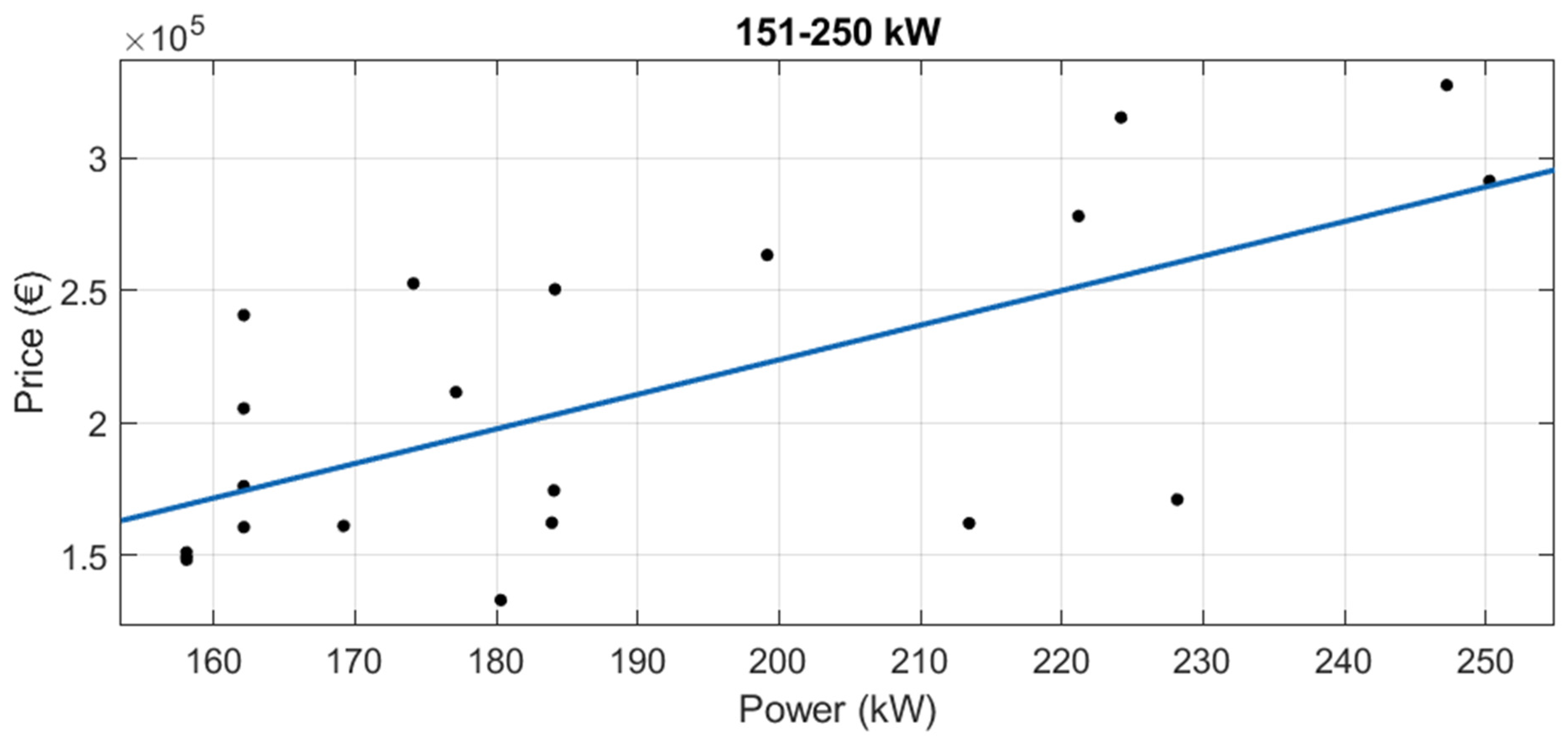
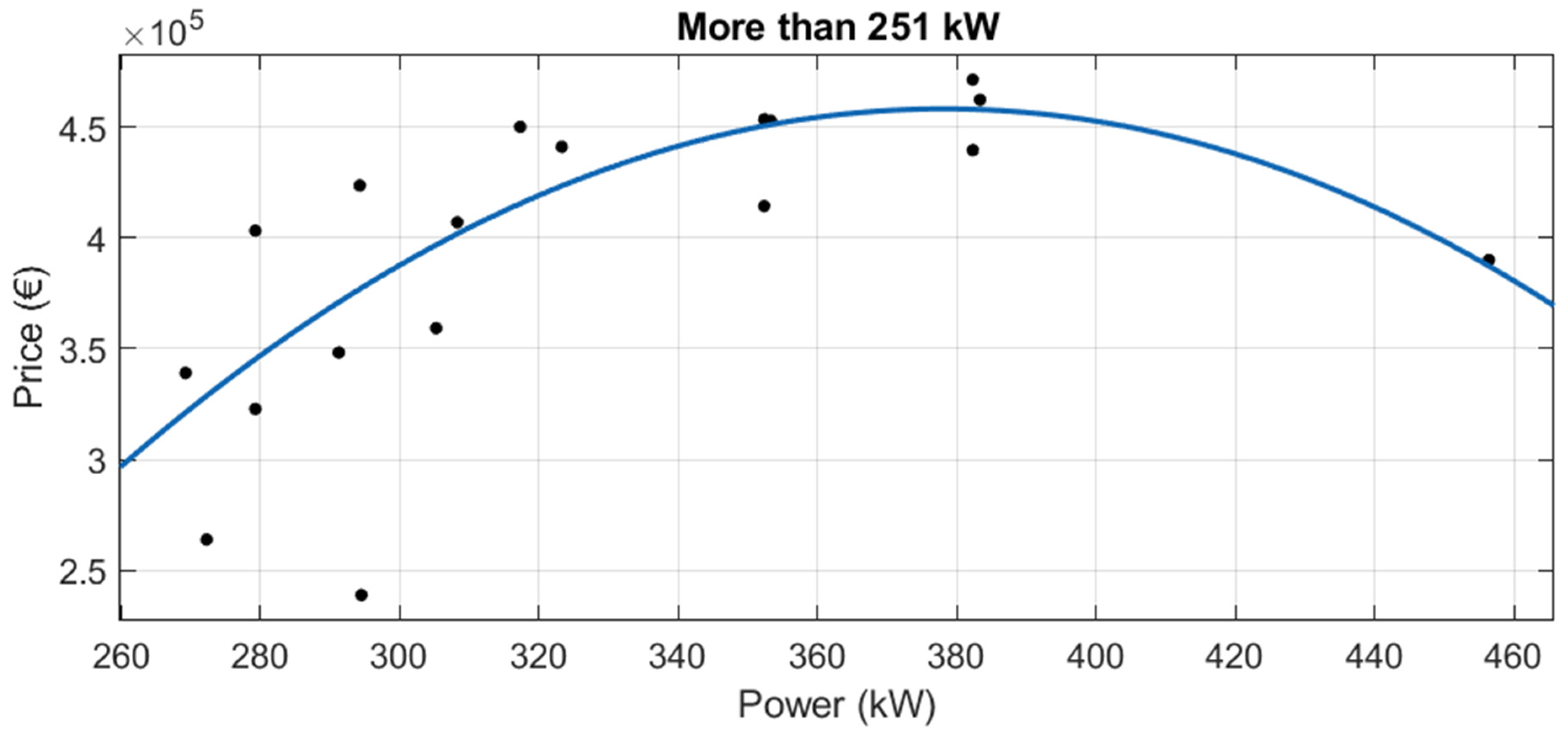
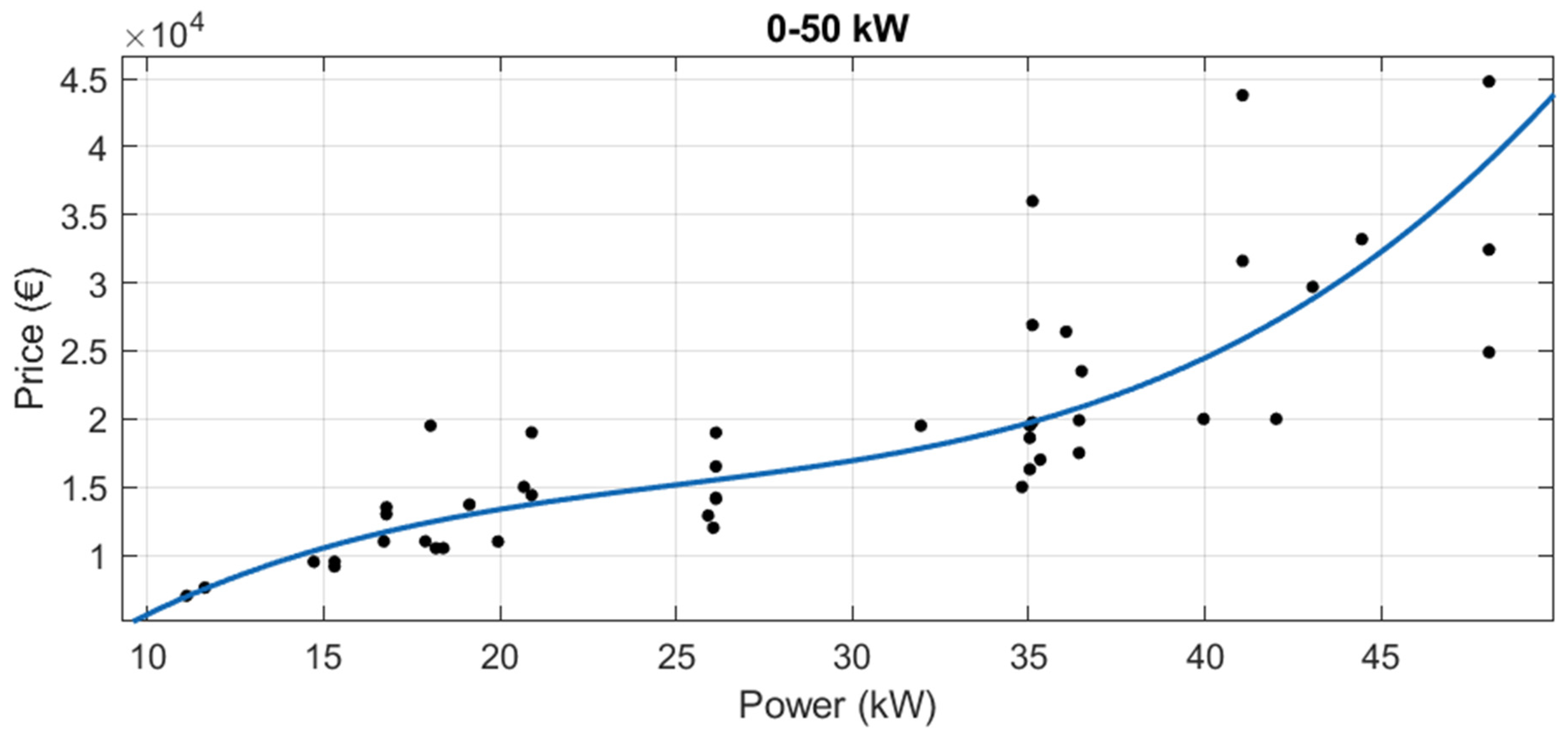
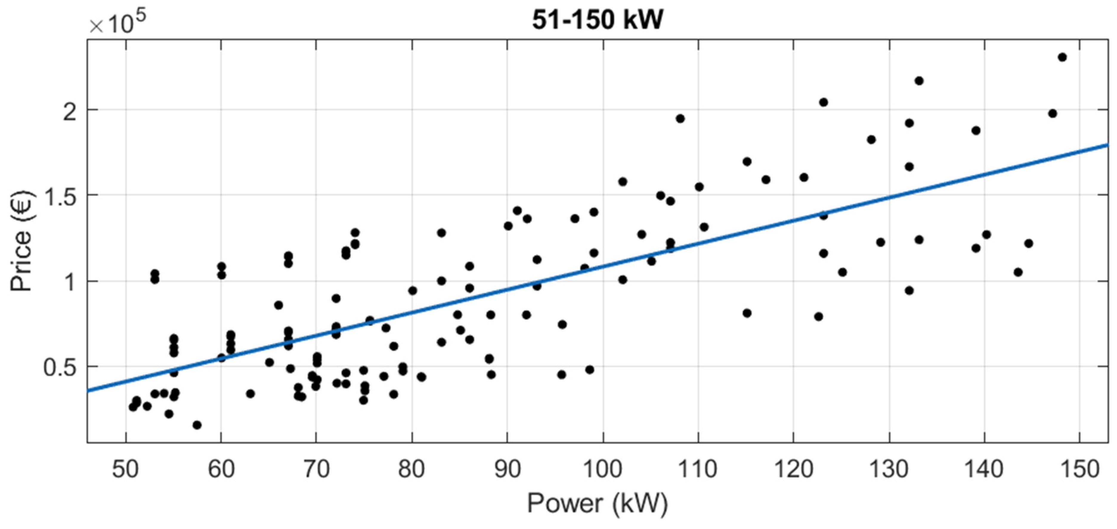
3.1.2. Segmentation by Power

In new tractors, when segmenting by power range, the results were worse than those with the whole dataset and the segmentation by brand (see Figure 12, Figure 13, Figure 14 and Figure 15 and

Table 7. Summary of results of segmentation by power for new tractors.

Power (kW)	Model Type	Adjusted R2
0–50	Polynomial degree 3	0.7814
51–150	Polynomial degree 2	0.5334
151–250	Polynomial degree 1	0.3938
More than 251	Polynomial degree 2	0.6076

). With this segmentation by power, all adjusted R² were under 0.8.

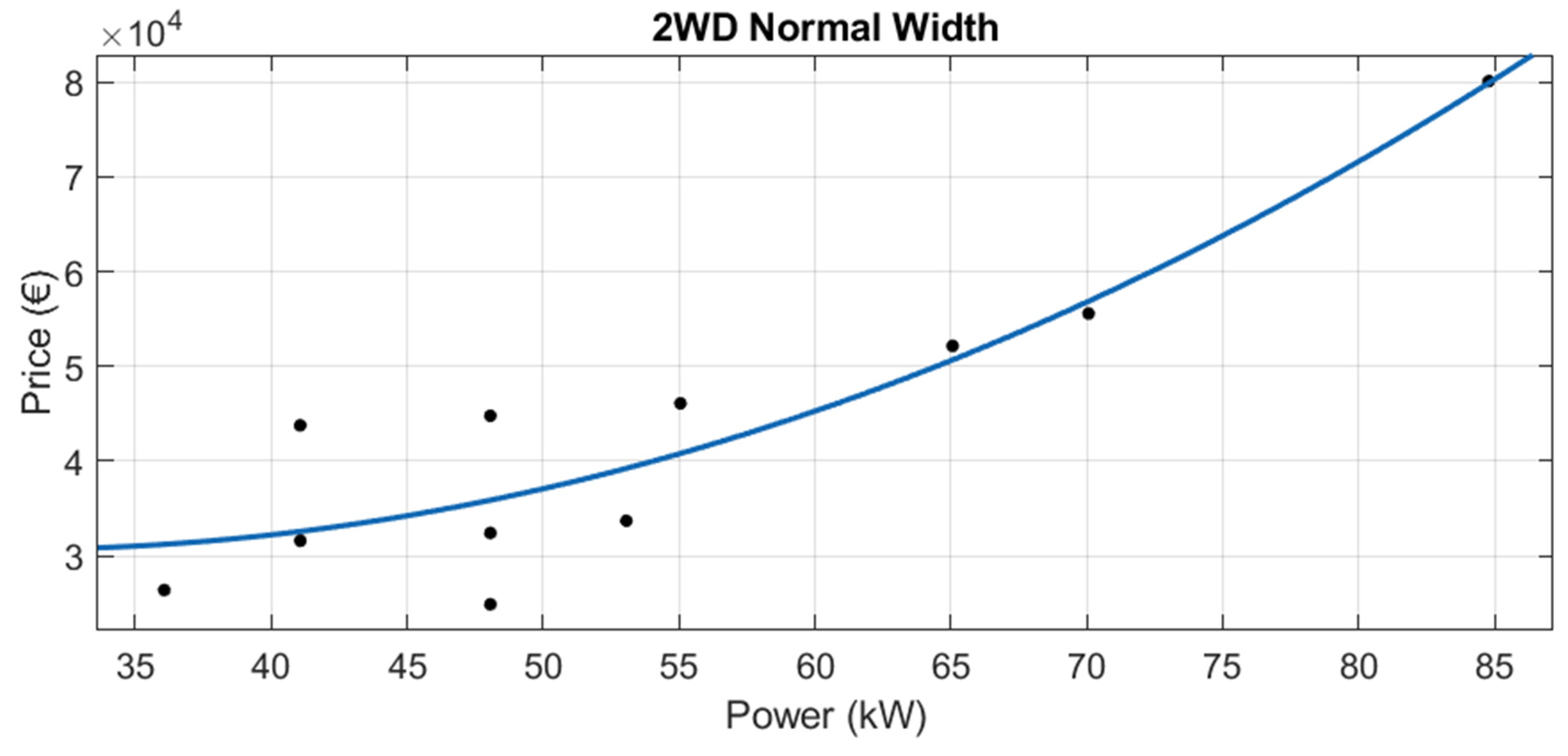
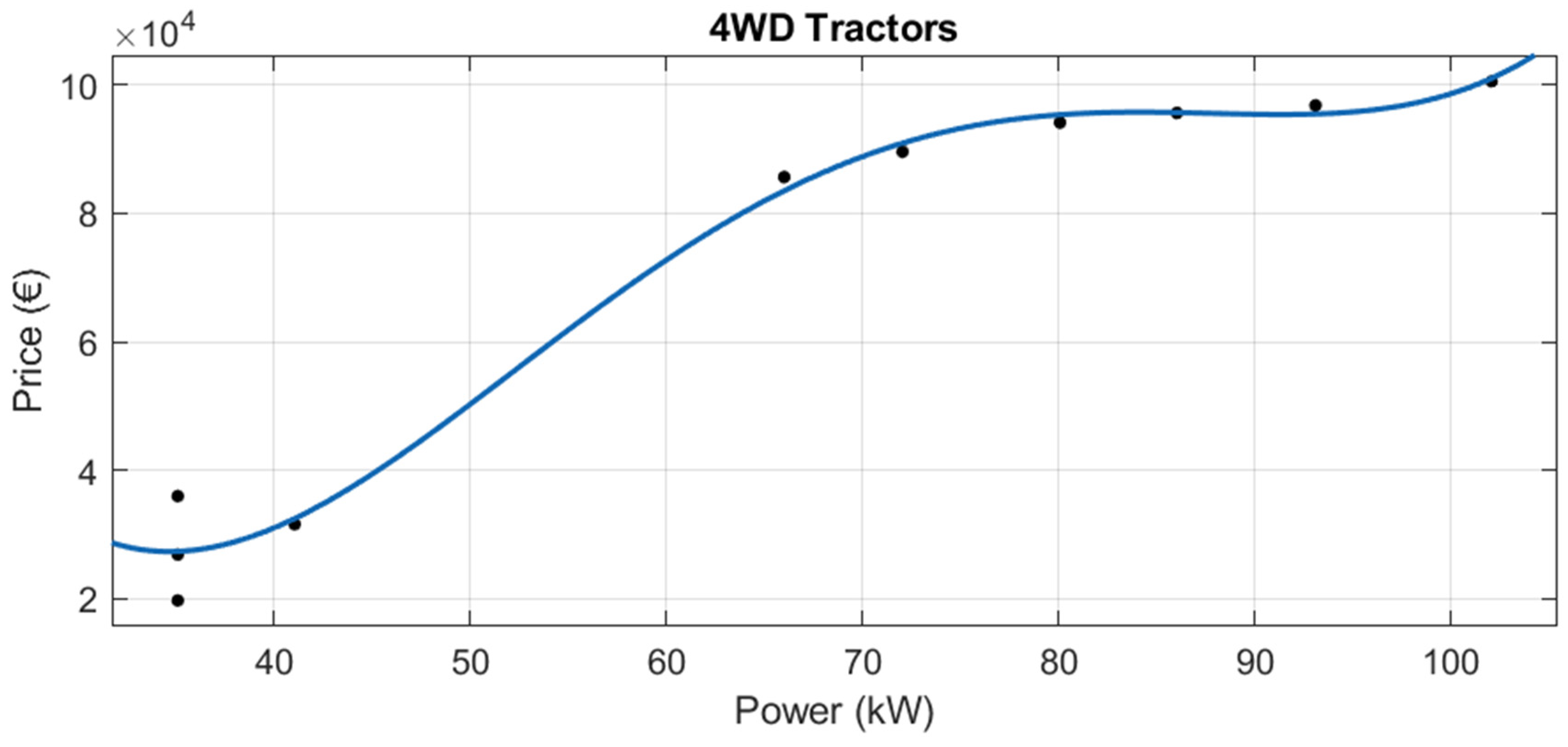
3.1.3. Segmentation by Category

Although there are 15 tractor categories in the official list, some of them are in disuse, and in others there are few models. Therefore, new tractor data were obtained for the following eight categories:

• 4WD Normal Width Tractors
• 4WD Narrow Tractors
• Crawler Tractors
• 2WD Normal Width Tractors
• 2WD Narrow Tractors
• 4WD Tractors
• Semi Crawler Tractors (Semi Tracked)
• 4WD Narrow and Articulated Tractors

Of these 8, for “Crawler Tractors”, “Semi Crawler Tractor (Semi Tracked)” and “4WD Narrow and Articulated Tractor”, very little new tractor data were available, so regression was not performed in these three cases.

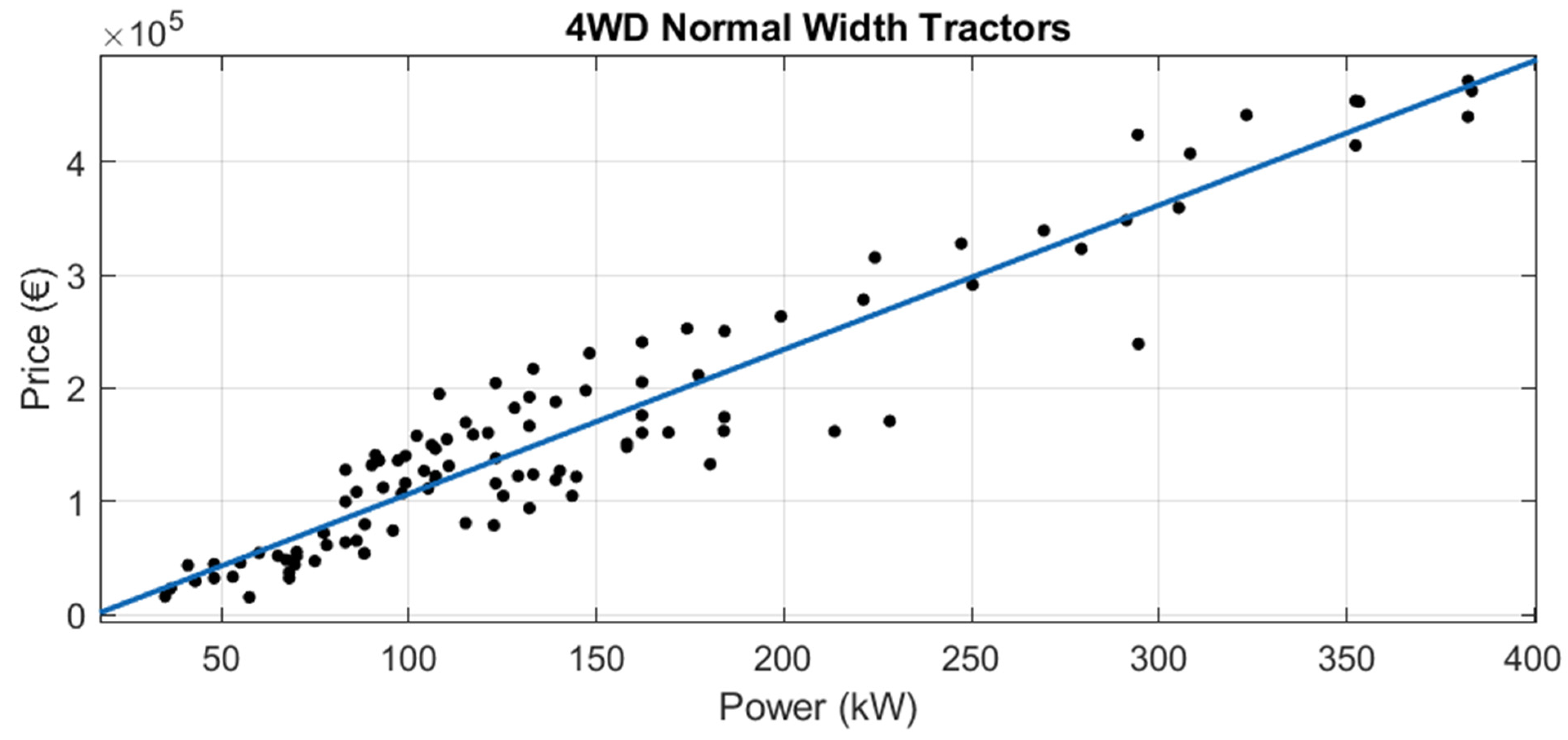
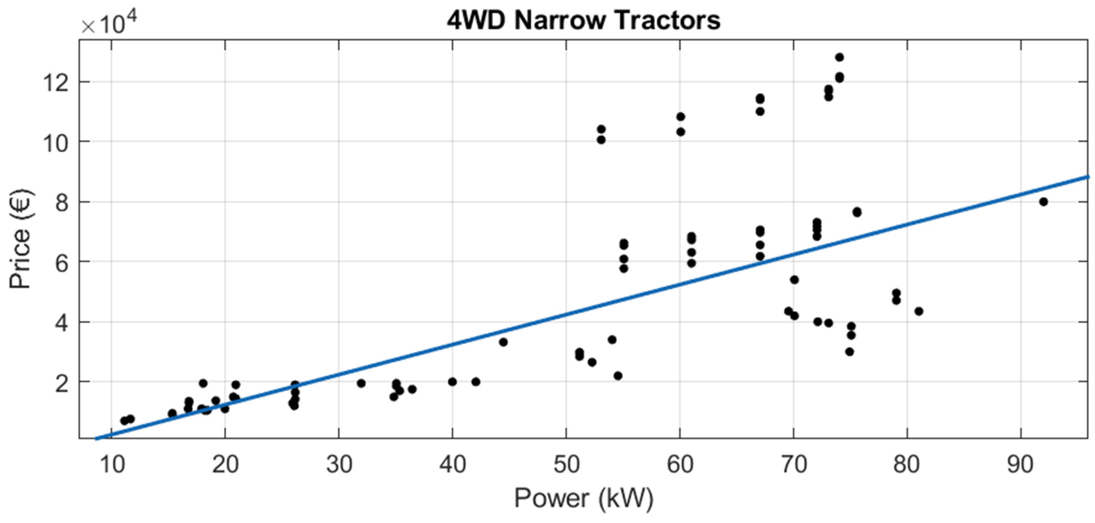
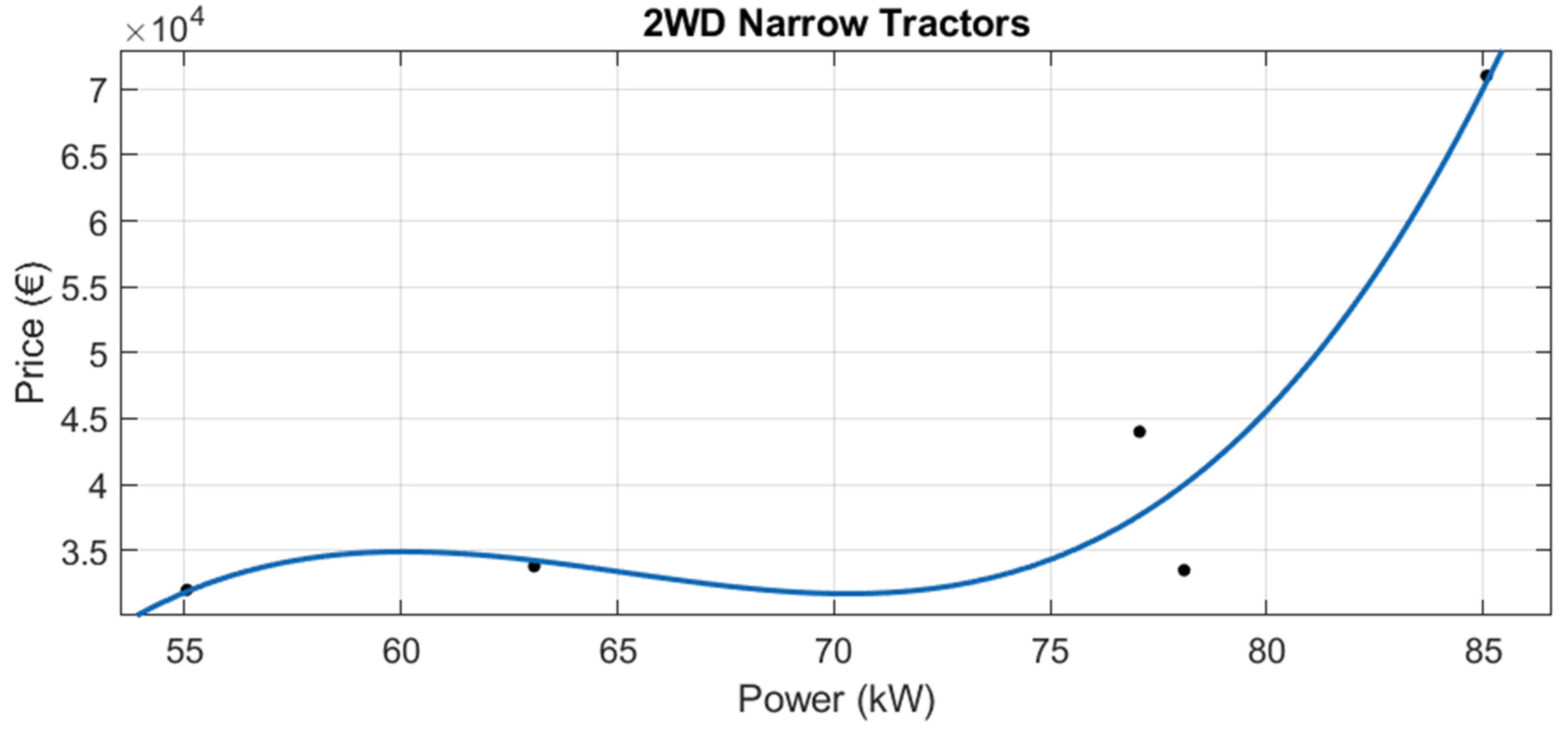
For the other six official categories, robust linear regressions were performed (see Figure 16, Figure 17, Figure 18, Figure 19 and Figure 20 and

Table 8. Summary of results of segmentation by category for new tractors.

Category	Model Type	Adjusted R2
4WD Normal Width Tractors	Polynomial degree 1	0.8950
4WD Narrow Tractors	Polynomial degree 1	0.6287
2WD Normal Width Tractors	Polynomial degree 2	0.7933
2WD Narrow Tractors	Polynomial degree 3	0.6942
4WD Tractors	Polynomial degree 4	0.9760

). Adjusted R² ranges from 0.6287 to 0.9760. The lowest adjusted R² was for “4WD Narrow Tractors” (adjusted R² = 0.6287). The highest adjusted R² was for the category “4WD Tractors” (adjusted R² = 0.9760).

3.2. Second-Hand Tractors

In this section, there is a selection of the most relevant results from the analyses performed with the second-hand tractor dataset. This dataset had 1003 observations from 56 different brands. With this dataset, several regression models were tested using three predictor variables: power, year of manufacture, and operating hours.

Table 9. Results from regression models testing, with the whole second-hand tractor dataset.

Type of Model	Subtype	Adjusted R2
Linear regression	Linear	0.8451
	Interactions linear	0.8295
	Robust linear	0.8870
	Stepwise linear	0.8295
Regression trees	Fine tree	0.7793
	Medium tree	0.7693
	Coarse tree	0.7392
Support vector machines	Linear SVM	0.7290
	Quadratic SVM	0.8395
	Cubic SVM	0.7391
	Fine Gaussian SVM	0.7894
	Medium Gaussian SVM	0.8492
	Coarse Gaussian SVM	0.8295
Ensembles of regression trees	Boosted Trees	0.8495
	Bagged Trees	0.7693
Gaussian process	Squared Exponential	0.8596
	Matern 5/2 GPR	0.4784
	Exponential GPR	−0.2136
	Rational Quadratic GPR	0.8696
Neural Networks	Narrow Neural Network	0.7292
	Medium Neural Network	0.7292
	Wide Neural Network	0.6891
	Bilayered Neural Network	0.7088
	Trilayered Neural Network	0.7693

shows the results.

The best fit was with a robust linear regression, using a polynomial model of degree 2. In this case, the robust fit used was Talwar. With this model, the adjusted R² was 0.8870 (see Table 9).

In the test of linear regression models, polynomial degrees of 1 and 2 were considered. When using higher polynomial degrees, it is possible to get higher R² (for example, in this case, using a polynomial of seven degree adjusted R² = 0.92), but such models neither enhance the understanding of the unknown function nor are a good predictor.

For the second-hand dataset, more sophisticated regression models like regression trees, SVM, ensembles of regression trees, Gaussian process, and neural networks, do not provide better results than robust linear regression.

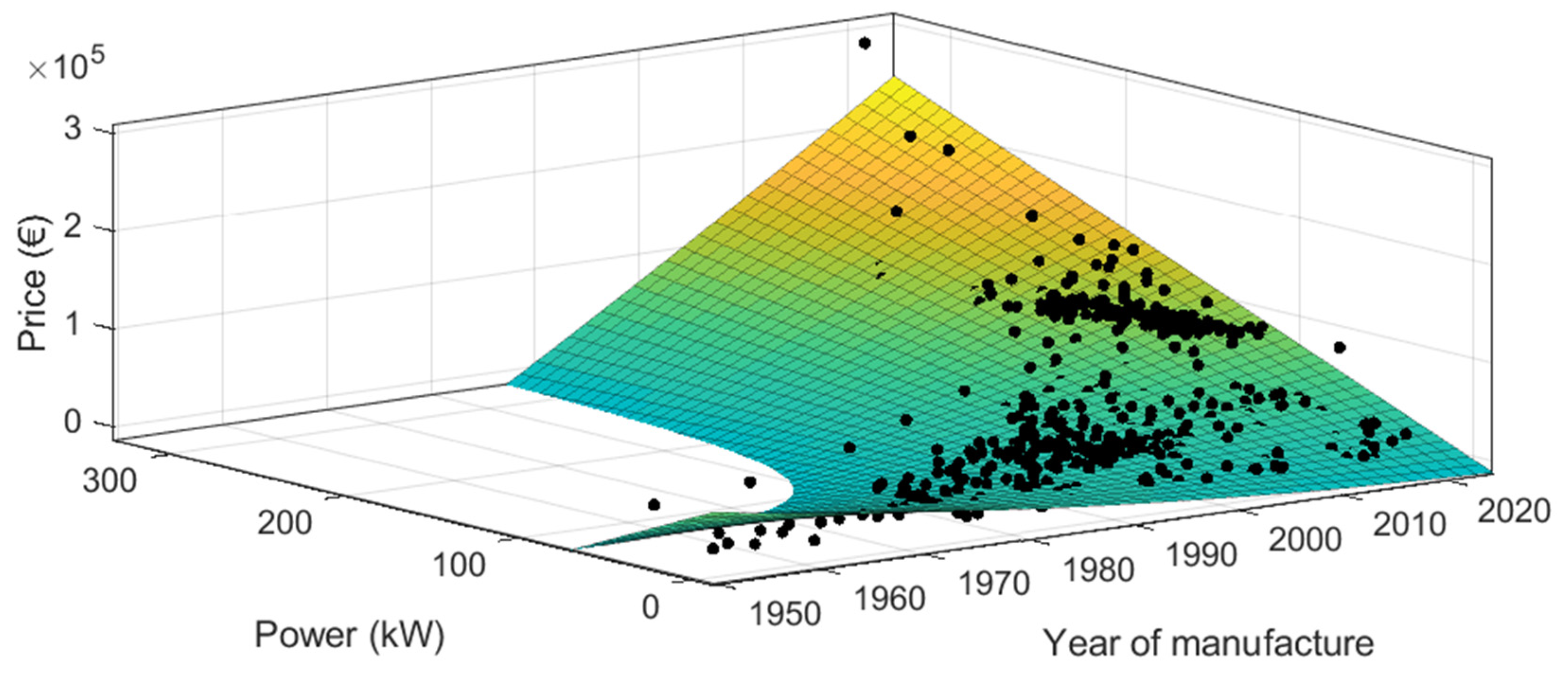
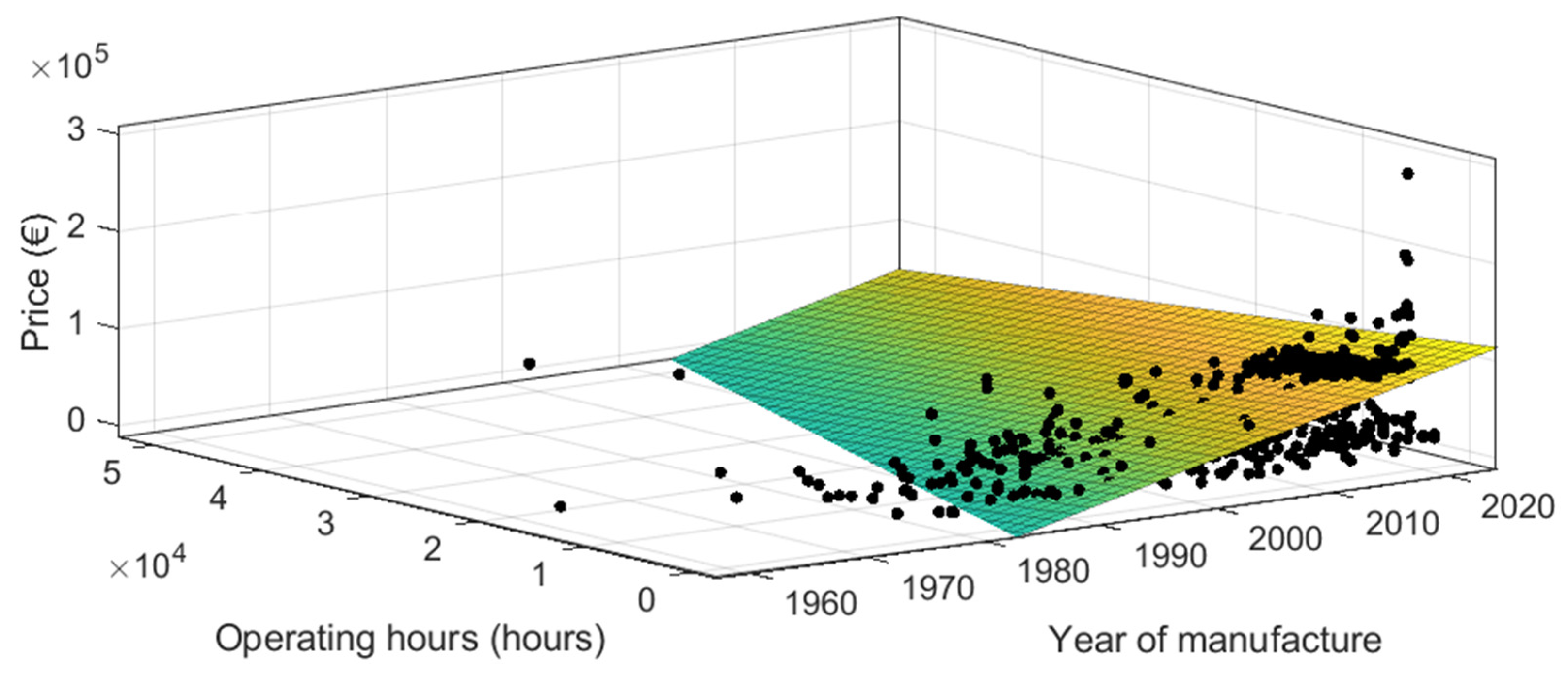
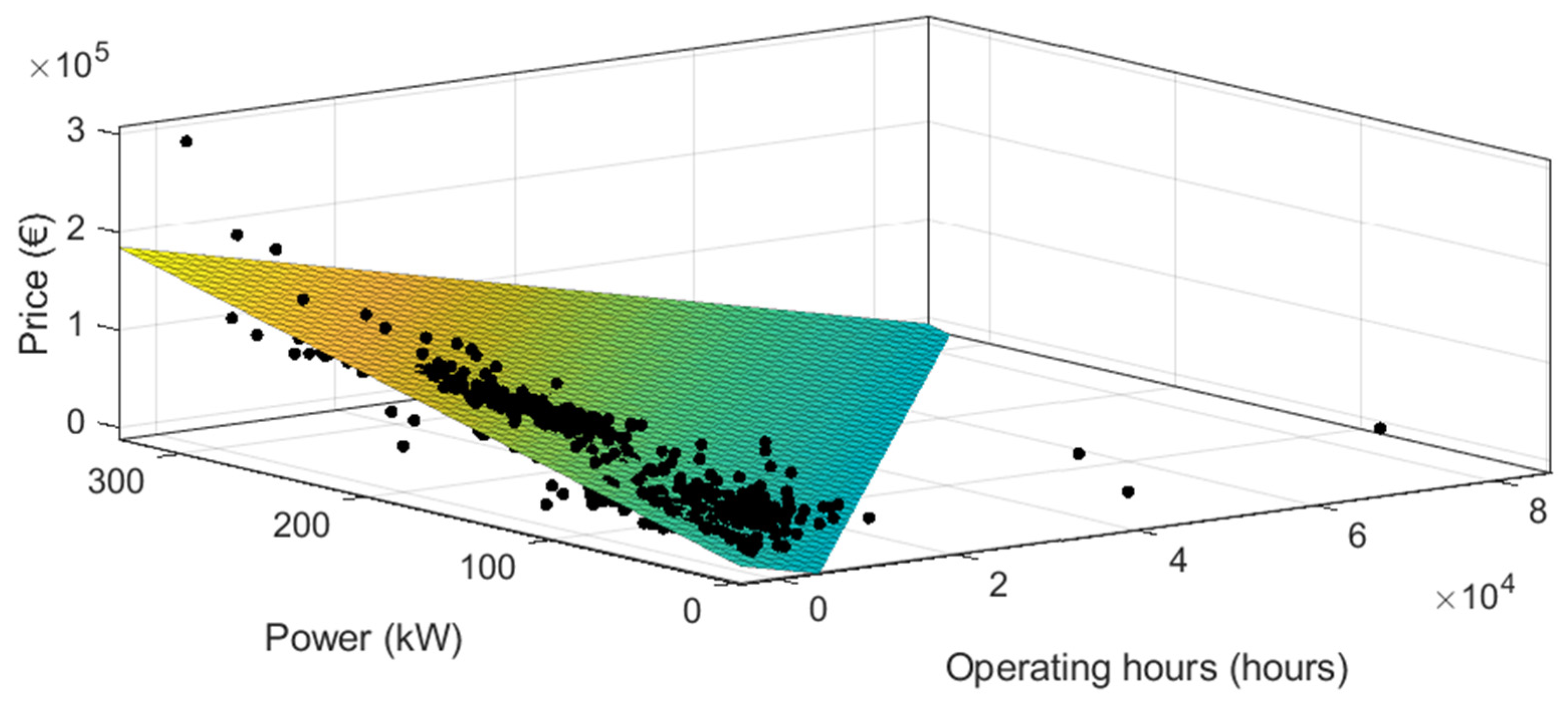
3.2.1. Taking Variables 2 by 2 with the Whole Second-Hand Tractor Dataset

With the whole dataset of second-hand tractors, the results show that it is possible to predict the price of second-hand tractors with different combinations of the three predictor variables 2 by 2 (see Figure 21, Figure 22 and Figure 23, and

Table 10. Summary of results with the whole dataset of second-hand tractors, taking variables 2 by 2.

Dependent Variable	Independent Variables	Model Type	Adjusted R2
Price	Operating hours, power	Polynomial model degree 1	0.9912
Price	Year of manufacture, power	Polynomial model degree 2	0.9927
Price	Year of manufacture, operating hours	Polynomial model degree 1	0.9893

). The best adjusted R² was achieved when using year of manufacture and power as predictor variables (adjusted R² = 0.9927) but were very close to the results of “operating hours and power” (adjusted R² = 0.9912).

3.2.2. Segmentation by Brand

In the case of second-hand tractors, price data were obtained for the following brands: Agria, Antonio Carraro, Arbos, Astoa, BCS, Belarus, Benassi, Case Ih, Caterpillar, Claas, Deutz-Fahr, Ebro, Fendt, Fiat, Ford, Goldoni, Hurlimann, JCB, John Deere, Kioti, Kubota, Lamborghini, Lander, Landini, Massey Ferguson, Mc Cormick, Mercedes-Benz, New Holland, Pasquali, Renault, Same, Sava Nuffield, Solis, Steyr, Valtra, White, Zetor.

Linear robust regressions were performed, using different combinations of predictor variables, for the brands with the largest amount of data. These were the brands: Case IH, Claas, Deutz-Fahr, Fendt, Fiat, John Deere, Massey Ferguson, New Holland and Same.

Doing a segmentation by brand, it is possible to get good and more specific adjustments, in most cases (see

Table 11. Summary of results performing segmentation by brand in second-hand tractors.

Brand	Data Number	Dependent Variable	Independent Variables	Polynomial Degree	Adjusted R2
CASE IH	57	Price	Operating hours, power	1	0.8896
			Year of manufacture, power	1	0.8836
			Year of manufacture, operating hours, power	2	0.9512
CLAAS	54	Price	Operating hours, power	1	0.9232
			Year of manufacture, power	1	0.9195
			Year of manufacture, operating hours, power	2	0.7840
DEUTZ-FAHR	24	Price	Operating hours, power	5	0.8530
			Year of manufacture, power	5	1
			Year of manufacture, operating hours, power	2	0.9569
FENDT	107	Price	Operating hours, power	1	0.9576
			Year of manufacture, power	1	0.9676
			Year of manufacture, operating hours, power	2	0.8246
FIAT	37	Price	Operating hours, power	1	0.7886
			Year of manufacture, power	2	0.7048
			Year of manufacture, operating hours, power	2	0.667
JOHN DEERE	275	Price	Operating hours, power	5	0.8289
			Year of manufacture, power	5	0.8400
			Year of manufacture, operating hours, power	2	0.8574
MASSEY FERGUSON	86	Price	Operating hours, power	5	0.9263
			Year of manufacture, power	5	0.8937
			Year of manufacture, operating hours, power	2	0.9472
NEW HOLLAND	99	Price	Operating hours, power	1	0.9459
			Year of manufacture, power	1	0.9511
			Year of manufacture, operating hours, power	2	0.746
SAME	34	Price	Operating hours, power	4	0.6882
			Year of manufacture, power	1	0.3600
			Year of manufacture, operating hours, power	1	0.6855

).

In the analyses with 2 predictor variables, it is possible to make 3D figures, which allows to monitor the fit of the polynomial to the data and to use polynomials of higher degree. In the analyses with three predictor variables, only first and second order polynomials were used, in order to avoid abuse of regression analysis.

3.2.3. Segmentation by Power Range

In the power range segmentation, robust multiple regressions were performed taking variables 2 by 2 and with the three ones. The results were mixed. However, in every power range always the best results came from using “operating hours and power” and “year of manufacture and power”. Always these two combinations are the best (see

Table 12. Summary of results for segmentation by power range in second-hand tractors.

Power (kW)	Data Number	Dependent Variable	Independent Variables	Polynomial Degree	Adjusted R2
0–50	193	Price	Operating hours, power	1	0.8917
			Year of manufacture, power	1	0.9397
			Operating hours, year of manufacture	1	0.8813
			Year of manufacture, operating hours, power	1	0.3520
51–150	626	Price	Operating hours, power	1	0.9897
			Year of manufacture, power	1	0.9907
			Operating hours, year of manufacture	1	0.4298
			Year of manufacture, operating hours, power	1	0.8577
151–250	162	Price	Operating hours, power	1	0.9694
			Year of manufacture, power	1	0.9794
			Operating hours, year of manufacture	1	0.9742
			Year of manufacture, operating hours, power	1	0.6400
More than 250	22	Price	Operating hours, power	1	0.8947
			Year of manufacture, power	1	0.8442
			Operating hours, year of manufacture	1	0.7297
			Year of manufacture, operating hours, power	2	0.7665

).

On the other hand, when using “Operating hours and year of manufacture” and “Year of manufacture, operating hours and power” the results are worse.

3.2.4. Segmentation by Category

Of the official categories into which MAPA classifies, enough data numbers were only available for the following categories:

• Crawler Tractors
• 4WD Narrow and Articulated Tractor
• 4WD Narrow Tractor
• 4WD Normal Width Tractor
• 2WD Narrow Tractor
• 2WD Normal Width Tractor

In these analysis, the adjusted R² were very good, most of them greater than 0.9. The highest adjusted R² were obtained always when 2 predictor variables were used. The lowest adjusted R² were obtained when 3 predictor variables were used (see

Table 13. Summary of results performing segmentation by official category in second-hand tractors.

Categories	Data Number	Dependent Variable	Independent Variables	Polynomial Degree	Adjusted R2
4WD Narrow and Articulated Tractor	28	Price	Operating hours, power	3	1
			Year of manufacture, power	4	0.9767
			Year of manufacture, operating hours, power	1	0.9100
4WD Narrow Tractors	124	Price	Operating hours, power	1	0.9308
			Year of manufacture, power	1	0.9384
			Year of manufacture, operating hours, power	2	0.653
4WD Normal Width Tractors	653	Price	Operating hours, power	1	0.9910
			Year of manufacture, power	1	0.9916
			Year of manufacture, operating hours, power	1	0.7300
2WD Narrow Tractors	26	Price	Operating hours, power	5	0.9929
			Year of manufacture, power	4	0.7589
			Year of manufacture, operating hours, power	2	0.7880
2WD Normal Width Tractors	155	Price	Operating hours, power	1	0.8796
			Year of manufacture, power	1	0.9320
			Year of manufacture, operating hours, power	2	0.6990

).

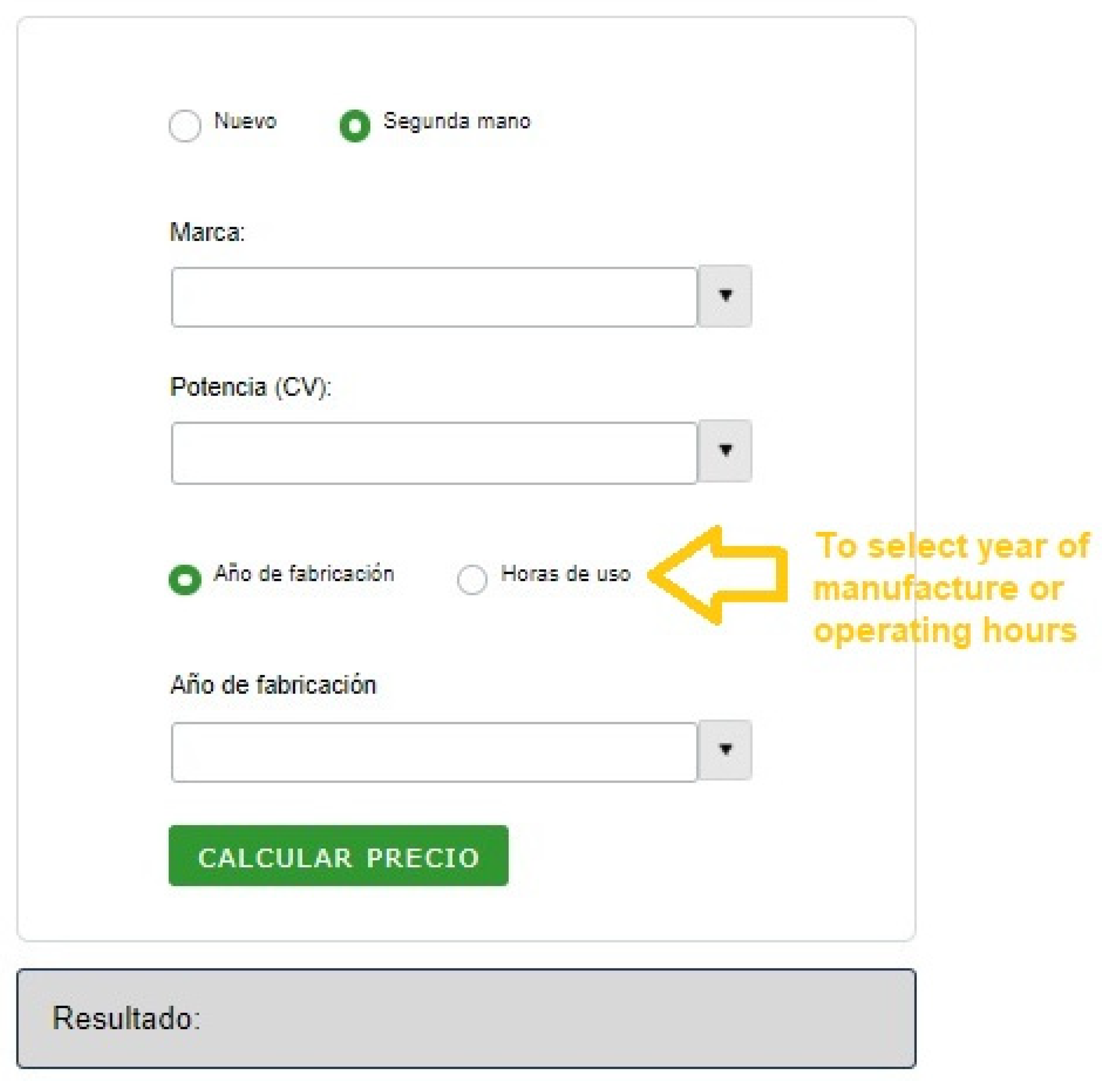
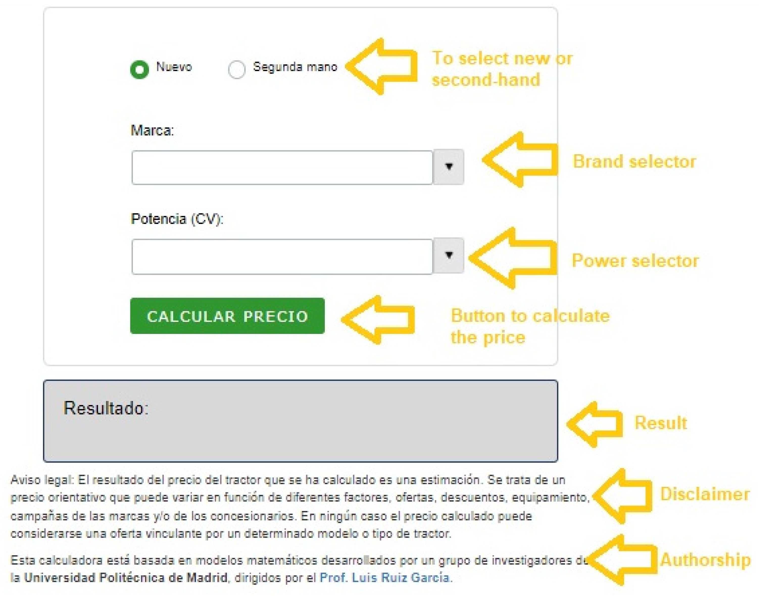
3.3. Decision Support Tool

The decision support tool is available and fully operative at: https://www.tractoresymaquinas.com/calculadora-precios-tractores/ (see Figure 24 and Figure 25). It is an open and free tool, very easy to use. It is done in a web environment, but it can be also implemented in a smartphone APP for Android or IOS. It is in Spanish because it is implemented in a Spanish site dedicated to tractors and other farm machinery. The number of fields and options were reduced to a minimum, with the idea of making the tool as simple as possible.

In the first place, the user must choose between new and used. If he chooses “new” then he will have to select brand and power. The power selector uses CV for power units, because it is the most commonly used unit by the farmers in Spain. Pressing the button of calculate price, one will get an estimation of the price of the tractor based on the mathematical models developed in this study (see Figure 24). For each brand, there is a specific range of power.

If one chooses second-hand, the user can also select year of manufacture or operating hours (see Figure 25). For each brand, there are also specific ranges of year of manufacture and operating hours.

The interface includes a disclaimer and information about the authorship of the tool, in order to build user confidence. Moreover, each time the tool is used, the inputs and the output are saved in a database. This gives feedback about the performance of the models and the search needs of the users.

4. Discussion

Farm tractors have many different characteristics (brand, dimensions, power, displacement, gearbox, transmission, steering, hydraulics, roll over protection systems, etc.). However, with just a few of these variables, we can predict their price.

Regarding new tractors, this study is in line with the study of tractors in Italy and Spain, in which it is said that the price of new tractors can be modeled using only power as predictor variable. In that study the variance explained was 89% in Spain and 73% in Italy, and in this study, it is 99.81% using a robust LAR adjustment [34,41].

Segmentations by brand, with the data of new tractors, have also given good results and more specific predictions than the analysis of the whole dataset of new tractors. This has not been the case with the segmentations by category and by power range, where the results have been worse than that with the whole new tractor dataset.

In the case of predicting used tractor prices, the results showed that it is possible to predict the price of second-hand tractors, with very good precision, doing robust linear regressions with only three predictor variables (power, year of manufacture and operating hours) or taking 2 by 2. The use of short number of variables, reduces the risk of overfitting [42,45].

Predictive analytics with the whole dataset of the used tractors, using these three predictor variables, achieved 88.70% of explained variance, which is similar to the result from another study done with a dataset from UK [37]. Using only power and age, the result is 99.27% of explained variance, which is higher than the 73.4% achieved in a previous study [34].

In second-hand tractors, doing segmentations by brand, power range, and category it is also possible to achieve better results, with adjusted R² > 0.9 in most cases, using variables 2 by 2.

Regarding the type of parametric models, in the present study, all the models obtained for estimating the market value of tractor were polynomic. However, previous studies found better results with logarithmic-linear types [33,41,46,47] or cubic [37].

In previous studies, some variables like brand or traction, were considered binary variables, with the aim to do one model for new and another one for second-hand tractors [34,37,41]. Doing segmentations by brand, horsepower or type, like in this study, allows the development of more precise mathematical models that provide better predictions. This new approach improves the performance of the DST.

Regarding non-parametric models, for new and second-hand tractors datasets, the non-parametric regression models tested (regression trees, support vector machines, ensembles of regression trees, Gaussian process, and Neural Networks) do not provide better results than robust linear regressions. Those more complex models were not tested by previous studies [30,31,32,33,34,35,37,38,39,41,48], but there is no additional benefit to be gained by choosing them.

The DST developed in the present study has the three fundamental characteristics that any DST should have: a database that can store and manage internal and external information, algorithms necessary for the analysis, and an interface for communication with the user [12].

The present DST fulfills the eight core factors that influence the uptake and use of DST by farmers, established by Rose et al., 2016. These factors are performance expectancy, easy to use, peer recommendation, trust, cost, habit, relevance to user and farmer-adviser compatibility [20].

Regarding performance, this DST works efficiently, provides up-to-date information, give accurate predictions or information, and enable better decision-making. DST is very easy to use because it provides information in a quick, user-friendly way, works in any browser, has a clear and simple design with only few options for the inputs and one clear output. The peer recommendation is not extensive because it is a DST that has just been launched. But if the DST performs well, the peer recommendation will come.

Regarding trust, farmers and advisers are keen to use tools from trusted sources. For this reason, there is a text in the bottom of the DST saying that it is a neutral decision support tool based on algorithm done by a public university, not a farm machinery manufacturer, dealer, or distributor. Thus, it is something that farmers can trust. This DST is also free to use. Users do not have to pay and can use the DST for an unlimited number of times.

In the case of habit, younger farmers are used to using computers and smartphones. They will seamlessly start to use a decision support tool delivered in the form of software or apps. Following this approach, the present DST can be used in any smartphone, tablet, or computer. It works in a www secured environment.

Regarding the relevance to user, this DST is sufficiently flexible to serve the needs of an individual but it is also generic. It gives specific results for the most popular brands, but also has general models that can be applied to any brand.

In this DST the farmer-adviser compatibility is guaranteed, because it is accessible for both and is compatible with any browser or Internet device.

5. Conclusions

With the parametric models developed in this study, a calculator for estimating new and used tractor prices was developed, implemented, test, and validated. This calculator is currently used as a decision support tool for buying and selling tractors. This tool can lead users through clear steps and suggest optimal decision paths in the process of buying farm tractors.

This tool saves time and money to farmers and machine dealers. In the case of new tractors, the farmer does not need to visit several stores to get a price information. He just can use the tool and get many different price estimations in a short time. For the machine dealers, it is a very easy way to compare tractor prices of different brands. In the case of second-hand tractors, the tool summarizes and condenses the information of thousands of tractors models with different characteristics, operating hours, and age (year of manufacture).

Moreover, the DST has other benefits. To the buyer, the farmer, it allows to detect fraudulent offers, suspicious for being too cheap or too expensive. The seller or tractor owner can estimate the remaining value of his tractor or the selling price in the market. The seller does not need to be an expert appraiser to know how much to sell his used tractors for.