1. Introduction
Conventional pig farmers, who produce nearly homogeneous pigs in terms of body weight and composition, are particularly exposed to strong international competition and affected by an increasingly poor market situation. This leads to low market power on the part of producers and consequently low market performance [
1]. Producers are encouraged to reduce unit production costs as much as possible by increasing production volumes (economies of scale). This is the main reason for the structural change in pork production in recent years, which has moved away from many smaller farms towards fewer—but larger and more specialised—farms [
2,
3].
However, this development also leads to a greater distance between the fattener and the individual animal in terms of less time per animal [
4]. In light of the trend of keeping “masses of animals” without precise knowledge about individual animals, an individual animal identification (IAI) system represents an option in the context of precision livestock farming [
5].
IAI enables the collection of data on individual animals, which can ensure full traceability and thus strengthen the trust of consumers (“from stable to table”; [
6]). Such data are also used for animal welfare monitoring [
7] and management decisions such as individual feeding [
8] or optimised slaughter deliveries [
9,
10]. Thus, individual animal data provide the basis for improved animal welfare, lower emissions, and improved performance, which enables a production that is favourable in terms of its costs and appropriate to the animal species [
11].
To date, IAI has mainly been used in research and breeding, where the most accurate data are required [
12]. In conventional pig fattening, permanent IAI is not yet common, since the costs involved and the added value for the fattener have not yet been determined [
13].
In addition to analogue identification, there is also electronic or digital identification. Transponders are either implanted into the animal’s body or placed on collars or ear tags [
14,
15]. Collars are not a practical option for pigs due to anatomical reasons (short neck with little separation from the head) [
16].
Furthermore, the required working time is also a decisive factor. According to Rau [
17], marking a litter with the ear tag required by law and a supplementary ear tag takes a total of 19.62 min per litter (10 piglets per litter; 1.96 min per piglet) with three workers. In contrast, the time required to mark and document a pig using an ear tag, where the front side is in accordance with the legal requirements (analogue) and the back side is the transponder, is estimated at an additional 3 min per litter (0.3 min per piglet) when compared to the standard ear tag. However, this only applies to marking on the third day of life. From the 14th day onwards, an estimated 6.18 min per litter (0.618 min per piglet) is required [
17].
The minimum equipment required for the use of digital IAI is an ear tag transponder and reader with software. The cost of equipping a barn for fattening pigs with IAI technology (i.e., UHF RFID readers at troughs, drinkers, and barn ramps) was calculated at EUR 11.70/animal space for 1600 fattening places for the initial installation and at EUR 7.60/animal space for an identical number of animals in subsequent runs [
18]. With an average output and 2.85 turnovers per year [
19], this corresponds to costs of EUR 4.11 and EUR 2.66 per pig, respectively. The greatest obstacle to the widespread implementation and greatest associated benefit of transponders in a barn is the animal owners themselves. They must first be sufficiently trained so that they are interested in receiving as much data as possible [
20]. Additionally, mechanical barn equipment (e.g., scales) are susceptible to malfunctions due to dirt, dust, and faecal deposits [
21].
In contrast, the use of UHF RFID ear tags with the automatic registration of animals at troughs and drinkers results in a potential savings of up to EUR 1.10/animal in barns with 400 pigs and EUR 1.00 per animal in barns with 1600 pigs, through early disease detection and more efficient animal control. This is based on calculated annual medical and veterinary costs of EUR 4.30 and EUR 2.60 per animal (based on 400 and 1600 fattening places, respectively) and calculated annual labour costs for animal control per fattening place and year of 0.3 and 0.5 h (based on 400 and 1600 fattening places, respectively) at 2.85 rotations [
11].
This work aims to highlight the practical suitability of IAI using transponder ear tags in conventional pig fattening while simultaneously presenting possible applications that make IAI economically attractive.
Therefore, the use of IAI via UHF RFID transponder ear tags in fattening pigs was evaluated under field conditions in the present study. Notably, a decline in unit production costs by using IAI was demonstrated. For this purpose, data on individual animals were collected during the suckling and fattening stages and different selection scenarios were carried out to investigate its use from an economic perspective.
The relevance of this study for the entire supply chain is also underpinned by the fact that one of the largest food retailers in Germany will only sell fresh pork produced in Germany (birth, rearing, fattening, slaughter, and cutting/processing) by the end of 2022 [
22]. This shows that the interest in data on the origin of the animals to be slaughtered is also becoming of increasing interest in conventional farming. Being able to track or provide data for each pig would be another way to add value to the product.
2. Materials and Methods
One-day-old, crossbred piglets (Danbred F1 (Landrace × Yorkshire) × Pietrain (BHZP db.77®); n = 304) were marked individually. This number of piglets included a buffer of 80 additional animals to ensure that 224 pigs of the same age were available in the fattening unit.
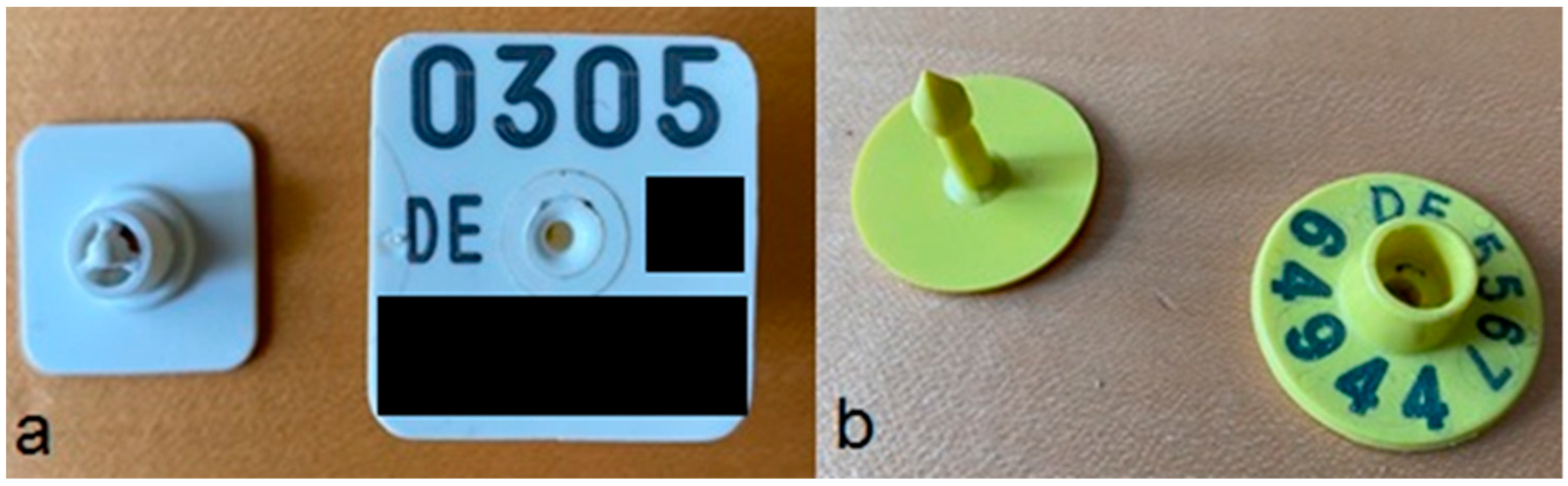
For individual animal identification, two different ear tags were used (see
Figure 1). The analogue ear tag (Merko M2, Allflex, Bad Bentheim, Germany; 30 × 30 mm, 1 mm thickness) was square and numbered from 001 to 304. Additionally, the farm number of the producer was printed on it in accordance with regulations. The electronic ear tag transponder (MS Tag Round UHF Standard, MS Schippers, Kerken, Germany; 26 mm diameter, 2 mm thickness) was attached to the other ear. As a distinguishing visual feature, the last five digits of the individual number were printed on the ear tags. With a length of approximately 2 cm and a width of 4 mm, the spines of the ear tags did not differ. A Motorola Psion Workabout Pro4 handheld reader (Motorola Mobility, Libertyville, USA; Windows operating system) with the software d!ba Mobile (definitiv! business applications, Münster, Germany) was used to communicate with the transponders.
The fattening unit used in this study was a closed, thermally insulated, forcibly ventilated double comb unit (“Bünne Swine Center”) with paved aisles and fully slatted pens. In addition to a dry mash feeder (four feeding places) with two drinking bowls, each pen also contained two drinking nipples at different heights. City water was used, which was preheated to 18 °C. The pen size without a feeder was 10.5 m
2 (0.75 m
2 per pig). The piglets were randomly allocated to 16 pens (
n = 14 in each) and separated by sex. All pigs were treated the same. Three commercial compound feeds were provided to pigs during the trial. The botanical composition of the feed is provided in
Table 1.
Analyses of chemical composition were performed according to standard laboratory methods (nutrients: proximate analysis; fibre analysis: van Soest; minerals: atomic ab-sorption spectrometry after acid hydrolysis; amino acids: after acid hydrolysis using HPLC [
23]). The chemical composition is presented in
Table 1. The energy content was calculated using the following formula: ME (MJ/kg) = 0.021503 × crude protein (g/kg) + 0.032497 × crude fat (g/kg)—0.021071 × crude fibre + 0.016309 × starch (g/kg) + 0.014701 × organic residue (g/kg) [
24].
By using a pneumatic multi-phase feeder (Schauer Spotmix, SCHAUER Agrotronic, Prambachkirchen, Austria), each feeder was filled individually. Since all animals were fed the same feed in the trial, only the quantity per pen varied. At the time of the feed change, the new feed was not mixed to achieve a concrete weighing time. The feed changes were determined according to the average amount of feed already consumed, whereby a total feed consumption of 250 kg per pig was calculated (80 kg pre-fattening/grower, 50 kg mid-fattening/grower-finisher, 120 kg final fattening/finisher).
Fresh feed was added daily at two fixed times (07:00 and 14:30). The exact feed consumption was recorded electronically for each feed trough. The fill level of the pen-specific feeders was recorded manually every day and then adjusted in the feeding software such that the feeder was emptied after each feeding. Regarding feed consumption, it was assumed that the consumption of each pig per pen was identical. In pens where animals were eliminated within a phase, the total feed consumption per pen was calculated by subtracting the consumption of the eliminated animal from the total feed consumption. A reduction of half the feed compared to the pen mean was assumed by the time they were eliminated.
During fattening, individual weighings were performed nine times by two people. For this purpose, the pigs were driven bay by bay to the drive aisle. From there, each animal was weighed individually on a low-floor animal scale. Furthermore, ear tag losses and the time taken for the work involved were recorded. To ensure full traceability before each delivery, the abattoir was informed in writing that fattening pigs were delivered with ear tag transponders to determine the proportion of pigs automatically registered using an electronic ear tag. Ear tag or transponder losses during transport were not recorded.
Primarily, we analysed the fattening performance data for each phase (daily weight gain, average feed intake). The assumption of normally distributed data was tested using the Kolmogorov–Smirnov and Shapiro–Wilk tests. The equality of variances was tested using Levene’s test.
With the homogeneity of variances and normally distributed values, the mean values for the fattening performance parameters per sex were compared by two-sample t-tests for independent samples. Only mean values from the same period were compared. Provided a significance level of p ≤ 0.05, the results could be considered statistically significant. In total, there were three scenarios with eight selections each, which were based on live weight and sex. All pigs whose body weight at the selected time deviated by more than 10, 15, or 20% from the calculated mean value of the initial group were removed from the data set, while the remaining animals were considered part of a newly selected group. Each of the three scenarios (10, 15, and 20%, respectively) were divided into eight further selection groups (S) based on the age (in days) of the pigs at the time of selection (S77, S119, S138, S151, S161, S174, and S182). To facilitate the respective allocation, the selection intensity parameter was always assigned to the selection group. For example, the marking “S161/15%” implies that the pig was selected to M—15% on the 161st day of life. Until this selection, the records of the selection group corresponded to those of the initial group. Selections were not made after the 182nd day since the number of remaining pigs was no longer sufficient for further selection at that point. A special scenario was the selection at each weighing time, abbreviated as SEP (E = each, P = phase) henceforth. The extraction of data sets based on the selection criteria resulted in changes in the fattening performance data.
To evaluate the scenarios from an economic perspective, two different approaches were carried out, whereby female animals and castrates were considered separately. Notably, the calculations are presented in a simplified form based on partial costing. The first approach was the economic evaluation of different fattening times for the selection groups. Here, the daily difference in average fattening duration was calculated and multiplied by the direct costs incurred for a final fattening day. The following parameters were assumed for this procedure: The finisher diet costs EUR 21 per 100 kg (actual situation at the time of the trial, calculated as the arithmetic mean of the previous 3 months) and an average of 3.0 kg per pig per day is provided. This resulted in daily feed costs of EUR 0.63 per pig. Additionally, there were daily costs for veterinarians, energy, water, and other expenses of EUR 0.08 per pig. Furthermore, liquid manure disposal was estimated at EUR 14.00 per m3 (actual situation at the time of the trial, calculated as the arithmetic mean of the previous 3 months), whereby each pig produces 0.40 m³ of liquid manure during the entire fattening period (the actual situation was measured by a flow pump). Under the condition that the same amount of liquid manure was produced on each fattening day, an amount of EUR 0.056 per fattening day (14/0.4 m3/100 days) results if 100 fattening days are defined. In total, this resulted in comparable direct costs of EUR 0.766 per final fattening day per pig.
The second approach compared the feed costs of the selection groups for each kilogram of live gain based on individual pig data, as measured during fattening. This is shown as the quotient of the total feed costs and the total gain per selection group (in EUR). To calculate the feed costs, the average daily feed intake was multiplied by the duration of the phase (in days) and the feed price at the time of the phase. The feed price was set at EUR 0.25 per kg for pre-fattening, EUR 0.23 per kg for mid-fattening, and EUR 0.21 per kg from final fattening onwards (actual situation at the time of the trial, calculated as the arithmetic mean of the previous 3 months). The product of the individual phase was used as a summand for the entire fattening to form the final sum. The total gain of each selection group was calculated by summing all products from the mean daily gain and the duration of the individual phases (in days).
While the approach with the reduced direct costs referred to the entire fattening period from housing to slaughter, the second approach only considered the six fattening phases up to and including the phase of the third removal from the pen.
3. Results
The suckling period was 26 days, and the subsequent piglet rearing period was 51 days. Fattening was divided into six phases of different lengths (see
Table 2), with pre-fattening lasting 42 days, mid-fattening 18 days, and finishing 12 days. The final fattening phase was followed by the housing out phases, which lasted 9, 12, and 7 days, respectively (marked 1–3 in
Table 2).
In this section, the fattening performance data calculated for each phase and sex are presented using the arithmetic mean (M) with standard deviation (SD) and the lowest and highest values of the data set in the following format: M ± SD (min–max). In the pre-fattening phase, the feed intake (as fed) of the females was 1.94 ± 0.09 kg, while that of the castrates was 2.10 ± 0.14 kg (+8.45%). While the feed intake of the females increased continuously and reached its highest value (3.02 ± 0.15 kg) at the end of fattening in phase six, the values for the castrates were already lower in phase five (3.38 ± 0.24 kg) than previously in phase four (3.43 ± 0.17 kg). Nevertheless, the highest value of 3.53 ± 0.23 kg was also reached by the castrates at the end of fattening in phase six (see
Table 3).
In all phases, there was high heterogeneity within the groups. For example, the feed intake of the castrates in the pre-fattening phase varied between 1.89 and 2.38 kg/animal/day, which corresponds to a difference of 490 g per day. Another example is the female animals in phase four, whose daily feed consumption per animal was 2.76 to 3.20 kg, which corresponds to a difference of 440 g per day.
On the day of farrowing (d 1), the weights of the total sample varied between 0.64 and 2.56 kg (+300%) (see
Table 4). On average, male piglets were 70 g (+4.86%) heavier than females. The SD of birth weight was 0.35 kg for females and 0.36 kg for males, which corresponds to 24.3 and 23.8% of the mean value, respectively. At weaning on the 26th day of life, the females were 20 g (+0.26%) heavier than the castrates, with an average of 7.79 ± 1.75 kg. At this stage, there were already weight differences between the sexes. The smallest female weighed 2.69 kg and the heaviest was 11.5 kg (+327%). In the case of the castrates, weights ranged from 3.97 to 11.2 kg (+182%).
At housing to fattening (77th day of life), 112 females (32.3 ± 6.25 kg) and 112 castrates (32.2 ± 6.38 kg) were placed in the fattening house. Irrespective of sex, the body masses of all animals at this time varied between 18 and 47 kg (+161%). No significant differences in the live weights of the sexes were observed up to and including the time of housing out.
The first housing out took place on the 151st day of life, immediately after the determination of individual body masses. At that time, the body masses of females varied between 68 and 124 kg (+82.4%) and between 85 and 130 kg (+52.9%) for castrates. The heaviest eight females and 20 castrates (with a live mass of at least 114 kg) were removed (see
Table 5). Up to and including the 161st day of life, the weights of the castrates were significantly higher than those of the females. Weights differed weakly within the sexes at the 119th day of life. Thereafter, weights differed strongly and significantly at the ages of 138, 151, and 161 days (
p < 0.01). The measured differences were 2.6 kg (+3.68%) on the 119th day of life, 4.7 kg (+5.38%) on the 138th day of life, 5.0 kg (+5.00%) on the 151st day of life, and 4.0 kg (+3.70%) on the 161st day of life. In the following period, the castrates were always slightly heavier than the females at their respective slaughter dates. While the last castrate was slaughtered on its 199th day of life at 126 kg, the five remaining females were slaughtered on the 210th day of life at 116 ± 8.75 kg (range: 102–128 kg).
There were highly significant correlations between age at slaughter and birth, weaning, and housing to fattening age weight.
The daily gains of the castrates were significantly higher than those of the female pigs in the first four phases (see
Table 6). In the latter phases, they increased from 0.920 ± 0.10 kg at pre-fattening (phase one) to a maximum of 1.035 ± 0.26 kg in phase four. In the case of the castrates, daily gains of 0.971 ± 0.11 kg were already achieved in pre-fattening. The highest value (1.198 ± 0.43 kg) was observed in phase four. In both female pigs and castrates, the daily gains in phase five fell back to values below 1 kg. Although the daily gain among females in phase six continued to decrease to 0.906 ± 0.32 kg, it increased to 1.062 ± 0.18 kg among the castrates. The large variation in daily gains was also striking in both females and castrates. This became especially clear in phase four. In this phase, there were pigs (both females and castrates) that lost weight (−0.2 and −0.8 kg, respectively). Simultaneously, the pigs with the highest calculated daily gains—1.78 kg among the female pigs and 1.56 kg among the castrates—were also in this phase.
Table 7 presents the selection limits based on the individual live masses of the different sexes.
The average slaughter age of the females was 177 ± 13.4 (range: 151–210) days, which corresponds to approximately 100 fattening days. The initial group of castrates was slaughtered at an average of 169 ± 13.8 (range: 151–210) days. Thus, in contrast to the females, castrates had a fattening period that was slightly more than 8 days shorter (
p < 0.01; see
Table 8). Under the specified conditions, this led to a direct cost saving of EUR 6.13 per pig if the fattening place was occupied with a castrate and not with a female animal.
In contrast to the castrates, each selection scenario led to an earlier average slaughter date for the females. Among the females, the last and weakest selection group S182/20% resulted in a 0.32-day shorter fattening period and thus a direct cost savings of EUR 0.25 per pig. For castrates, the last animals in scenario S174/10% were covered by the selection and thus resulted in a savings of EUR 0.39 per pig. For the effective selection groups of castrates, the average lifetime varied between approximately 168 (S174/10%) and 162 days (SEP/10%), in which EUR 5.44 of direct costs could be saved per pig. For females, the average lifespan varied between approximately 171 (SEP/10%) and 177 days (S182/20%), resulting in a maximum cost savings of EUR 4.56. It is striking that selection with an intensity of 10% on the 119th day had less influence on both females and castrates than selection on the 138th day. Early selection with a high selection level tends to have a stronger impact than selection later in the fattening. Overall, the mean direct cost savings between females and castrates did not differ significantly.
Table 9 presents both the feed costs and gains in the individual selection groups. The mean cost per kg of gain was significantly lower (
p < 0.01) for females than for castrates.
Females (initial group) had a cost per kg of gain of EUR 0.573 (total feed cost of EUR 5658 and 9874 kg gain), while castrates (initial group) had a cost per kg of gain of EUR 0.596 (total feed cost of EUR 5868 and 9846 kg gain). The initial groups had both the highest feed costs and the highest total gains.
The lowest feed costs per kg of gain were observed for the castrates (SEP/10%) at EUR 0.581. This was followed by SEP/20% (EUR 0.582) and S138/10% (EUR 0.583). Among the females, the group with the lowest feed costs was the selection group S138/10% at EUR 0.562 per kg of gain. This was followed by S119/10% (EUR 0.565) and SEP/10% (EUR 0.565). Here, the feed costs per kg of gain were identical for both selection groups; however, the total feed costs and gains differed strongly, with S119/10% resulting in higher feed costs (EUR 1135). The respective scenarios resulted in a maximum reduction in costs of 1.1 cents (S138/10%) per kg of gain for females and 1.5 cents (SEP/10%) for castrates.
It is striking that for both the castrates and females, selection group S77/10% had higher feed costs per kg of gain than selection at the same time at the level of 15%. For the castrates, the selection group S161/10% led to the same costs with higher total gains (+2754 kg).
Compared to the castrates, it was not the selection SEP/10% but rather S138/10% that led to the most favourable feed costs per kg of gain for the females. The difference between these selection groups was 0.3 cents per kg of gain. For both sexes, the ranges of feed costs and gains were strikingly large. Castrates of the selection group SEP/10% had the lowest feed costs and gains (compared to the initial group, feed costs were reduced by EUR 2247, and total gains were reduced by EUR 3616). Among the females, the greatest deviations were observed in the selection group SEP/10% (EUR 2149 feed costs and 3664 kg total gains).
Out of 224 analogue and electronic ear tags, a total of 86 (38.4%) analogue and 15 (6.7%) electronic ear tags were torn out and could no longer be found in the pens. The proportion of ear tags no longer firmly attached to ears was 57 analogue (25.4%) and seven (3.1%) electronic ear tags (see
Table 10).
A total of 202 pigs were delivered to the slaughterhouse, of which 187 had a functioning electronic ear tag installed. Of these, 166 were automatically recorded and assigned at the slaughterhouse, which corresponds to a selection rate of 88.8%. It is not possible to know whether ear tags were lost during transportation to the slaughterhouse or during the slaughter process. Since the pigs were weighed and electronically evaluated immediately before transport, a defect in the ear tags can be ruled out.
Until the end of the selections, the fattening lasted 105 days, which corresponds to approximately 3.5 months. The trial required 304 ear tag transponders (EUR 0.48/ear tag transponder) and a handheld reader with compatible software (EUR 117.53/month). For applying ear tags (including data collection), 1.82 min per pig was required, which corresponds to a total of 9.22 h. In the fattening unit, a total of 1295 individual animal weighings were performed, which took approximately 1.27 min per pig, corresponding to a total of 27.41 h. With an assumed gross hourly wage of EUR 18, the total cost was EUR 1217.87. In relation to all initially marked animals (n = 304), this corresponds to EUR 4.06 per pig. When considering only the animals housed in the fattening pen (n = 224), a cost of EUR 5.44 per pig was incurred.
4. Discussion
The present study aimed to evaluate the use of IAI in fattening pigs under field conditions. A prerequisite for this is always the clear identifiability of animals, which is why ear tag losses should be kept as low as possible. In relation to all 224 housed in pigs, the total ear tag losses in this study were particularly high, with a total of 38.4% for the analogue ear tags compared to 6.7% for the ear tag transponders. Furthermore, an additional 25.4% of analogue ear tags and only 3.1% of transponders were no longer firmly in the ear. The results indicate that the rectangular analogue ear tags have a much poorer hold in the ear than the round electronic ones. Since the application of all ear tags was performed by the same person under the same conditions, differences in applying were ruled out. In contrast, loss rates of 44.9% for ear tag transponders and only approximately 1% for analogue tags were previously recorded [
25]. It is striking that in both the present study and a study by Caja et al. [
25] the larger ear tags were more prone to losses. This suggests that losses are not necessarily related to the type of ear tag, but rather to its size, texture, and colour. This opinion is supported by several studies [
17,
26,
27]. In summary, it can be assumed that the analogue, white, and rectangular ear tags have a stronger appeal to pigs than the electronic, yellow, and round transponders. It should be critically noted that all ear tags in the trial were applied on the first day of life. Of all the losses of ear tags applied on the first and 14th day of life, 79% of all lost ear tags were applied on the first day of life [
17]. Moreover, the results indicate that with higher age, the relative ear tag losses increase. It must be considered that pigs with high growth performance were selected for the trial. The losses would likely be even higher among pigs that grow less rapidly and thus reach slaughter weight later in life. Thus, the risk of loss for the farmer increases with every day the pigs are kept longer in a barn.
Therefore, in future studies, analogue ear tags or transponders that are as small and inconspicuous as possible should be selected. Furthermore, data collection from the first day of life should be dispensed with in favour of better ear tag retention over the course of a pig’s life, which is made possible by ear tag collection at a later stage.
One problem that is not apparent from the results, but nevertheless causes problems, is the electronic registration of individual animals. It is possible that the desired transponder is not recorded, with another one being recorded instead. Even separation on animal scales does not reliably prevent false scans. It is possible that animals standing alone on a scale for individual weighing can be scanned as another animal, despite the other animals being more than one metre away. Notably, in contrast to low-frequency technology, UHF technology allows multiple scans of different transponders over a greater distance [
28]. If half-duplex system (HDX) or full-duplex system (FDX) transponders are used, these errors might not occur.
The results indicate that only 88.8% of the animals delivered with functioning ear tag transponders were automatically registered at the slaughterhouse and assigned to a carcass. This is not a satisfactory result on which to rely. It should be noted that small proportions of ear tags are also lost during transport to the slaughterhouse or at the slaughterhouse [
25,
29,
30], which was not recorded in the trial.
Regarding zootechnical parameters, the results of the study show that the average feed intake of the castrates in the trial was always significantly higher than that of the females. This illustrates the different nutritional needs of the individual animals [
24]. In the future, three models are conceivable for more targeted feeding. One possibility is to regularly form new groups, which is associated with stress and increased aggression in the animals [
31]. The second possibility is to register the animals individually at a sorting gate (“sensor-controlled digitisation in the barn”) and to direct them to an appropriate feeding pen with the right feed, which then leads back to the large group. The most modern—but also most demanding—variant is to mix an individual ration for each animal according to its current needs. Coupled with multi-phase feeding, this places high demands on management but also enables additional feed cost reductions of up to 10% [
32].
It has been shown that females grow more slowly during fattening and that they are unable to make up this difference over the fattening period and with increasing age when compared to castrates. This corresponds to the data of Shull [
33]. Consequently, if the marginal cost of growth at the end of fattening is higher than the marginal revenue, the farmer should consider the early culling of females to maximise profit. This was confirmed by Hilgers et al. [
34], who noted that higher slaughter weights can lead to reduced revenue per kilogram of carcass.
The delivery notes of the entry and exit weights of the study showed daily gains of 945 g for the regularly housed animals in this fattening cycle. The individual animal data showed individual values of up to 1.78 kg per day. The highest values occurred towards the end of the fattening period. Notably, the live weight (i.e., the basis for calculating weight gain) is influenced by the time of weighing during the day. As such, a pig weighed in the afternoon can be up to 1.5 kg heavier than when weighed in the morning [
35].
Selections Made during Fattening Based on Body Weight
The second objective was to demonstrate the economic savings potential of using IAI. Based on the premise of this research (i.e., that the savings per pig are linearly dependent on the difference in fattening days (EUR 0.766 per final fattening day, of which EUR 0.63 was for feed alone)), the highest savings were observed for the selection groups with the greatest reduction in average fattening duration. This was achieved through early and intensive selections.
As can already be assumed from the correlation between weight at the 77th day of life and age at slaughter (p < 0.01; r = −0.688), the selection S77/10% had a strong effect and resulted in an average savings of EUR 3.50 per female and EUR 4.36 per castrate. This implies that if only female animals or castrates had been housed, which had not been selected by S77/10% with age and weight, an amount of EUR 3.50 and EUR 4.36 per animal, respectively, would have been saved in fattening. With the number of animals housed in the trial of 112 animals each, this corresponds to EUR 392 for the females and EUR 488 for the castrates. In relation to the entire unit with a total of 1500 fattening places, savings of EUR 2625 and EUR 3270, respectively, would be achieved. It is particularly striking that in the case of the females, each selection led to a direct cost saving. Even selection on the 182nd day of life resulted in a savings of EUR 0.25 for the remaining animals. This situation was different for the castrates. Here, particularly late and weak selections did not result in any savings. Thus, under the observed conditions, a selection of female animals should always be considered. From an economic perspective, this implies that weak-growing females should not necessarily be fattened up to the target weight. Notably, this decision should be based on current feed costs and the market returns to be achieved. If feed costs and market revenues are high, early culling is particularly reasonable.
When calculating the sums of the feed costs for the growth of the selection groups based on the individual animal data, it became apparent that these hardly differ across all selection groups within the sexes. Although the total feed costs and weight increases varied greatly, the corresponding quotient was nearly the same. With a total increase of 90 kg as an example, a maximum difference of EUR 0.99 per fattening pig would result. Generally, the cost of this increase and the range of the selections tended to be EUR 0.596 to EUR 0.581 higher among the castrates; thus, a maximum difference of EUR 1.35 is given per castrate with an increase of 90 kg. Even if the difference seems small at approximately one euro each, this is an important potential saving when considering the large number of pigs fattened.
The result indicating that selection on only day 138 of life had the lowest feed costs per kg gain among female animals may be surprising. Even selection at each stage or at housing with 10% each had higher feed costs per kg of gain. Only selection at each stage was slightly cheaper than selection on the 138th day of life. It is striking that, in the calculation of costs, selection group S77/10% had slightly higher costs than selection group S151/10%. Therefore, early and strong selection is not always beneficial.
The relevance of possible savings for pig farmers becomes clear with slaughter prices of EUR 1.20 per kg of carcass weight in Germany in October 2021 [
36]. With a carcass weight of approximately 90 kg, this corresponds to revenue of approximately EUR 108, provided that no further deductions are made. After deducting direct costs for the purchased piglets and feed costs during fattening, most farms make a loss. Therefore, savings are an essential method for sustainable pig farming.
The new information gained from this study can now be used by farmers to place more targeted piglet orders (concerning growth potential) for their barns. When evaluating the results, it should be noted that the live masses of animals selected according to S77/10% were significantly higher at housing than that of the initial group. It is expected that the desired piglets are purchased at corresponding price premiums. These have a direct influence on the calculated savings. On the other hand, low-performing piglets would be offered at a lower price. Notably, the marketing of these piglets could be particularly difficult in times of surplus piglet supply. Consequently, it would no longer be in the producer’s interest to have as many weaned piglets as possible [
35]. Instead, healthy and vital piglets with a high market value would be preferred. Additionally, the reduction of litter size promotes higher piglet birth weight, which results in lower piglet mortality [
37].
5. Conclusions
In conclusion, based on individual data sets, this study has shown that IAI has enormous potential that can lead to high cost savings through targeted decisions.
Theoretically, the simplest way to individually identify pigs is by using ear tags (either analogue or digital). However, the study has shown that these do not have a sufficient hold; thus, high losses are possible. Therefore, this type of identification is not a practical option. Further studies should be performed to enable the more reliable and cost-effective identification of individual pigs.
As shown, it is unclear which selection intensity with which selection group makes the most economic sense for farmers. It has been shown that the selections allow enormous savings of up to about EUR 5.50 per animal. However, under selected circumstances, the cost of recording (EUR 4.06/pig) is too high; thus, most of these savings are lost. Nevertheless, further advantages can be expected from IAI, which will provide farmers with valuable information on the growth of piglets and additional added value through targeted marketing related to branded meat programmes.


