Impact of Camera Viewing Angle for Estimating Leaf Parameters of Wheat Plants from 3D Point Clouds

Abstract

Estimation of plant canopy using low-altitude imagery can help monitor the normal growth status of crops and is highly beneficial for various digital farming applications such as precision crop protection. However, extracting 3D canopy information from raw images requires studying the effect of sensor viewing angle by taking into accounts the limitations of the mobile platform routes inside the field. The main objective of this research was to estimate wheat (Triticum aestivum L.) leaf parameters, including leaf length and width, from the 3D model representation of the plants. For this purpose, experiments with different camera viewing angles were conducted to find the optimum setup of a mono-camera system that would result in the best 3D point clouds. The angle-control analytical study was conducted on a four-row wheat plot with a row spacing of 0.17 m and with two seeding densities and growth stages as factors. Nadir and six oblique view image datasets were acquired from the plot with 88% overlapping and were then reconstructed to point clouds using Structure from Motion (SfM) and Multi-View Stereo (MVS) methods. Point clouds were first categorized into three classes as wheat canopy, soil background, and experimental plot. The wheat canopy class was then used to extract leaf parameters, which were then compared with those values from manual measurements. The comparison between results showed that (i) multiple-view dataset provided the best estimation for leaf length and leaf width, (ii) among the single-view dataset, canopy, and leaf parameters were best modeled with angles vertically at −45° and horizontally at 0° (VA −45, HA 0), while (iii) in nadir view, fewer underlying 3D points were obtained with a missing leaf rate of 70%. It was concluded that oblique imagery is a promising approach to effectively estimate wheat canopy 3D representation with SfM-MVS using a single camera platform for crop monitoring. This study contributes to the improvement of the proximal sensing platform for crop health assessment.

1. Introduction

Estimating the height and density of a plant canopy using 3D point clouds can help monitor the growth status of plants in the field. This approach is particularly of interest in crop management decisions that are based on the site-specific characterization of the plant canopy. The generated information from this method also has applications in other domains of digital farming and precision agriculture such as leaf area index evaluation [1], precision crop protection [2], site-specific irrigation [3], nutrient assessment [4], yield prediction [5], autonomous navigation [6,7], and early disease detection [8]. In addition, detailed and reliable information on plant canopies can assists farmers in making site-specific and timely management decisions, which implies the high potential of 3D point cloud datasets for economic and environmental savings strategies.

The conventional and traditional methods for canopy estimation [9], including those that involve in-field data collection with hand-held tools [10] demand tedious, laborious, and destructive operations [6,11], and do not provide accurate and detailed information [12]. On the other hand, the available commercial sensing techniques, such as CropCircle (ACS-435, Holland Scientific, Lincoln, NE, USA), ISARIA (CLAAS GmbH & Co. KGaA, Harsewinkel, Germany), YARA N-Sensor (ALS2, YARA International ASA, Oslo, Norway), GreenSeeker (Trimble Inc., Sunnyvale, CA, USA), and CropSpec (Topcon Corporation, Tokyo, Japan) provide canopy estimation from only one specific view [13,14], and therefore missing significant information about the crop [15]. To overcome these problems, various research works have studied modern approaches such as image-based [16], laser-based [17], and thermal imaging [18], however depending on the data collection platform being used (i.e., ground-based or aerial-based [19]), these approaches usually suffer from the constraints and limitations of the field routes [20,21].

Common precision agriculture applications comprise management strategies that use information technology to process high spatial and temporal resolution data on crop growth status collected using sensing technologies [22]. In this concept, farmers can identify crop growth conditions and variability that fluctuate in time and space and hence improve specifically the timeliness and precision of operation [23]. Effective and accurate mapping tools of crop assessment with precision location information is hence the key and essential approaches [24]. The information from wheat canopy has been implemented to study precision agriculture questions to evaluate indices about crop growth status across the cultivation zones, such as yellow rust and fusarium head blight [25], chlorophyll fluorescence and nitrogen nutrition [26], canopy temperature [27], spikes in wheat canopies, and different vertical distributions of leaf properties [28]. For canopy estimation using proximal plant sensing, instruments are placed within 2 m of the targets [29], for example, on a ground-based mobile platform, in order to provide a rapid and reliable signal that can be used in creating accurate near-surface maps [30]. Among various sensors, commercial digital cameras have been widely used for proximal sensing due to their portability, versatility, ease of use, and adaptability [31,32]. In addition, these sensors have been used in the non-invasive identification of crop morphological and agronomical traits by providing high spatial and temporal resolution imageries [33,34,35]. The leaf length and width of the crop, which are morphologic parameters at single-leaf level [36], are defined as the maximum midline length and the maximum width perpendicular to the midline of a leaf. They enable direct estimation of leaf area in terms of length multiplied by a shape factor [37,38,39]. Their variation is associated with many physiological and agronomic studies, directly accounts for interactions between crops and the atmosphere [40,41].

Selected research works for estimation of plant density using vehicle-based field platform (low-altitude imagery system) with adjustable viewing angle are shown in Figure 1. The ground-based imaging platform mounted with a digital camera (shown in Figure 1a) captures images from an oblique viewing angle of 55° for detecting and analyzing wheat spikes using Convolutional Neural Networks (CNN) for yield estimation [42]. Similarly, 3D models from RGB-D images of Kinect sensors based on four different viewing angles (shown in Figure 1b) have been compared for the relationship between plant characteristics and the actual characteristics of plants depending on the viewing angles of the sensor [43]. Figure 1c is a schematic demonstration of a crop row and imaging setup for building plants 3D model using a single RGB camera and SfM for estimating structural parameters such as height and leaf area [44].

Innovative approaches exploiting 3D crop models have led to various important findings for crop growth. 3D model of objects, estimated based on a consecutive set of overlapping camera images by applying computer vision algorithms such as Structure-from-Motion (SfM) [45,46] and Multi-View Stereo (MVS) [47], or provided by laser scanning (i.e., Light Detection and Ranging, LiDAR [48], micro-computed tomography, and micro-CT [49]), are large point datasets showing the visible object surface from the rebuilt 3D scene. Datasets from terrestrial LiDAR, which are simple-colored and discrete points, are vulnerable to the density of the point cloud and the intensity of the echo signal of the reflector. The extraction of dense 3D point clouds using SfM-MVS can recover the 3D structures of objects without performing any calibration or the need for correspondence motion information [50]. This allows utilization for the field application scenario with close-range optical images containing rich textural features and geometric features. In this context, image-based 3D modelling represents a promising approach by taking advantage of other features. 3D imaging sensors mounted on ground vehicles have been confirming the effectiveness and reliability of using dense 3D point cloud to identify and estimate the canopy parameters. Some of the examples include identification of crop row structure, plot-level, and plot canopy height that were obtained by using multiple cameras through the SfM method and stereo vision method [44,51,52].

For the acceleration of this process, some researchers have proposed the use of field robots and automated platforms. For instance, the Robotanist [53] is a small robot that gathers phenotypic data and registers the sorghum stalk by using a side-facing (vertical-view) stereo camera, offering high throughput on plant structure beneath the crop canopy. Another example is the Phenoliner [54] field phenotyping platform for grapevine research, including three cameras stacked vertically using one MVS method. The reviewed literature clearly highlights the validity of data acquisition from nadir or vertical view with a successive horizontal camera motion [55]. On the other hand, more and more researchers used oblique imageries to acquire 3D point clouds [56,57,58], providing better and more comprehensive performance, also obtaining more details from the near-ground canopy [59]. However, they did not describe why to arrange the sensor’s angle in such ways. Considering some fine and partially overlapping crop features, such as the width and length of the crop leaves, and in this case of in-field situation, quality influencing factors to the 3D point cloud reconstruction is a relevant aspect to take into account. The mono-camera mode shows more directly the effects of the viewing angle on the 3D reconstruction of plant canopies. A reliable angular setup for the mono-camera system is necessary to maximize the performance of SfM-MVS 3D reconstruction to collect more plant trait-related information. This would show the potential for developing camera setups in proximal sensing platforms for precision agriculture or field phenotyping.

The focus of the presented study is on the role and influence of sensor viewing angle by estimating the leaf parameters of wheat (width and length) from the image-based 3D models. The main objective of the research was to estimate wheat (Triticum aestivum L.) leaf parameters, including leaf length and width, from the 3D model representation of the plants. This study is of high interest for field plant phenotyping and precision agriculture as the optimization of the camera viewing angle can help to obtain better oblique imagery for 3D characterization of wheat plants. Several experiments with different camera viewing angles were conducted to find the optimum setup of a vehicle-mounted mono-camera system that would result in the best 3D point clouds for the improvement of crop canopy estimation. The proposed method exploited 3D point clouds generated by processing proximal imagery by using the Structure from Motion (SfM) and Multi-View Stereo (MVS) algorithms. An experiment conducted in the laboratory showed the impact of nadir and different oblique images on the estimated parameters from 3D point clouds by comparing it with conventional manual measurements. The underlying hypothesis was that a reconstructed 3D crop model derived from an appropriate camera-viewing angle can be used effectively as a setup to extract leaf parameters with a high accuracy in a mono-camera dataset. The organization of this paper is as follows: a relatively detailed background and review of some of the most recent published literature is provided followed by relevant case studies in order to highlight the previous achievements and the existing gaps. Section 2 describes the experimental setup and data collection besides the main steps involved in the generation of the 3D point clouds and obtaining the ground truth data. Results are presented in Section 3 by means of generated 3D models, box plots of errors, and contour plots from response surface model analysis. Limitations and challenges of the research, as well as the potentials for further improvements are highlighted in the Conclusion Section.

2. Materials and Methods

In this study, a custom-built mobile platform was designed and developed to mount a camera-tripod system for simulating different in-field imagery scenarios. The methodology involved (i) creation of 3D point clouds of a wheat plot in two different growth stages, (ii) determining assessment point by segmenting of canopy structure and comparing it with manually measured leaf samples, and (iii) evaluation of the current vehicle-mono-camera setup to be used as a leaf-parameters mapping device in real field conditions.

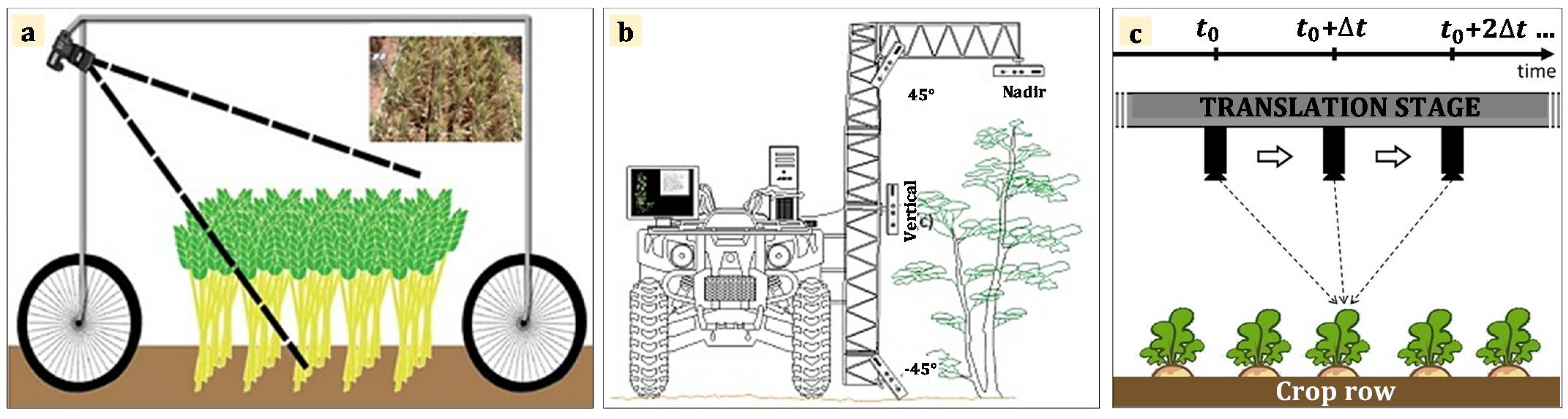
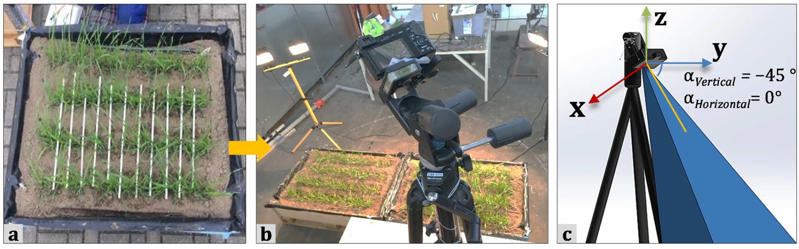
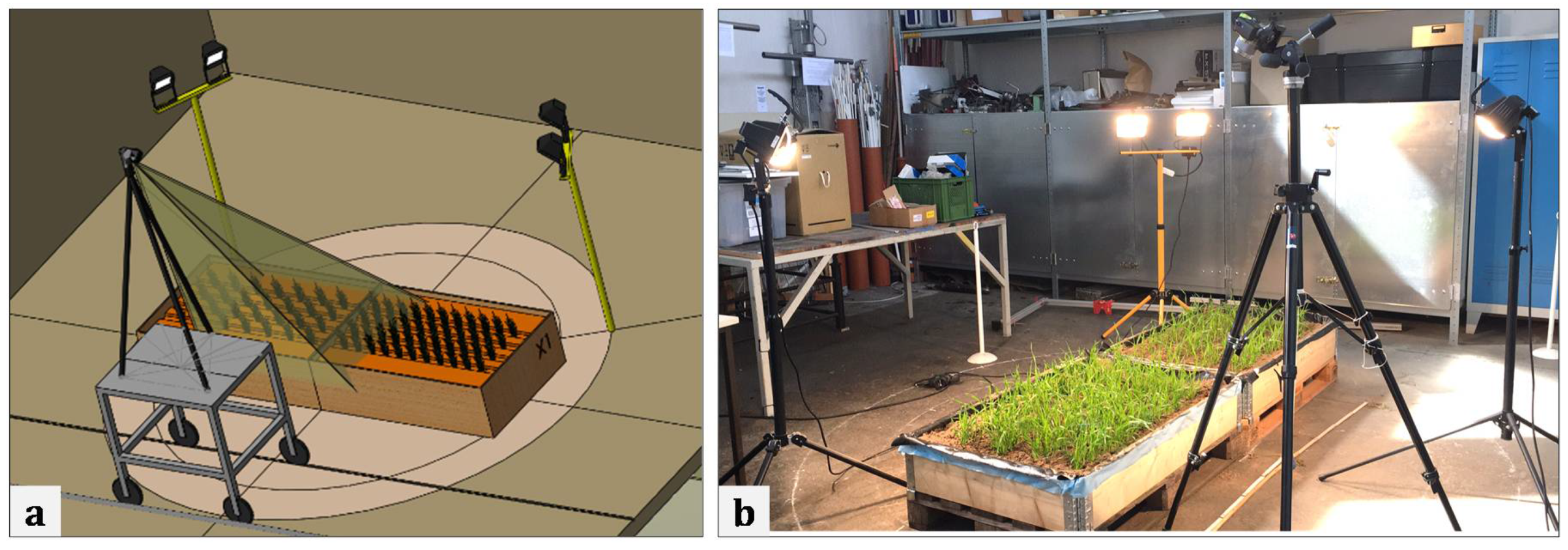
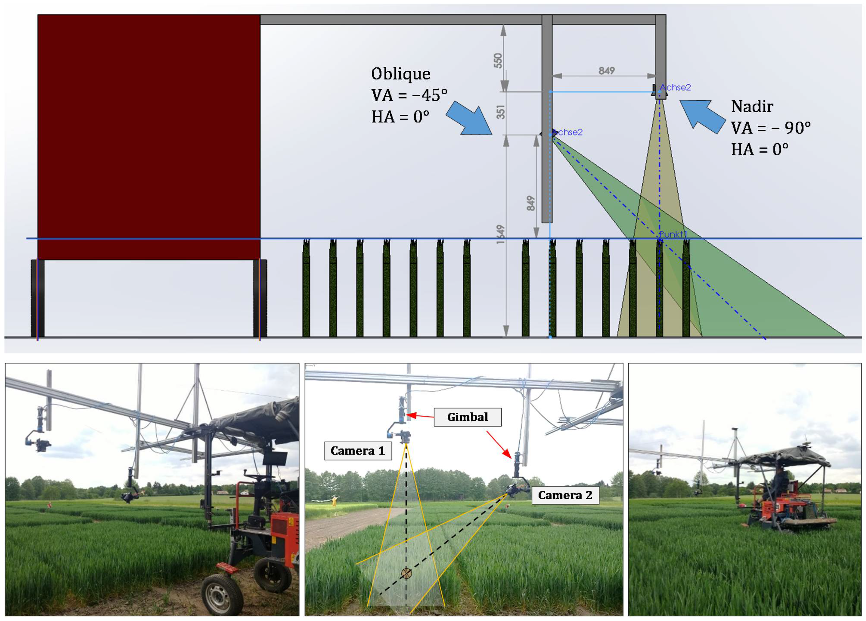
2.1. Experiment Setup and Data Collection

The experiments with different camera viewing angles were conducted inside an indoor laboratory to eliminate external effects at the premises of the Leibniz Institute for Agricultural Engineering and Bioeconomy in Potsdam, Germany (52°26′ N, 13°00′ E). For the experiment, the wheat variety “Kadrilj” has been cultivated in eight pots (100 cm by 17 cm by 14 cm) under controlled conditions in urban garden soil. The wheat plants were seeded in the first four pots with 153 seeds per m² (half density) and in the next four pots with 271 seeds per m² (full density). Figure 2 shows the main steps of the experimental setup and data collection. Each of the four pots with the same planting density was assembled into a larger square pot in order to form an artificial canopy of four rows with a spacing of 17 cm as shown in Figure 2a. The garden soil and the pot edges were entirely covered with sandy, loamy soil from the natural topsoil taken from a crop field.

An overhead view of the experiment site is shown in Figure 2b. Camera viewing angels include (a) the vertical angle (${\alpha }_{Vertical}$, or VA), which is the angle between the vector and xy-plane, (b) the horizontal angle (${\alpha }_{Horizontal}$, or HA), which is the angle between the vector and xz-plane, and (c) a nadir view (vertically, the vector pointing straight downwards) simulating a single camera installed on a low ground vehicle platform. Both ground planes have their origin at the camera position (Figure 2c). A complete horizontal viewing angle was not adopted.

A simulation representation and an actual view of the experimental setup are given in the Figure 3a,b. An adjustable platform with cameras, tripods, and simulated wheat plants were first designed in the SolidWorks software environment (SolidWorks, Waltham, MA, USA) as shown in the Figure 3a to carry out preliminary tests with different camera angles while the platform moved a distance of 10 cm in each iteration. The setup was then built and used to acquire actual wheat canopy imagery from different viewing angles and positions as shown in Figure 3b. The moving platform is a custom-built tool carrier that was made of one steel plate, two horizontal rods, and four vertical aluminum rods to provide maximum stability. A 3-axis adjustable camera tripod enables user-defined camera viewing angles toward the wheat canopy as shown in Figure 3b. Additionally, the Cartesian coordinate system was set in a way that the origin is the focus of a camera, and the vector of viewing angle is the centerline of the field of view. The x-axis and y-axis are horizontal, where the x-axis is perpendicular to the forward direction, and the y-axis is parallel to the forward direction. The z-axis is vertical to the xy-plane and vertically upward.

The camera used for capturing the images was a Sony Alpha 6000 (24 megapixels, sensor size: 23.5 by 15.4 mm, aperture angle: 26.7°, Sony Corporation, Tokyo, Japan) attached with a 50 mm lens (E50 f/1.8). The setup of image acquisition is equivalent to a ground vehicle collecting images in a field—looking at the wheat canopy at different specific viewing angles from one side (oblique view) or from above (nadir view). In total, 3861 images were collected with a 10 cm shooting interval resulting in an 88% overlap for the wheat growth stages BBCH 47 (end of booting) and BBCH 69 (end of flowering). The camera position’s height is adjustable to ensure that the shortest distance from the camera lens center to the middle-top of the canopy is consistent between different viewing angles within each growth stage to obtain a comparable average canopy sampling distance. Detailed information about the image acquisition setup along with the core technical specifications of the camera are listed in

Table 1. Camera acquisition and specification data.

Functional Data	General Data
Vertical angle: −30°, −45°	50 mm lens (E50 f/1.8)
Horizontal angle: 0°, 30°, 45°	24 Megapixel
Nadir view	Aperture angle: 26.7°
Shooting interval: 10 cm in x-axis	Sensor size: 23.5 by 15.4 mm (APS-C)

.

In the field experiment, an equipment carrier vehicle with a custom-built frame for crop scouting (shown in Figure 4) was also used to mount a two-camera system at −45° and nadir angles in order to carry out the reconstruction of 3D point clouds inside the field that were needed for the improvement of crop canopy estimation. The schematic side view of the platform and the actual camera arrangement on the sample pots area are shown in Figure 4. It should be noted that the position of the vertical poles and the height of the gimbal were made adjustable with different canopy heights of the wheat plants.

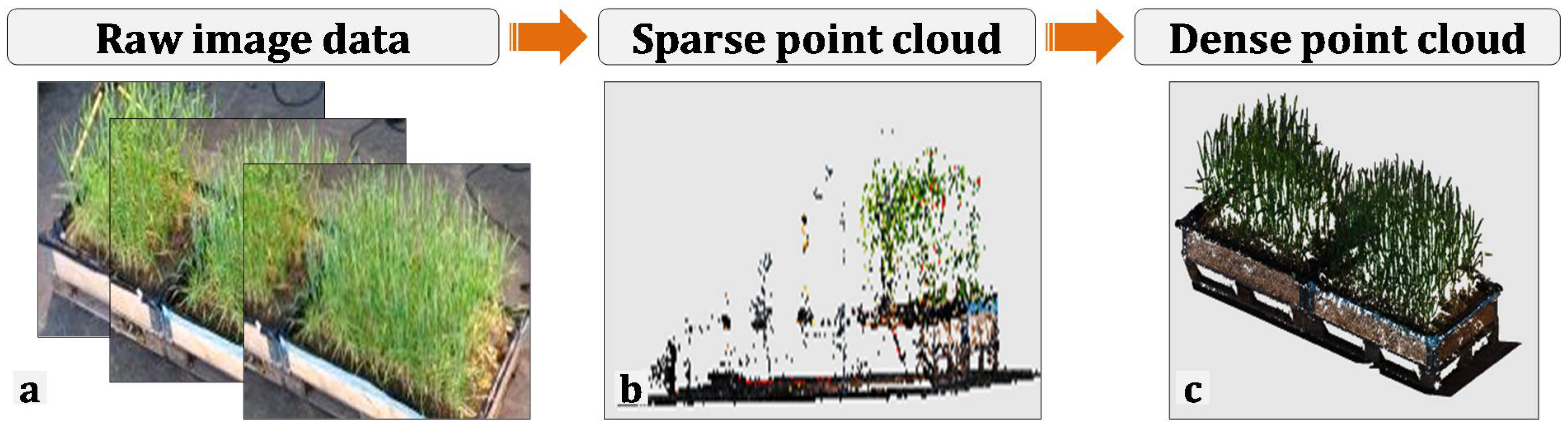
2.2. Generation and Processing of 3D Point Clouds

The 3D sparse point clouds were generated using the SfM approach by means of VisualSFM [46] software, which was available for free, and provided shared-source application codes that include the different SfM photogrammetry steps, i.e., point matching, camera estimation, and bundle adjustment. For the initialization of the camera parameters, VisualSFM [46] used the images’ EXIF data. The detection and description of keypoints were performed with Scale Invariant Feature Transform (SIFT) using the implementation SIFTGPU [60] for fast parallel processing with GPU units. PMVS2, an open-source tool for MVS reconstruction [61], was used for dense 3D reconstruction combined with VisualSFM. The 3D point clouds were generated for each viewing angle separately. 3D point clouds that are generated from multiple viewing angles were used as a reference point cloud. Eight individual point clouds were calculated for each growth stage and saved as PLY files. The 3D point clouds were classified into the wheat canopy, soil background, and experimental square pot. For extracting the experimental square pots, manual clipping was used in the Software CloudCompare. For extracting only the wheat canopy from the soil background, RGB thresholding was used with the settings R < 20, G > 100 and B > 150. The 3D point clouds of wheat canopy structure were generated based on the nadir, multiple-view, and six oblique view image datasets from a set of overlapping, uncalibrated raw images using SfM-MVS methods, and the process was shown in Figure 5.

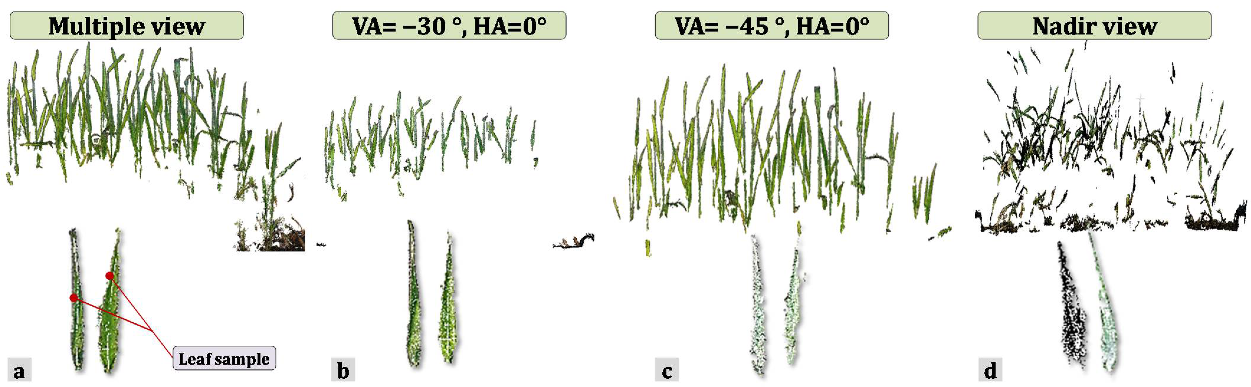
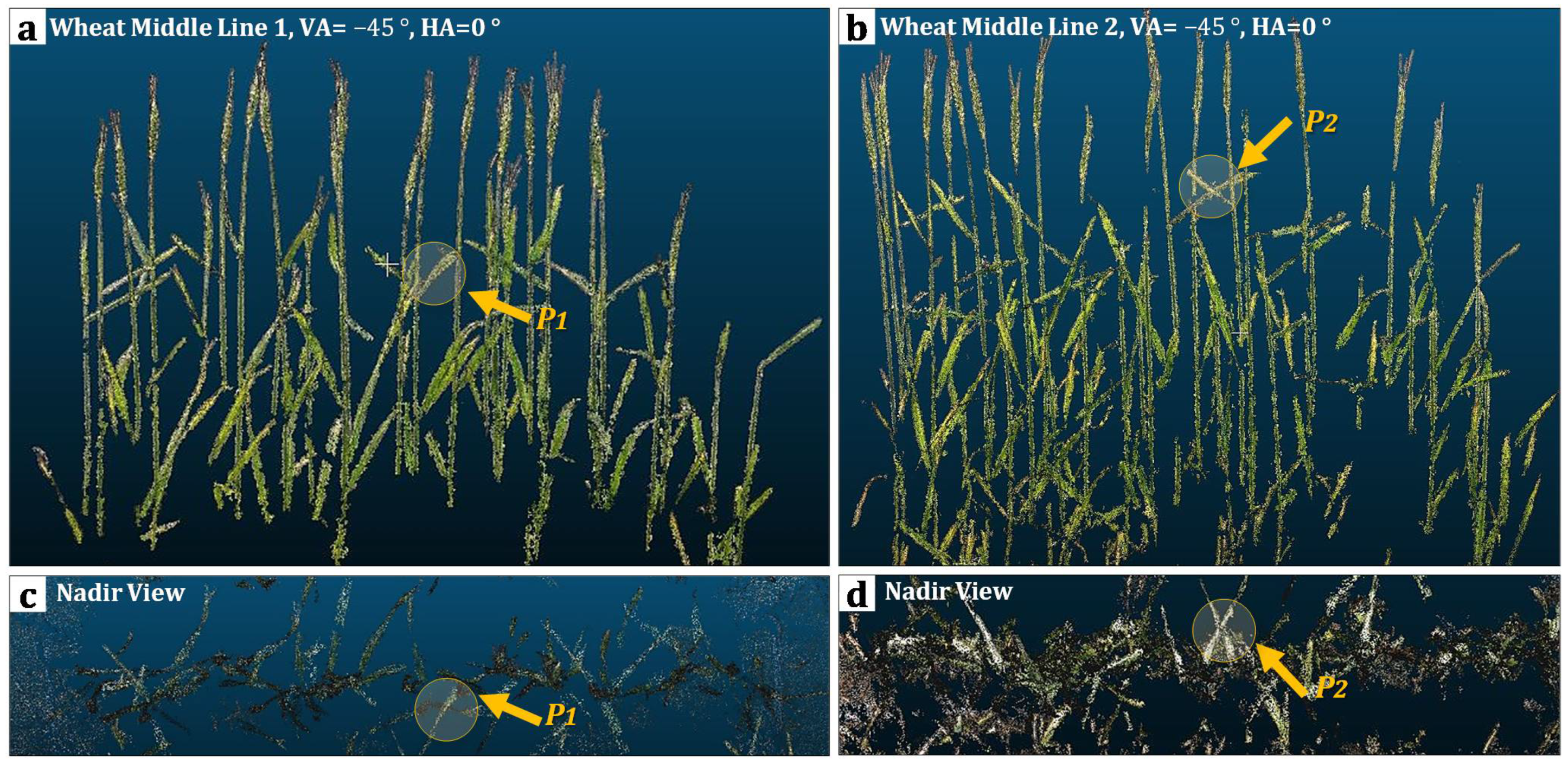
2.3. Validation of the 3D Point Clouds and Optimization of Angle Factors

As reference measurement, plant morphological data was collected from the two middle rows in which the leaf length and leaf width from 10 randomly selected wheat plants were measured. The selected plants were marked by a small pin that was put into the soil in their vicinity. Additionally, their serial numbers of a total of 10 were recorded by numbering the plants from one side of the middle rows. Then, the measuring procedure was conducted by operators. The lengths and widths of the first complete leaf of each plant were manually measured with a ruler directly after image acquisition in its rolled-out position. The length was measured along the midline position of each leaf, and the width was measured at a position where maximum width was obtained.

To extract the leaf width and length from the point clouds, CloudCompare tools were used to measure virtually the leaves in the 3D environment. All virtual leaf measurements were converted to real values by using the scale taken from the exterior length of the experimental square pots. To assess the point clouds quantitatively, the mean absolute percentage error (MAPE), the mean error (ME), and the mean absolute error (MAE) between the converted virtual measurements of leaf length and width (ŷ) and the reference measurements (y) were calculated by:

$$MAPE=\frac{1}{n}{\displaystyle \sum }_{i=1}^n\left|\frac{\widehat{y}-y}{y}\right|*100\%$$

(1)

$$ME=\frac{1}{n}{\displaystyle \sum }_{i=1}^n{\widehat{y}}_i-y_i$$

(2)

$$MAE=\frac{1}{n}{\displaystyle \sum }_{i=1}^n\left|{\widehat{y}}_i-y_i\right|$$

(3)

The error percentages vary between zero, where negative values denote that leaves are represented smaller in the point clouds than in reality, and positive values vice versa. Error percentages were summarized by means of box plots. The size of the box plots represents the number of adequately conducted measurements. In addition, in order to find the optimum camera angle factor in the vertical and horizontal view, the collected leaf length and width data were investigated with Response Surface Methodology (RSM) [62]. The results were then analyzed in the R statistical software (R Development Core Team, 2008) [63], by means of a package called “rsm” that is based on a central composite design [64]. The package fitted a second-degree polynomial with response-surface components. The established RSM then defined VA as the abscissa and horizontal angle (HA) as the ordinate. This contributed to a better visual expression of the relationship between the camera viewing angle combination and the average error. It should be noted that this approach contributed to significant laboratory time saving that would have been required for adjusting all possible angles between 0−30° and 30–45° in order to find the angle that leads to the minimum average error (known as the optimum angle). Figure 6 shows the measurement for validation. In the last trial, destructive method was used for wheat plants to measure leaf parameters (Figure 6a,b). Figure 6c shows the representation of a single row with one wheat density, and it constitutes the density of the wheat canopy.

3. Results and Discussion

3.1. Quality of the 3D Point Clouds over Different Viewing Angles

The 3D point clouds of the wheat canopy from a middle row were selected to represent and compare the quality of the reconstructed canopy structure based on different view image datasets. Figure 7 shows the front view of the point cloud along with two randomly selected examples of leaves representing the camera setup as multiple views (Figure 7a), two single views (Figure 7b: VA = −30°, HA = 0° and Figure 7c: VA = −45°, HA = 0°), and the nadir view (Figure 7d). The wheat canopy has reached the growth stage BBCH47 with the flag leaf sheath opening. From the results on the point clouds, it can be seen that the quality of point cloud for the wheat canopy from that middle row varies in their visibility and completeness depending on which perspective the image dataset was acquired.

Figure 8 shows the 3D point clouds of two wheat rows in the middle of the canopy at growth stage BBCH 69. They were calculated from two viewing angles: front view with vertical angle of −45° and horizontal angle of 0° (Figure 8a,b), as well as nadir view (Figure 8c,d). Points P1 and P2 are leaf samples. Although the point P1 and P2 samples can be identified as reconstructed point clouds of the same leaves, the geometry of the leaf still differs considerably between the top images and the bottom images. The point cloud obtained from a single oblique view can be useful for observing leaves, superior to correctly delineating the wheat leaves from nadir perspective. In addition, the bottom images similarly confirm that more ground information of the canopy can be seen.

The point cloud based on the multi-view images incorporates the broadest view on different parts of the plants, thus through SfM-MVS workflow, it can be observed that the most underlying parts of the canopy, show the most fully reconstructed 3D point cloud of the canopy and acquire the most comprehensive set of information. Because in the case of a multi-view camera system, the canopy is viewed from multiple angles allowing one to gather images of the plants from different perspectives. However, even in this case, some problems occurred in properly delineating the wheat stem in the lower positions. These are due to the front rows obscuring the back ranks in the wheat canopy, which was universal for all viewing angles investigated here except for the nadir view. The quality of the point clouds from the imagery based on a single oblique perspective, in this case, the view with the vertical angles of −30° and −45°, respectively, and a constant horizontal angle of 0°, showed fewer plant structures than the point clouds reconstructed from multi-view images. It was also found that these two angles led to point clouds with different qualities. The point cloud based on the vertical angles of −45° represented the canopy with more plant structures than the one based on a vertical angle of −30°. Zooming in on individual plant leaves in the point clouds, it becomes evident that the point clouds also differ in the density and number of 3D points that constitute the plant structures. The point cloud derived from the nadir images differed even more substantially from the point cloud structure based on the multiple views. Wheat leaves had strongly broken characteristics in the point cloud and were therefore difficult to measure. Additionally, the shape of the plant leaves differed geometrically from the other point clouds. Wheat canopies have mostly an erectophile leaf angle distribution, which means that the leaves are standing upright, pointing with their tips to the sun. In the case of the nadir view, the full body of the plant leaves is only a little exposed towards the camera. In return, this view allows for collecting information from the lower parts of the canopy so that even the canopy ground was visible in the nadir point cloud. This can be used when the target is to measure the canopy height instead of leaf geometries. The fact that the representation of the wheat canopy varied between the point cloud examples showed that the camera viewing angle influences the quality of the point cloud and further the 3D variables of the canopy.

Concerning the field experiment, in the feature pair matching step, various attempts failed to match or correctly match the image feature pairs, thus failing to recover the correct 3D geometric information from the image sequence. The reasons for the failure of the experiment can be attributed to multiple reasons, including (i) the environmental factors in the field experiment site, such as disturbance of wind, ambient light, mechanical vibration, and playing a role of the main obstacles for using this 3D reconstruction method directly in the low-altitude image sequences, (ii) not having enough reoccurrence of the same feature points from wheat, as many feature points of the canopy were lost or inconsistent among adjacent images after feature extraction, and (iii) unavailability of high heterogeneity and lack of fixed references such as soil surface for image regions and inside the field. These reasons ultimately resulted in a lack of stable feature point pairs and also led to the refusal to match or mismatching of feature space outliers by the SfM photogrammetry.

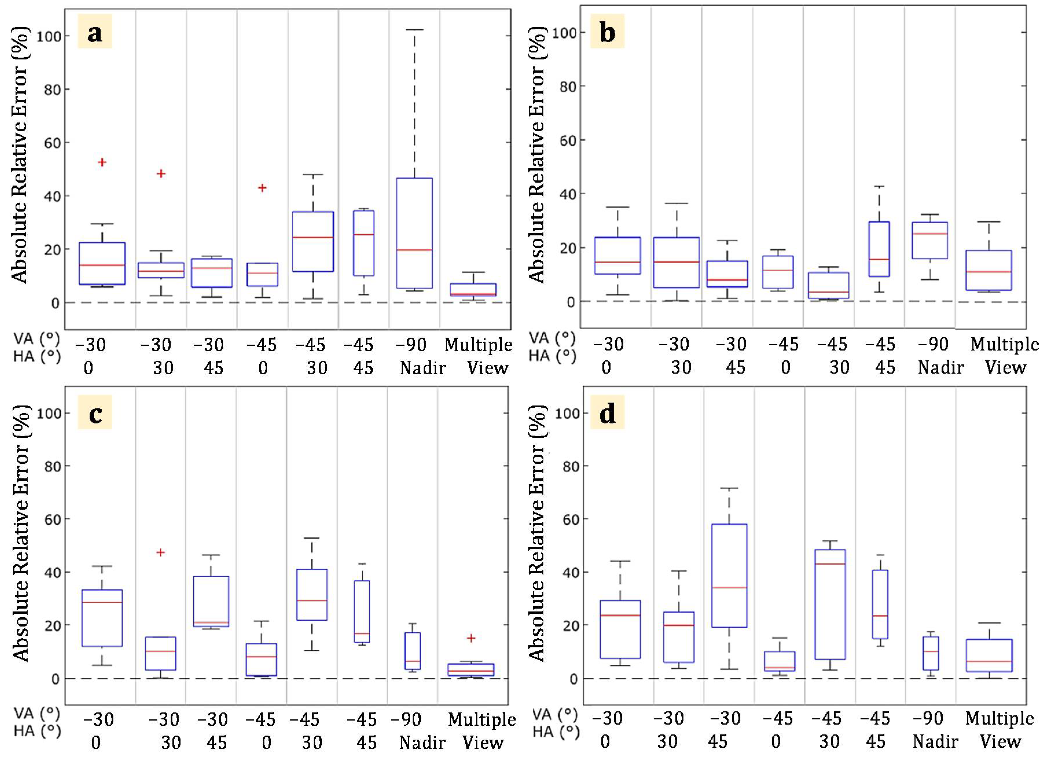
3.2. Quantitative Evaluation and Simulated Influence of Viewing Angle

In

Table 2. Summary of leaf accuracies and missing leaf rate for the reconstructed model.

	Parameter	Error Type	Multiple View	VA −30°			VA −45°			Nadir View
				HA0	HA30	HA45	HA0	HA30	HA45
BBCH47	Length	ME (cm)	−0.24	−2.43	−1.51	−1.14	−0.62	−3.38	−1.81	3.90
		MAE (cm)	0.65	2.70	2.32	1.61	1.19	3.51	3.00	4.20
		MAPE (%)	4.73	18.30	15.02	11.10	8.89	23.62	22.22	32.89
	Width	ME (cm)	0.14	0.15	0.14	0.05	0.12	−0.03	−0.24	−0.04
		MAE (cm)	0.16	0.20	0.18	0.12	0.16	0.07	0.24	0.27
		MAPE (%)	13.38	16.92	15.38	10.00	12.51	5.50	19.37	22.88
	Missing leaf rate	Percentage (%)	10%	10%	10%	20%	40%	20%	60%	30%
BBCH69	Length	ME (cm)	−0.27	3.35	−1.96	3.92	−0.88	3.39	3.04	0.41
		MAE (cm)	0.50	3.35	1.96	3.92	1.28	4.09	3.05	1.24
		MAPE (%)	2.72	21.63	14.37	28.10	8.71	30.72	24.17	9.77
	Width	ME (cm)	0.10	0.20	0.17	0.45	−0.05	0.38	0.33	−0.04
		MAE (cm)	0.10	0.24	0.23	0.45	0.07	0.38	0.33	0.11
		MAPE (%)	8.88	21.15	19.10	38.03	6.14	32.72	27.28	9.44
	Missing leaf rate	Percentage (%)	10%	20%	40%	30%	40%	40%	70%	70%

, the comparison between the estimation from the 3D point clouds and the measurements of the actual leaves are summarized to assess the quality of the different point clouds quantitatively.

The best quality was obtained for the point clouds derived from images that were taken from multiple camera angles. With a missing leaf rate of only 10% for both growth stages, they were the most complete point clouds. Moreover, in terms of accuracy, point clouds using images from multiple angles showed better results. The best measurements were obtained for the later growth stage BBCH 69 with only 0.5 cm difference to the actual leaf length and only 0.1 cm difference to the actual leaf width. Generally, leaf length was measured with a lower MAPE and uncertainty than leaf width.

Regarding the single-angle point clouds excluding the nadir view, they had lower quality than those derived from the multiple-angle view. For leaf length, the mean absolute error ranged between 1.19 cm and 3.51 cm that is 8.89% and 23.69% MAPE for BBCH 47, and between 1.28 cm and 4.09 cm that is 8.71% and 30.72% MAPE for BBCH 69. The missing rate strongly varied from 10% to 70%. Leaf width estimation from a single angle perspective excluding nadir view was slightly more accurate than compared for leaf length estimation but with a large range of MAPE among the different angle views. MAPE ranged from 5.50% to 19.37% with 0.07 cm to 0.24 cm mean absolute error for BBCH 47 and from 6.14% to 38.03% with 0.07 cm to 0.38 cm mean absolute error for BBCH 69. The best camera angle was the same for both growth stages (VA-45, HA0), which leads to a preferred setting of a direct camera view of −45° towards the plant canopy seems to be preferred. This view had the best trade-off balance between accuracy and missing leaf rate. This practice is observed in other published worked (i.e., [65,66]) that mounted the one camera for data acquisition at −45° degree in inclination perpendicular to the row direction (VA-45, HA0) on a moving vehicle to estimate the wheat plant density at early stages using 2D RGB images in all the experimental cases. However, the latter was accounted for having still 40% of the leaves not measurable. The better quality of the point clouds from multiple angles can be explained by the fact that these images reached the highest coverage of the plants. Parts of the canopy that are not depicted in the images can also not be estimated within the SfM pipeline leading to worse quality of the 3D point clouds of plant leaves [67]. SfM point clouds generated from a single angle perspective will suffer to some extent from this problem when modeling plant canopies. The nadir models were mostly different between the two growth stages. For BBCH 47, the mean absolute error for leaf length and width were the least effective with a 4.2 cm difference meaning 32.89% MAPE to the measured leaf length and 0.27 cm difference, meaning 22.88% MAPE to the measured leaf width. Figure 9 shows boxplots of the absolute percentage error of leaf length and leaf width at growth stages of BBCH 47 and BBCH 69, respectively. The boxplots reveal more detailed information at each growth stage for each leaf parameter.

The most significant error exceeded 100%, and reached 102% (Figure 9a). This error comes from the different shapes between the leaf in the modeling and the actual leaf. From the initial image matching to the later MVS, there are possibilities, eventually leading to reconstruction errors. For BBCH 69, MAPE was 9.77%, meaning a 1.24 cm difference to the measured leaf length, and 9.44% meaning 0.11 cm difference to the measured leaf width. However, the missing leaf rate was 70% (Figure 9c,d), which means that only very little valid data was actually obtained from the nadir images, although the results for the very few modeled plant leaves were strikingly accurate, ranking second only after the best model. This reason can be partly explained by the fact that adjacent plants have less mutual effect when in the case of nadir perspective than in the oblique imagery. Díaz (Díaz, 2020), in his research, confirmed the benefit of adding oblique image set to nadir image set by combing UAS nadir and −45° (VA45, HA0) imagery for estimation of the forest canopy.

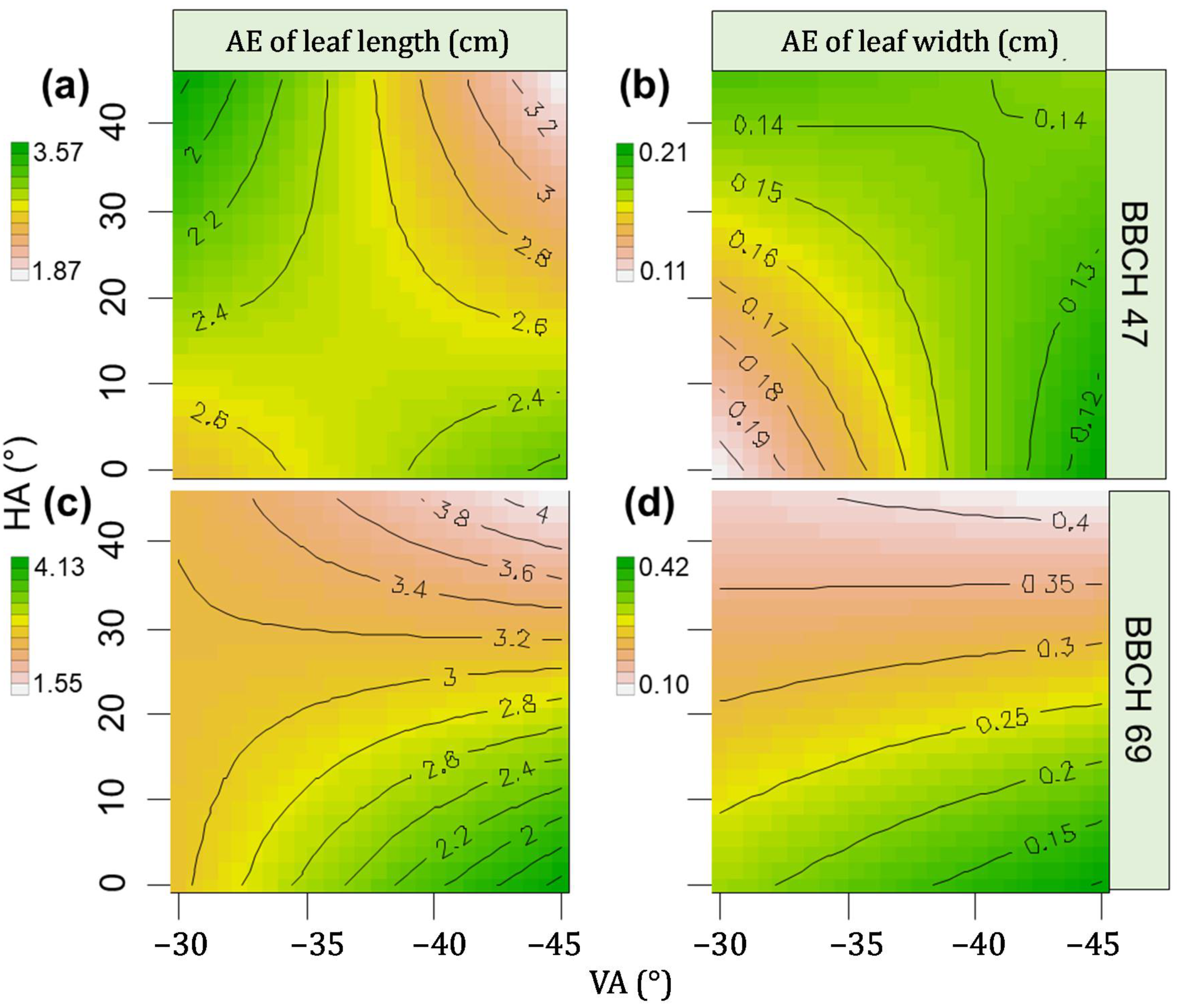
3.3. Visualizaion of the Response Surface Model and Optimum Viewing Angle

The RSM simulation confirmed considerable diversity between all possible viewing angles and resulted in finding the optimum values. It was further verified by response surface methodology that, the angle settings can contribute to improving the evaluation of crop parameters and the optimal oblique angle parameters for two growth cycles were given as vertical angle −45° and horizontal angle 0°. From the results, it can be seen that the vertical angle−30° and horizontal angle 45°, as well as the vertical angle −45° and horizontal angle 0° at the BBCH47 (Figure 10a,b), can yield leaf length and leaf width estimates with small errors. Among them, vertical angle −45°and horizontal angle 0° are slightly better than vertical angle −30° and horizontal angle 45° in estimating blade width. In terms of estimated length, the opposite is true, with slightly better estimates at the latter angle setting. During this growth cycle, the absolute error values varied from 1.87 to 3.57 cm (absolute error in leaf length) and from 0.11 to 0.21 cm (absolute error in leaf width), respectively. Compared to the worst error results, within each parameter, the absolute errors were able to differ by a maximum of 1.7 cm and 0.1 cm. At the BBCH69 (Figure 10c,d), a vertical angle of −45° and a horizontal angle of 0° allowed to obtain estimates of blade length and blade width with small errors. At that growth cycle, the absolute range of values varied from 1.55 to 4.13 cm (absolute error in leaf length), and from 0.10 to 0.42 cm (absolute error in leaf width), respectively. In comparison with the worst error results, the absolute errors were able to differ by a maximum of 2.58 cm and 0.32 cm within each parameter. In summary, vertical angle −45° and horizontal angle 0° were the optimal angle setting results. Based on the simulated interaction effects results, it is also shown that the optimal angle will facilitate the acquisition of canopy parameters from the 3D model.

The impact of viewing angle as shown in this study adds to the discussion in digital agriculture for estimating reliable plant parameters. For example, Andujar et al. [43] evaluated different camera angles for best estimation of plant biomass from poplar seedlings using an RGB-D camera approach and concluded that the best camera angle was dependent on the tree structure, leaf density, and leaf position, so, the growth stage should be taken into account when a correct camera angle is chosen. Similar result was obtained by Nguyen et al. [68] who investigated multi-view reconstruction of eggplants when developing a 3D computer vision-based plant phenotyping technology based on stereovision to estimate number of leaves, leaf area, and plant height. They found that the camera angle was depending on the plant growth. For smaller, younger plants, nadir view achieved best results whereas for larger plants the oblique views provided greater information content in the 3D reconstruction. Oblique view images have also been applied from the UAV platform. Hobart et al. [56] used oblique view imagery for estimating tree heights in an apple orchard to maximize the information content by looking side-views onto the tree-rows. They could successfully calculate 3D point clouds with high correlation with ground-based LiDAR values.

4. Conclusions

This study showed that the photogrammetric SfM-MVS method generated high quality 3D point clouds that were capable to accurately estimate leaf length and width of wheat plants when images were used from cameras viewing from different directions towards the canopy. In the case of a single camera view, the quality of the 3D point cloud was generally lower, and the degree of quality was highly dependent on which viewing angle was used towards the canopy. We proposed a setup for the mono−camera system that a direct viewing angle of −45° would be the most efficient viewing angle for measuring leaf length and width. It can be concluded that using the viewing angle −45° for a single camera scenario to detect leaf canopy variables in the crop is a promising way in precision agricultural applications to estimate crop status for site-specific crop management while considering crop protection, fertilization, and plant disease. The use of only one camera for 3D sensing showed advantages and proved that it enable easy duplication of the system, increase the degree of freedom (no fixed angle adjustment and distance to the plants) and reduce costs. The mono-camera system features an easily accessible and simple structure with lesser technical efforts concerning the hardware than the binocular-camera system. This paper also looked at the results from the perspective of exploiting oblique imagery solutions of retrieving 3D plant information, especially for field phenotyping with SfM photogrammetry. Based on the results of this research, the use of oblique imagery can improve the estimation of plant parameters and should be more considered when camera setups are conceptualized for phenotyping or precision agriculture. Further research should examine this optimum setup of a mono-camera system to collect more information on angles to improve robustness via an indoor experiment. In addition, new field experiments will consider avoiding the above interferences and consider adding information such as ground-truthing, references to ensure and improve the reconstruction of the field 3D crop canopy inside the field from low-altitude imagery.

References

1. Comba, L.; Biglia, A.; Aimonino, D.R.; Tortia, C.; Mania, E.; Guidoni, S.; Gay, P. Leaf Area Index evaluation in vineyards using 3D point clouds from UAV imagery. Precis. Agric. 2020, 21, 881–896. [Google Scholar] [CrossRef] [Green Version]
2. Garcerá, C.; Doruchowski, G.; Chueca, P. Harmonization of plant protection products dose expression and dose adjustment for high growing 3D crops: A review. Crop Prot. 2021, 140, 105417. [Google Scholar] [CrossRef]
3. Jiménez-Brenes, F.M.; López-Granados, F.; de Castro, A.I.; Torres-Sánchez, J.; Serrano, N.; Peña, J.M. Quantifying pruning impacts on olive tree architecture and annual canopy growth by using UAV-based 3D modelling. Plant Methods 2017, 13, 1–15. [Google Scholar] [CrossRef] [PubMed] [Green Version]
4. Montgomery, K.; Henry, J.B.; Vann, M.C.; Whipker, B.E.; Huseth, A.S.; Mitasova, H. Measures of canopy structure from low-cost UAS for monitoring crop nutrient status. Drones 2020, 4, 36. [Google Scholar] [CrossRef]
5. Gené-Mola, J.; Gregorio, E.; Cheein, F.A.; Guevara, J.; Llorens, J.; Sanz-Cortiella, R.; Escolà, A.; Rosell-Polo, J.R. Fruit detection, yield prediction and canopy geometric characterization using LiDAR with forced air flow. Comput. Electron. Agric. 2020, 168, 105121. [Google Scholar] [CrossRef]
6. Ramin Shamshiri, R.; Weltzien, C.; Hameed, I.A.; Yule, I.J.; Grift, T.E.; Balasundram, S.K.; Pitonakova, L.; Ahmad, D.; Chowdhary, G. Research and development in agricultural robotics: A perspective of digital farming. Int. J. Agric. Biol. Eng. 2018, 11, 1–14. [Google Scholar] [CrossRef]
7. Ramin Shamshiri, R.; Hameed, I.A.; Pitonakova, L.; Weltzien, C.; Balasundram, S.K.; Yule, I.J.; Grift, T.E.; Chowdhary, G. Simulation software and virtual environments for acceleration of agricultural robotics: Features highlights and performance comparison. Int. J. Agric. Biol. Eng. 2018, 11, 15–31. [Google Scholar] [CrossRef]
8. Jurado, J.M.; Ortega, L.; Cubillas, J.J.; Feito, F.R. Multispectral mapping on 3D models and multi-temporal monitoring for individual characterization of olive trees. Remote Sens. 2020, 12, 1106. [Google Scholar] [CrossRef] [Green Version]
9. Babar, M.A.; Reynolds, M.P.; van Ginkel, M.; Klatt, A.R.; Raun, W.R.; Stone, M.L. Spectral reflectance to estimate genetic variation for in-season biomass, leaf chlorophyll, and canopy temperature in wheat. Crop Sci. 2006, 46, 1046–1057. [Google Scholar] [CrossRef]
10. Li, F.; Gnyp, M.L.; Jia, L.; Miao, Y.; Yu, Z.; Koppe, W.; Bareth, G.; Chen, X.; Zhang, F. Estimating N status of winter wheat using a handheld spectrometer in the North China Plain. Field Crop. Res. 2008, 106, 77–85. [Google Scholar] [CrossRef]
11. Hosoi, F.; Omasa, K. Estimating vertical plant area density profile and growth parameters of a wheat canopy at different growth stages using three-dimensional portable lidar imaging. ISPRS J. Photogramm. Remote Sens. 2009, 64, 151–158. [Google Scholar] [CrossRef]
12. Whan, B.R.; Carlton, G.P.; Anderson, W.K. Potential for increasing early vigour and total biomass in spring wheat. I. Identification of genetic improvements. Aust. J. Agric. Res. 1991, 42, 347–361. [Google Scholar] [CrossRef]
13. Tremblay, N.; Wang, Z.; Ma, B.-L.; Belec, C.; Vigneault, P. A Comparison of crop data measured by two commercial sensors for variable-rate nitrogen application. Precis. Agric. 2009, 10, 145–161. [Google Scholar] [CrossRef]
14. Erdle, K.; Mistele, B.; Schmidhalter, U. Comparison of active and passive spectral sensors in discriminating biomass parameters and nitrogen status in wheat cultivars. F. Crop. Res. 2011, 124, 74–84. [Google Scholar] [CrossRef]
15. Gianelle, D.; Guastella, F. Nadir and off-nadir hyperspectral field data: Strengths and limitations in estimating grassland biophysical characteristics. Int. J. Remote Sens. 2007, 28, 1547–1560. [Google Scholar] [CrossRef]
16. Houborg, R.; Anderson, M.; Daughtry, C. Utility of an image-based canopy reflectance modeling tool for remote estimation of LAI and leaf chlorophyll content at the field scale. Remote Sens. Environ. 2009, 113, 259–274. [Google Scholar] [CrossRef]
17. Bates, J.S.; Montzka, C.; Schmidt, M.; Jonard, F. Estimating canopy density parameters time-series for winter wheat using UAS Mounted LiDAR. Remote Sens. 2021, 13, 710. [Google Scholar] [CrossRef]
18. Zhou, Z.; Majeed, Y.; Naranjo, G.D.; Gambacorta, E.M.T. Assessment for crop water stress with infrared thermal imagery in precision agriculture: A review and future prospects for deep learning applications. Comput. Electron. Agric. 2021, 182, 106019. [Google Scholar] [CrossRef]
19. Shamshiri, R.R.; Hameed, I.A.; Balasundram, S.K.; Ahmad, D.; Weltzien, C.; Yamin, M. Fundamental research on unmanned aerial vehicles to support precision agriculture in oil palm plantations. In Agricultural Robots; Zhou, J., Zhang, B., Eds.; IntechOpen: Rijeka, Croatia, 2019. [Google Scholar]
20. Zhou, Z.; Morel, J.; Parsons, D.; Kucheryavskiy, S.V.; Gustavsson, A.M. Estimation of yield and quality of legume and grass mixtures using partial least squares and support vector machine analysis of spectral data. Comput. Electron. Agric. 2019, 162, 246–253. [Google Scholar] [CrossRef]
21. Perroy, R.L.; Sullivan, T.T.; Stephenson, N. Assessing the impacts of canopy openness and flight parameters on detecting a sub-canopy tropical invasive plant using a small unmanned aerial system. ISPRS J. Photogramm. Remote Sens. 2017, 125, 174–183. [Google Scholar] [CrossRef]
22. Du, M.; Noguchi, N. Monitoring of wheat growth status and mapping of wheat yield’s within-field spatial variations using color images acquired from UAV-camera System. Remote Sens. 2017, 9, 289. [Google Scholar] [CrossRef] [Green Version]
23. Cook, S.E.; Bramley, R.G.V. Precision agriculture—opportunities, benefits and pitfalls of site-specific crop management in Australia. Aust. J. Exp. Agric. 1998, 38, 753–763. [Google Scholar] [CrossRef]
24. Banu, S. Precision agriculture: Tomorrow’s technology for today’s farmer. J. Food Process. Technol. 2015, 6, 1–6. [Google Scholar]
25. Whetton, R.L.; Waine, T.W.; Mouazen, A.M. Hyperspectral measurements of yellow rust and fusarium head blight in cereal crops: Part 2: On-line field measurement. Biosyst. Eng. 2018, 167, 144–158. [Google Scholar] [CrossRef] [Green Version]
26. Baresel, J.P.; Rischbeck, P.; Hu, Y.; Kipp, S.; Hu, Y.; Barmeier, G.; Mistele, B.; Schmidhalter, U. Use of a digital camera as alternative method for non-destructive detection of the leaf chlorophyll content and the nitrogen nutrition status in wheat. Comput. Electron. Agric. 2017, 140, 25–33. [Google Scholar] [CrossRef]
27. Webber, H.; Martre, P.; Asseng, S.; Kimball, B.; White, J.; Ottman, M.; Wall, G.W.; Sanctis, G.D.; Doltra, J.; Grant, R.; et al. Canopy Temperature for simulation of heat stress in irrigated wheat in a semi-arid environment: A multi-model comparison. Field Crop. Res. 2017, 202, 21–35. [Google Scholar] [CrossRef]
28. Zhao, C.; Li, H.; Li, P.; Yang, G.; Gu, X.; Lan, Y. Effect of vertical distribution of crop structure and biochemical parameters of winter wheat on canopy reflectance characteristics and spectral indices. IEEE Trans. Geosci. Remote Sens. 2017, 55, 236–247. [Google Scholar] [CrossRef]
29. Adamchuk, V.; Ji, W.; Rossel, R.V.; Gebbers, R.; Tremblay, N. Proximal soil and plant sensing. In Precision Agriculture Basics; John Wiley & Sons, Ltd.: Hoboken, NJ, USA, 2018; pp. 119–140. ISBN 978-0-89118-367-9. [Google Scholar]
30. Pallottino, F.; Antonucci, F.; Costa, C.; Bisaglia, C.; Figorilli, S.; Menesatti, P. Optoelectronic proximal sensing vehicle-mounted technologies in precision agriculture: A review. Comput. Electron. Agric. 2019, 162, 859–873. [Google Scholar] [CrossRef]
31. Mahlein, A.-K. Plant disease detection by imaging sensors—Parallels and specific demands for precision agriculture and plant phenotyping. Plant Dis. 2015, 100, 241–251. [Google Scholar] [CrossRef] [Green Version]
32. Pallottino, F.; Menesatti, P.; Figorilli, S.; Antonucci, F.; Tomasone, R.; Colantoni, A.; Costa, C. Machine vision retrofit system for mechanical weed control in precision agriculture applications. Sustainability 2018, 10, 2209. [Google Scholar] [CrossRef] [Green Version]
33. Vergara-Díaz, O.; Zaman-Allah, M.A.; Masuka, B.; Hornero, A.; Zarco-Tejada, P.; Prasanna, B.M.; Cairns, J.E.; Araus, J.L. A Novel remote sensing approach for prediction of maize yield under different conditions of nitrogen fertilization. Front. Plant Sci. 2016, 7, 1–13. [Google Scholar] [CrossRef] [PubMed] [Green Version]
34. Walter, J.; Edwards, J.; McDonald, G.; Kuchel, H. Photogrammetry for the estimation of wheat biomass and harvest index. F. Crop. Res. 2018, 216, 165–174. [Google Scholar] [CrossRef]
35. Esau, T.; Zaman, Q.; Groulx, D.; Farooque, A.; Schumann, A.; Chang, Y. Machine vision smart sprayer for spot-application of agrochemical in wild blueberry fields. Precis. Agric. 2018, 19, 770–788. [Google Scholar] [CrossRef]
36. Liu, K.; Xu, H.; Liu, G.; Guan, P.; Zhou, X.; Peng, H.; Yao, Y.; Ni, Z.; Sun, Q.; Du, J. QTL Mapping of flag leaf-related traits in wheat (Triticum aestivum L.). Theor. Appl. Genet. 2018, 131, 839–849. [Google Scholar] [CrossRef] [Green Version]
37. Palaniswamy, K.M.; Gomez, K.A. Length-width method for estimating leaf area of rice. Agron. J. 1974, 66, 430–433. [Google Scholar] [CrossRef]
38. Hammer, G.L.; Carberry, P.S.; Muchow, R.C. Modelling genotypic and environmental control of leaf area dynamics in grain sorghum. I. whole plant level. F. Crop. Res. 1993, 33, 293–310. [Google Scholar] [CrossRef]
39. Bos, H. Growth of individual leaves of spring wheat (Triticum aestivum L.) as influenced by temperature and light intensity. Ann. Bot. 1998, 81, 141–149. [Google Scholar] [CrossRef] [Green Version]
40. Cotter, M.; Asch, F.; Hilger, T.; Rajaona, A.; Schappert, A.; Stuerz, S.; Yang, X. Measuring leaf area index in rubber plantations—A challenge. Ecol. Indic. 2017, 82, 357–366. [Google Scholar] [CrossRef]
41. Guo, D.; Sun, Y.-Z. Estimation of leaf area of stem lettuce (Lactuca sativa Var angustana) from linear measurements. Indian J. Agric. Sci. 2001, 71, 483–486. [Google Scholar]
42. Hasan, M.M.; Chopin, H.L.; Miklavcic, S.J. Detection and analysis of wheat spikes using Convolutional Neural Networks. Plant Methods 2018, 14, 1–13. [Google Scholar] [CrossRef] [Green Version]
43. Andújar, D.; Fernández-Quintanilla, C.; Dorado, J. Matching the best viewing angle in depth cameras for biomass estimation based on poplar seedling geometry. Sensors 2015, 15, 12999–13011. [Google Scholar] [CrossRef] [Green Version]
44. Jay, S.; Rabatel, G.; Hadoux, X.; Moura, D.; Gorretta, N. In-field crop row phenotyping from 3D modeling performed using structure from motion. Comput. Electron. Agric. 2015, 110, 70–77. [Google Scholar] [CrossRef] [Green Version]
45. Snavely, N.; Seitz, S.M.; Szeliski, R. Modeling the world from internet photo collections. Int. J. Comput. Vis. 2008, 80, 189–210. [Google Scholar] [CrossRef] [Green Version]
46. Wu, C. VisualSFM: A Visual Structure from Motion System. 2011. Available online: http://ccwu.me/vsfm/ (accessed on 20 May 2021).
47. Seitz, S.M.; Curless, B.; Diebel, J.; Scharstein, D.; Szeliski, R. A comparison and evaluation of multi-view stereo reconstruction algorithms. In Proceedings of the 2006 IEEE Computer Society Conference on Computer Vision and Pattern Recognition (CVPR’06), New York, NY, USA, 17–22 June 2006; Volume 1, pp. 519–528. [Google Scholar]
48. Jimenez-Berni, J.A.; Deery, D.M.; Rozas-Larraondo, P.; Condon, A.G.; Rebetzke, G.J.; James, R.A.; Bovill, W.D.; Furbank, R.T.; Sirault, X.R.R. High Throughput determination of plant height, ground cover, and above-ground biomass in wheat with LiDAR. Front. Plant Sci. 2018, 9, 237. [Google Scholar] [CrossRef] [Green Version]
49. Le, T.D.Q.; Alvarado, C.; Girousse, C.; Legland, D.; Chateigner-Boutin, A.-L. Use of X-ray micro computed tomography imaging to analyze the morphology of wheat grain through its development. Plant Methods 2019, 15, 84. [Google Scholar] [CrossRef] [Green Version]
50. Dellaert, F.; Seitz, F.M.; Thorpe, C.E.; Thrun, S. Structure from motion without correspondence. In Proceedings of the IEEE Conference on Computer Vision and Pattern Recognition, CVPR 2000 (Cat. No.PR00662), Hilton Head, SC, USA, 13–15 June 2000; Volume 2, pp. 557–564. [Google Scholar]
51. Dandrifosse, S.; Bouvry, A.; Leemans, V.; Dumont, B.; Mercatoris, B. Imaging wheat canopy through stereo vision: Overcoming the challenges of the laboratory to field transition for morphological features extraction. Front Plant Sci. 2020, 11, 96. [Google Scholar] [CrossRef] [Green Version]
52. Cai, J.; Kumar, P.; Chopin, J.; Miklavcic, S.J. Land-based crop phenotyping by image analysis: Accurate estimation of canopy height distributions using stereo images. PLoS ONE 2018, 13, e0196671. [Google Scholar] [CrossRef] [PubMed]
53. Mueller-Sim, T.; Jenkins, M.; Abel, J.; Kantor, G. The Robotanist: A ground-based agricultural robot for high-throughput crop phenotyping. In Proceedings of the 2017 IEEE International Conference on Robotics and Automation (ICRA), Singapore, 29 May–3 June 2017; pp. 3634–3639. [Google Scholar]
54. Kicherer, A.; Herzog, K.; Bendel, N.; Klück, H.-C.; Backhaus, A.; Wieland, M.; Rose, J.; Klingbeil, L.; Läbe, T.; Hohl, C.; et al. Phenoliner: A new field phenotyping platform for grapevine research. Sensors 2017, 17, 1625. [Google Scholar] [CrossRef]
55. Salas Fernandez, M.G.; Bao, Y.; Tang, L.; Schnable, P.S. A High-throughput, field-based phenotyping technology for tall biomass crops. Plant Physiol. 2017, 174, 2008–2022. [Google Scholar] [CrossRef] [PubMed] [Green Version]
56. Hobart, M.; Pflanz, M.; Weltzien, C.; Schirrmann, M. Growth height determination of tree walls for precise monitoring in apple fruit production using UAV photogrammetry. Remote Sens. 2020, 12, 1656. [Google Scholar] [CrossRef]
57. Cheng, M.-L.; Matsuoka, M. Extracting three-dimensional (3D) spatial information from sequential oblique unmanned aerial system (UAS) imagery for digital surface modeling. Int. J. Remote Sens. 2021, 42, 1643–1663. [Google Scholar] [CrossRef]
58. Nesbit, P.R.; Hugenholtz, C.H. Enhancing UAV-SfM 3D model accuracy in high-relief landscapes by incorporating oblique images. Remote Sens. 2019, 11, 239. [Google Scholar] [CrossRef] [Green Version]
59. Che, Y.; Wang, Q.; Xie, Z.; Zhou, L.; Li, S.; Hui, F.; Wang, X.; Li, B.; Ma, Y. Estimation of maize plant height and leaf area index dynamics using an unmanned aerial vehicle with oblique and nadir photography. Ann. Bot. 2020, 126, 765–773. [Google Scholar] [CrossRef]
60. Wu, C. A GPU Implementation of Scale Invariant Feature Transform (SIFT). 2007. Available online: http//www.cs.unc.edu/~ccwu/siftgpu/ (accessed on 20 May 2021).
61. Gonzalez-Aguilera, D.; López-Fernández, L.; Rodriguez-Gonzalvez, P.; Hernandez-Lopez, D.; Guerrero, D.; Remondino, F.; Menna, F.; Nocerino, E.; Toschi, I.; Ballabeni, A.; et al. GRAPHOS—Open-source software for photogrammetric applications. Photogram. Rec. 2018, 33, 11–29. [Google Scholar] [CrossRef] [Green Version]
62. Khuri, A.I.; Mukhopadhyay, S. Response surface methodology. WIREs Comp. Stat. 2010, 2, 128–149. [Google Scholar] [CrossRef]
63. Knezevic, S.Z.; Streibig, J.C.; Ritz, C. Utilizing R software package for dose-response studies: The concept and data analysis. Weed Technol. 2007, 21, 840–848. [Google Scholar] [CrossRef]
64. Lenth, R.V. Response-surface methods in R, using rsm. J. Stat. Softw. 2020, 32, 1–17. [Google Scholar]
65. Su, W.; Zhang, M.; Bian, D.; Liu, Z.; Huang, J.; Wang, W.; Wu, J.; Guo, H. Phenotyping of corn plants using unmanned aerial vehicle (UAV) images. Remote Sens. 2019, 11, 2021. [Google Scholar] [CrossRef] [Green Version]
66. Liu, S.; Baret, F.; Andrieu, B.; Burger, P.; Hemmerlé, M. Estimation of wheat plant density at early stages using high resolution imagery. Front. Plant Sci. 2017, 8, 739. [Google Scholar] [CrossRef] [Green Version]
67. Bianco, S.; Ciocca, G.; Marelli, D. Evaluating the performance of structure from motion pipelines. J. Imaging 2018, 4, 98. [Google Scholar] [CrossRef] [Green Version]
68. Nguyen, T.T.; Slaughter, D.C.; Townsley, B.T.; Carriedo, L.; Maloof, J.N.; Sinha, N. In-Field Plant Phenotyping Using Multi-View Reconstruction: An Investigation in Eggplant, Proceedings of the 13th International Conference on Precision Agriculture, St. Louis, MI, USA, 31 July–4 August 2016; International Society of Precision Agriculture: Monticello, IL, USA, 2016. [Google Scholar]
Figure 1. Example of research works for estimation of plant density from low-altitude imagery and different viewing angle showing (a) detection and analysis of wheat spikes from oblique digital images using CNN [42], (b) biomass estimation using Kinect sensors from different viewing angles in order to match the best viewing angle based on poplar seedling geometry [43], and (c) in-field crop row phenotyping estimation from 3D modeling derived by SfM from top-view RGB images [44].
Agriculture 11 00563 g001
Figure 2. Demonstration of the main steps involved in the experimental for image acquisition with the mono camera system from different viewing angles and positions, showing (a) wheat plants seeded in the square pot, (b) overview of the experiment site, and (c) variable shooting adjustment of the mobile platform.
Agriculture 11 00563 g002
Figure 3. Laboratory experiment setup showing (a) the preliminary simulation tests, and (b) the actual laboratory experiments with wheat plants in the early growth stage. The platform moves a distance of 10 cm in each iteration.
Agriculture 11 00563 g003
Figure 4. Field experiment setup showing schematic side view of the platform and the position of the vertical poles and the height of the gimbal platform (top image), and the actual camera arrangement on the sample plot area (bottom images).
Agriculture 11 00563 g004
Figure 5. Generation of a 3D dense point cloud showing (a) a set of overlapping, uncalibrated raw images captured by digital camera, (b) reconstructed images to a 3D sparse point cloud using SfM, and (c) recovered result using MVS to a dense point cloud.
Agriculture 11 00563 g005
Figure 6. Measurement for validation including (a) leaf length and width measurement in the last trial, (b) leaf parameters estimation in the last trial (destructive method), and (c) representation of a single row with different wheat density.
Agriculture 11 00563 g006
Figure 7. Demonstration of the front view of the BBCH 47, representing camera setting of (a) multiple view, (b) VA = −30°, HA = 0°, (c) VA = −45°, HA = 0°, and (d) nadir view. Upper images are generated 3D models. Lower images are two randomly selected leaf samples from multi-view images and single view images.
Agriculture 11 00563 g007
Figure 8. Demonstration of the 3D point clouds of the two samples of wheat leaves in the middle row of BBCH 69, showing front view resulted from the vertical angle of −45° and the horizontal angle of 0° (a,b), and the results of the camera setting in nadir view (c,d). Points P1 and P2 are samples.
Agriculture 11 00563 g008
Figure 9. Demonstration of the absolute percentage error of (a) leaf length and (b) leaf width (a) at growth stage BBCH 47, and (c) leaf length, 414, and (d) leaf width at growth stage BBCH 69. It should be noted that the width of the boxplot represents the number of reconstructed and measurable samples in each growth stage.
Agriculture 11 00563 g009
Figure 10. Response surface contour plots shows the two- factor interaction of vertical angle (VA, °) and horizontal angle (HA, °) on the absolute error (cm) of the parameters (a) length and (b) width at the BBCH 47 and (c) length and (d) width at the BBCH 69.
Agriculture 11 00563 g010