Article

The Role of Engineering Thermodynamics in Explaining the Inverse Correlation between Surface Temperature and Supplied Nitrogen Rate in Corn Plants: A Greenhouse Case Study

1
Department of Mechanical and Mechatronics Engineering, University of Waterloo, Waterloo, ON N2L 3G1, Canada
2
Plant Agricultural Department, University of Guelph, Guelph, ON N1G 2W1, Canada
*
Author to whom correspondence should be addressed.
Agriculture 2021, 11(2), 101; https://doi.org/10.3390/agriculture11020101
Submission received: 11 December 2020 / Revised: 21 January 2021 / Accepted: 22 January 2021 / Published: 26 January 2021

Abstract

:
Nitrogen stress plays a critical role in corn yield reduction. Thermal remote sensing has many applications: as an assessment tool for urban heat island, as an ecological indicator of ecosystem development, and as a water-stress-detection tool. In this study, it was hypothesized that corn crops supplied with optimum or high rates of nitrogen would have lower surface temperatures compared to corn grown under nitrogen-stressed conditions. Two experiments were conducted in the greenhouse at the University of Guelph, Canada, from the period between 2015 and 2016, involving three rates of nitrogen (high, medium, and low rates) supplied to corn plants after seed emergence. Leaf and whorl temperatures were collected by using a high-resolution thermal camera, an infrared handheld point measurements gun, and a type T thermocouple, respectively. An approximate difference of 2 °C was observed in temperatures between plants receiving high and low rates of nitrogen. These results supported the hypothesis that nitrogen-stressed plants have higher temperatures compared to less stressed plants, at a 0.05 significance level. This study investigated the application of the exergy destruction principle through thermal remote sensing, to detect crop stress at early growth stages under greenhouse conditions, to increase the production and reduce the harmful environmental impact.

1. Introduction

Corn is one of the most important food crops and sources for biofuels grown worldwide [1,2,3,4]. An adequate supply of nitrogen is essential for successful corn production [5,6]. The occurrence of nitrogen stress results in significant changes in plant growth and development [7,8,9]. As corn develops, the amount of nitrogen required will vary with corresponding growth stage [10]. The ability to apply variable rates of nitrogen at the right growth stage is now possible because of advancements in precision agriculture [11,12]. Accurately applying nitrogen at the right time and location is very important in increasing the crop production while decreasing the input costs (e.g., herbicides, pesticides, and nutrients) and reducing the environmental losses, which include the depletion of soil nutrients and the contamination of drinking water.
Different methods are available to detect nitrogen stress, including optical, transmittance, and chlorophyll fluorescence [13,14]. Most of these methods have limitations, including the dependence on chlorophyll concentrations [15,16], high sensitivity to variation in sunlight and soil conditions, lack of sensitivity for stress detection at early growth stages, and size limitations [13]. Alternatively, thermal remote sensing has been used to detect crop water stress, which is based on the assumption that well-irrigated plants transpire and cool leaf surface temperature below the surrounding air temperature [17,18,19]. Transpiration is one of the mechanisms of energy dissipation in crops that also includes convection, conduction, and heat radiation [20,21,22].
The flow of energy has both magnitude and quality. The quality of energy, called exergy, is defined as the maximum useful work for a system moving from a given state to a state of equilibrium with its surroundings [23,24]. Exergy is not conserved; unlike energy, it can be destroyed. Exergy is used in many engineering applications as a decision-making or optimization tool, for instance, in power plant design and operation specifications [25]. In addition, exergy has been used in life cycle assessment [26,27], in resource accounting [28,29,30], and as an ecological indicator of ecosystem development, complexity, and integrity [31,32,33,34,35,36,37].
The exergy destruction principle states that ecosystem development is associated with maximizing the amount of work available for the purpose of structural organization, function, and survival [32,33,38]. Ecosystems are complex, non-equilibrium thermodynamic systems that are open to energy and mass flows. Ecosystems maintain their organization and structure through continuous energy dissipation [39,40,41,42]. As ecosystems develop and mature, they will increase their total energy dissipation and the use of available exergy; thus, they will develop more complex structures with greater diversity [38,43]. The organization and complexity of an ecosystem increases with the increase in ecosystem development [31,32,33].
Ecosystem development has been measured by using surface temperature [32,33,42,44,45,46,47]. An inverse correlation between ecosystem development and surface temperature was found to be directly proportional to entropy production/exergy destruction [48]. Entropy production and exergy destruction are directly related through the Gouy Stodola theorem [23]. Entropy production increases with ecosystem development [48,49]; thus, surface temperature decreases. During the day, the amount of exergy input (from solar radiation) is much greater than exergy output. Given that solar exergy available to an ecosystem is maximized when surface temperatures are the lowest, and based on the exergy balance for an ecosystem [32,33,50], the ecosystem development and organization can be measured by using surface temperature [38,43], and more developed and complex ecosystems have lower surface temperatures, as compared to less developed ecosystems, as predicted by the exergy destruction principle (EDP). More developed ecosystems have larger biomass to accommodate the increase in complexity and development [32,33,51,52]. The exergy destruction principle considers development directly, not stress; hence, any link between stress and development requires an additional hypothesis. It is expected, based on the exergy destruction principle, that agricultural crops experiencing greater growth and providing greater yield will have lower surface temperatures. In addition, it is known that stress alters crop growth and development, thereby altering the ability of the plant to exchange energy and matter with its surroundings [9,53,54,55]. Given this link, it is hypothesized that corn plants supplied with optimum rates of nitrogen will have lower surface temperatures, as compared to corn grown under nitrogen-stressed conditions.
Previous studies investigated the effect of crop stress on plants physiological mechanisms such as transpiration, respiration, and photosynthesis, which are internal mechanisms for an individual plant system. It was found that soil nitrate (N) deficiency can induce a stomatal closure and, thus, decrease the transpiration rate [56]. In addition, it is known that water-stressed plants have lower transpiration rates compared to non-stressed plants [57,58], and this affects their stomatal conductance. However, from an engineering thermodynamic perspective, crop plant systems can be modelled as a black box with input and output energy and mass flows [50]; therefore, all physiological processes and mechanisms used to raise or lower surface temperature, such as transpiration, respiration, and photosynthesis, are implicitly taken into account and are not directly considered in this work. Furthermore, nutrition supply, such as nitrogen addition, is considered within the black box definition of a crop plant system and not part of a different environment. In this study, leaf surface temperature was measured as a proxy for canopy temperature, because this work studied early growth stages (V2 growth stage), where canopy temperature (defined as the spatial average temperature of a grouping of multiple plants + soil) is dominated by soil temperature, thus significantly increasing the noise-to-signal ratio when looking for temperature differences; however, surface-temperature differences predicted by the exergy destruction principle (EDP) should be dominated by development/growth, which is concentrated in the early growth stage plants, given there are no weeds. It is important to note that, in order to compare crops supplied with different nitrogen rates by using the EDP, the environment needs to be the same between systems. That is, by looking at canopy temperature, nitrogen availability is internalized inside a “black box”, thus enabling an EDP consistent comparison between neighboring corn crops supplied with different nitrogen rates [59].
The objective of this study was to investigate the use of crop canopy temperature to detect nitrogen stress in corn plants grown under greenhouse conditions, where leaf surface temperature was used as a proxy for canopy temperature. This study investigated the relationship between leaf surface temperature, biomass, and nitrogen rate, as predicted by the EDP. The main hypothesis was that corn plants supplied with high/optimum rates of nitrogen would have lower surface temperatures, as compared to corn plants grown under nitrogen-stressed conditions, as predicted by the EDP. Therefore, in order to add more clarity on how the exergy destruction principle can be applied to crop plant systems, the following two sections are provided.

1.1. The Exergy Destruction Principle (EDP) Applied to Corn Plants

Ecosystems, which also include crop plant systems, develop so as to degrade exergy more effectively, as revealed by surface temperature measurements, according to the exergy destruction principle [32,33,38,43]. The EDP states that ecosystem development is associated with maximizing the amount of work available for the purpose of structural organization, function, and survival [32,33,38,43]. As an example, “if a group of ecosystems are bathed by the same amount of incoming solar energy, the most mature ecosystem would have the coldest surface temperature” that is re-radiated at the lowest exergy level [43]. Besides the temperature expectation, a key point made by Kay et al. [43] is that there will be the “same amount of incoming solar energy”. This condition recognizes that, for quantitative surface temperature comparisons between ecosystems, their environment must be the same. Therefore, in order to quantitatively compare different nitrogen-supplied corn plants by using the EDP, the environment must be the same for all the crops being compared. Figure 1 presents the crop-system boundaries for corn plants grown under field and greenhouse conditions. In this work, corn plants grown in a greenhouse are used as a proxy for corn plants grown under field conditions. The greenhouse environment can be used as a proxy for the field environment because of the (i) similarities in air temperature, humidity, and incoming radiation; and (ii) because the nitrogen supplied can be similarly controlled in the field and the greenhouse [59]. This being said, corn in the greenhouse is potted; therefore, its soil environment is not similar to that in the field, due to a substantial reduction in accessible soil mass per plant. Consequently, it may be the case that the greenhouse may not be a good proxy overall for the field, depending on the role that soil thermal mass plays in affecting plant surface temperature. The next section establishes that the greenhouse is a good proxy for the field environment, given the soil reduction.

1.2. Greenhouse as a Proxy for the Field: Leaf Temperature as a Proxy for Canopy Temperature

To measure crop temperature for the greenhouse system shown in Figure 1b,d, leaf surface temperatures were measured and averaged as a proxy for canopy temperature that inherently averaged over multiple plants and soil. The first part of establishing this proxy between leaf surface temperature and crop temperature was to report averages of leaf temperatures taken from multiple greenhouse plants (e.g., 20 corn plants per each nitrogen treatment), measured at the same time (±30 min), from within the same greenhouse. In order to complete the establishment of leaf surface temperature as a proxy for crop surface temperature measurements, consideration must be given to soil temperature impacts, specifically to (i) potted soil versus field soil impacts, and then to (ii) why the soil temperatures were not averaged with the leaf temperatures.
(i)
Potted soil versus field soil temperature: Leaf surface temperature measurements were made around solar noon. At this time of the day, soil temperature at some depth (e.g., 15 cm) would be lower than the surrounding air temperature, whether the plants are growing in the greenhouse or the field. However, there will be a difference in field versus greenhouse soil temperature for a given air temperature, due to the lower thermal mass of the greenhouse soil, and due to a larger contact surface area with air. Specifically, greenhouse soil, for a given air temperature around noon time, will be warmer compared to field soil. The first reason is because the greenhouse does not experience as cold temperatures as the soil in the field, assuming night temperatures are cooler compared to the day temperatures; therefore, the greenhouse soil is warmer in the morning. The second reason is because the thermal mass in the greenhouse soil per plant is less, so it will warm up more quickly for a given energy input.
(ii)
Potted soil versus field soil canopy temperature impact: With the greenhouse soil being warmer than the field soil, there are two possible scenarios for the plant temperature: Either the greenhouse plants will be at the same temperature as the field plants or they will be warmer. Around the noon hour, greenhouse-plant temperatures may be the same as field-plant temperatures if the plant biology manages, possibly through changes in transpiration rate, to operate in a manner that stabilizes plant temperature for the possible purpose of optimizing photosynthesis. Alternatively, near the noon hour, greenhouse-plant temperatures may be shifted to a higher temperature, due to the warmer greenhouse soil. Either way, there is no known plant-cooling mechanism that would change the relative order of plant temperatures. Therefore, any difference between greenhouse- and field-soil temperatures is not expected to change the trend of the results observed in plant surface temperature measurements, and therefore, the potted plants and soil surface temperatures in the greenhouse can be used as a proxy for field crop surface temperatures.
(iii)
Exclusion of soil temperature from the average crop temperature: Whether crop temperature measurements are conducted in the greenhouse or the field, it is desirable to only measure plant surface temperature, to improve the signal-to-noise ratio. For early growth stages, canopy temperature (defined as the spatial average temperature of a grouping of multiple plants + soil) would be dominated by soil temperature. However, the temperature differences between stressed and less stressed corn plants, predicted by the EDP, should be dominated by development/growth, with the soil acting as a noise background signal that would swamp early growth averages of canopy temperature, thus possibly obscuring in the noise EDP predicted temperature trends between stressed and less stressed crop plants. Therefore, for signal-to-noise purposes, it was desirable to exclude soil surface temperatures when measuring crop average temperature, provided that this exclusion would affect observed temperature trends between stressed and less stressed crops. If it is considered that less stressed plants are predicted to develop and grow faster compared to stressed plants, the effect is to shade more soil quickly, which can only serve to magnify the expected EDP cooling trend, not to change the trend. Soil surface temperature measurements confirmed this expected cooling. Therefore, it was concluded that soil surface temperature could be excluded from the measured canopy temperature, with only averages of plant surface temperatures being used, in order to improve the signal-to-noise ratio. As a corollary, in the late growth stage, the soil becomes obscured, and we therefore only measuring plant surface temperature for late growth stages (assuming a typical corn crop planting that seeks to optimize the land use). Finally, plant surface temperatures that cannot be viewed from the top are, by definition, not part of the crop canopy temperature.
Therefore, given that the greenhouse is a good proxy for the field environment, and given, to improve the signal-to-noise ratio, only plant surface temperatures need to be averaged. In addition, given that leaf surface temperatures are a good proxy for crop temperatures when viewed from the nadir direction, it was concluded that averages of leaf surface temperatures from multiple potted plants serve as a good proxy for field crop canopy temperatures.

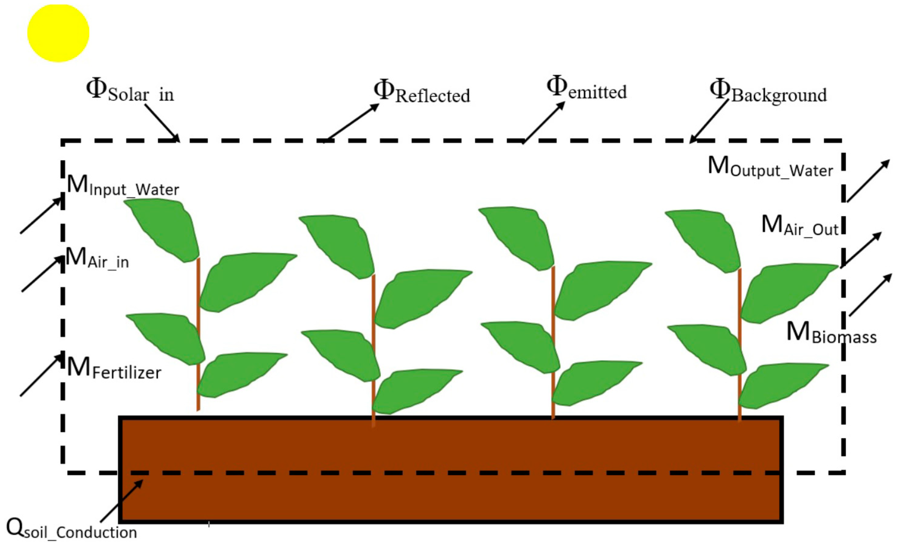
1.3. Energy and Exergy Analysis Applied to a Crop Plant System

The exergy destruction principle depends upon a black-box concept of engineering thermodynamics to assess how surface temperature can be used to characterize the energy flow of a crop plant system. A crop plant system is a complex open thermodynamic system that exchanges energy and matter with its surroundings. From an engineering thermodynamic perspective, a crop plant system can be modeled as a thermodynamic black box with input, output, and mass flows [50], as presented in Figure 2. For the mass flow, the input water is through the soil and rain/watering, the output water is through evaporation from the soil and evapotranspiration from the corn plant surface, the fertilizer input is through discrete applications at specified times, and the mass outputs as a biomass. Air flowing in and out of the system will carry water vapor in the form of humidity, while the soil may conduct thermal energy in or out of the system. When solar radiation reaches the crop surface, it will be absorbed or reflected. Furthermore, the background radiation comes from the radiation emitted from particles and molecules in the atmosphere and surrounding objects.
After conducting energy balance by using First and Second Laws of thermodynamics (referring to Figure 2), it is concluded that the radiation (i.e., incoming solar, reflected, background, and emitted radiation) and the transpiration terms dominate the other energy balance terms. On the other hand, for the exergy analysis, it was found that surface temperature can be used as a sole measurement for the net exergy available to a crop plant system [59]. The rate of exergy change in the system equals the rate of exergy input minus the rate of exergy output minus the rate of exergy destroyed [23,24]. It was found that the solar exergy dominates all other exergy input and output terms, with most of the solar exergy being destroyed or used by the system in one manner or another, for example, for photosynthesis and transpiration processes. The solar exergy can only be changed by changing the surface temperature, assuming a constant solar temperature [24,59].

2. Materials and Methods

Greenhouse experiments were conducted at the University of Guelph, Ontario, Canada, from October 2015 to February 2016. A single seed of corn hybrid Pioneer P8906AM was planted at a depth of 2 cm in the center of 180 individual pots (22.86 cm width, 22.54 cm depth) of 5.62 liters in volume and took approximately one week to emerge. The soil mixture was Turface® MVP (Profile Products LLC, Buffalo Grove, IL, USA). The pots were placed onto six separate benches, with each bench consisting of 30 pots (i.e., 6 pots wide × 5 pots in length), as illustrated in Figure 3. The experimental design was a randomized complete block design, which is similar to the experimental design used under field experiments with replications for the measurements error calculation. The experimental setup is shown in Figure 4. Two benches were assigned as independent individual replicates per nitrogen treatment. The pots had holes at the bottom, to allow for adequate drainage.
Two experiments were conducted from October 2015 to February 2016, to study the effect of varying nitrogen rate on surface temperature. Three rates of nitrogen (N), namely high (0.6 g N pot−1 or 160 kg ha−1), medium (0.3 g N pot−1 or 90 kg ha−1), and low (0.1 g N pot−1 or 30 kg ha−1), were applied to individual pots right after corn seed emergence, as described in Echarte et al. [60]. The nitrogen recipe that was used in the experiments is summarized in Table 1. The highest nitrogen rate of 160 kg ha−1 is set within the commercial rate applied for field corn production (personal communication, Swanton), while the other two rates (i.e., 90 and 30 kg ha−1) were chosen to ensure that differences in plant growth and development can be clearly observed under controlled environmental conditions.
The variability in surface temperature measurements between days is the result of many surrounding and weather-dependent variables that interact with leaf surface temperature, such as solar irradiance, air temperature, wind speed, relative humidity, atmospheric pressure, leaf angle, stomatal conductance, and leaf emissivity. Therefore, it is important to note that, in order to apply the EDP, corn plants with different N rates must be compared under the same environmental conditions, and this was achieved by growing all different supplied nitrogen rate crops within the same greenhouse at the same time. To minimize the leaf angle effect, the average leaf temperatures were used for analysis. A minimum effect on changing leaf surface temperature was observed for air temperatures within a range of 15–35 °C, assuming that other factors are held constant under controlled environmental conditions [61]. The measured average air temperature in the greenhouse was 24 ± 1.2 °C and 20 ± 0.4 °C during the day and night cycle, respectively.
Corn plants were hand-harvested around the seven leaf collar (V7) stage and then dried in an oven for 5 days, at 80 °C as the set temperature. The biomass of the dried corn (stem, leaves, and root) was measured by using a digital scale, which was calibrated manually before every measurement. Visual differences were observed between nitrogen treatments in plant height, leaf color, and root configuration. Corn leaf stage and plant height were recorded 2 to 3 times per week, to ensure that corn plants were growing and developing properly with respect to the applied rates of nitrogen.

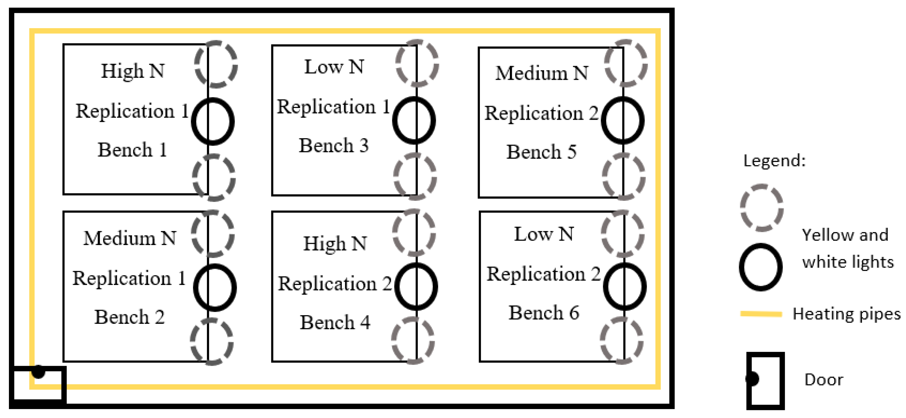
2.1. Experimental Design

The first experiment was conducted on 20 October 2015 and harvested on 27 November 2015, while the second experiment was conducted on 6 January 2016 and harvested on 2 February 2016. Both experiments were conducted under controlled conditions of air temperature, lighting, and water supply.
Nutrients were mixed with water and supplied automatically, right after seed emergence, to each bench separately, using a miniDos pump (Hydro systems, Cincinnati, OH, USA) connected to a timer. Nutrients and water were supplied to each pot individually, using a drip irrigation system. Each pot was supplied with an average of 2.5 cm water per week. In addition, weeds were manually removed from pots at the time of seed emergence, to ensure that corn plants were under nitrogen stress only. The light source in the greenhouse was set to supply a 16 h photoperiod. Two types of non-dimmable lamps were used: a 1000 Watt Metal Hallide lamp (SYLVANIA 64469-3, Gerrie Electric, Burlington, ON, Canada) and 1000 Watt High pressure sodium lamps (Gerrie Electric, Burlington, ON, Canada). There were 18 lamps of each type, alternating in 6 rows of 6. The light intensity at bench level was between 575 and 780 umol m−2 s−1. Lights were controlled with an ARGUS Control System.
The lighting system was GPS based, with a light meter to coordinate when the lights were fully on, half on, or completely off, depending on the outside weather conditions. Two fans were used for air circulation inside the experimental room. Air temperature was measured by using the Argus Greenhouse Management System (Argus Control System, Surrey, BC, Canada), which was recorded every 15 min. The sensors were protected in a metal hanging box in the middle of the experimental room, to minimize the errors associated with solar radiation and moisture.

2.2. Thermal Image Acquisition and Processing

An infrared thermal camera (T620, FLIR Systems, Burlington, ON, Canada) was used for leaf surface temperature measurements, at a sampling rate of twice per week. Leaf surface temperature measurements were initiated at second leaf collar (V2) stage and collected from the middle two rows, to avoid border effects. The technical specifications of the thermal camera are described in Table 2. The thermal camera has a precision of 0.1 °C. The thermal camera was manually calibrated by using the non-uniformity correction (NUC) button before every measurement. The NUC involves the selection of a calibration function to minimize the pixel variation caused by the charge buildup on the uncooled thermal detector [62]. Furthermore, the thermal camera was calibrated under laboratory conditions, using a blackbody source (463 cavity black-body, Infrared industries, Hayward, CA, USA) with a 2.2 cm diameter selected measurement aperture. The difference between the temperature obtained by the thermal camera and the temperature obtained by using the black-body cavity was no more than the accuracy of the thermal camera (±2 °C) [63].
The sample size for each experiment was randomly selected as 10 corn plants in the middle two rows out of 30 plants per bench, to avoid border effects. Temperature measurements were taken on the top (sunlight side) of fully expanded leaves. Corn leaf emissivity was set to 0.96, which was the average emissivity measured by using a Fourier Transform Infrared (FTIR) reflectometer (Surface Optics Corporation, San Diego, CA, USA), under laboratory conditions, averaged over the 7.5–14 µm wavelength band.
Thermal images were collected, using a FLIR T620 thermal camera; 10 images were collected from each bench, with a total of 20 images per nitrogen treatment. Thermal images were analyzed by using a ResearchIR (version 3.5, FLIR, Waterloo, ON, Canada) and Matlab software R2017b (Mathworks Inc., Natick, MA, USA), using an image processing toolbox. Average leaf temperatures were extracted and corrected for the variations in air temperature. The corrected leaf temperature was calculated by subtracting the measured leaf temperature from the measured air temperature acquired at the same time, then adding the average measured air temperature during leaf temperature measurements interval within a specific day. Temperature measurements were conducted consistently around noon, because the incoming solar radiation was then at maximum and would not change much during temperature measurements [64]. Sunny and uniform overcast days were chosen for temperature data acquisition for a uniform-sky-background radiation assumption.
An infrared (IR) handheld point measurement gun (maximum infrared thermometer, Whitehorse, YT, Canada) was also used for leaf surface temperature measurements (due to small test area), on a daily basis, over an average of 10 days per experiment. The IR gun was held at 0.5 m and at a 90° angle away from the leaf surface, to minimize the reflection and background radiation effects [65]. In addition, whorl temperatures were measured by using a type T, ungrounded with FEP-Insulated, thermocouple. The chosen thermocouples were manufactured by Digi-Sense, Canada, with Tmax = 400 °C, and 0.51 mm in diameter. Thermocouples were attached through a mini connector to a 12 channel data-logging thermometer with a security digital card (Extech DT4208SD, Cole-Parmer, Montreal, QC, Canada), for continuous temperature measurements, with a sampling rate of 30 min, and whorl temperature averages were recorded. Thermocouples were placed directly into the whorl of corn plants, to minimize the error associated with heat radiation.

2.3. Data Analysis

Statistical data analysis was conducted by using Matlab software. Analysis of variance (ANOVA) and F-test were utilized to test the significance of decreasing surface temperature with increasing rates of nitrogen, using the anova1 function in Matlab. In addition, Tukey’s post hoc test was used to find which specific treatment means (compared with each other) were different. Moreover, t-test at p < 0.05 was used to test the significant difference between low and high nitrogen treatments, and the mean leaf temperatures were compared over different treatments and tested for significance, as presented in Table 3. A p-value < 0.05 confirmed the significant difference in temperatures among nitrogen treatments.

3. Results

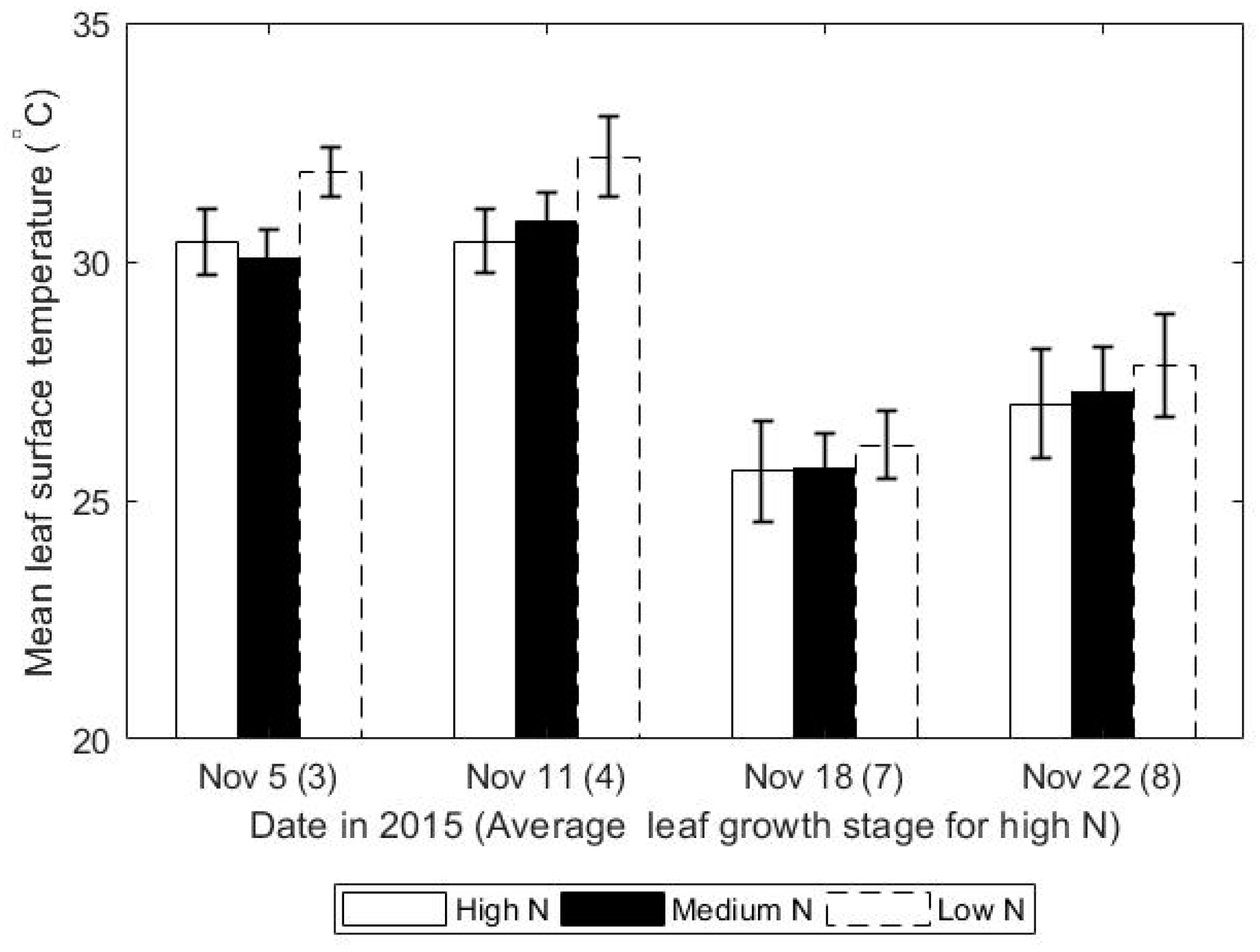
3.1. Leaf Surface Temperature Decreased with Increasing Rates of Nitrogen

Leaf surface temperature decreased with increasing rates of nitrogen. The mean leaf surface temperatures, measured by using an IR handheld gun for corn receiving high, medium, and low nitrogen rates on 9 November 2015, were 25.48 ± 2.59 °C, 25.55 ± 1.94 °C, and 28.74 ± 3.43 °C, respectively, with a corresponding statistically significant difference among nitrogen treatments. A p-value of less than 0.05 confirmed the significant difference in the mean leaf temperatures among nitrogen treatments (Table 4). Leaf surface temperature associated with high, medium, and low nitrogen rates is presented as mean ± SD in Table 4 for different days. The mean leaf surface temperatures, measured by using a thermal camera for corn receiving high, medium, and low nitrogen rates on 29 January 2016, were 23.82 ± 1.75 °C, 24.44 ± 0.96 °C, and 24.08 ± 1.2 °C, respectively (Table 5). A consistent decrease in leaf surface temperature was observed with increasing rates of nitrogen (Figure 5). On 11 November 2015, the mean leaf temperatures, measured by using a thermal camera for corn receiving high, medium, and low rates of nitrogen, were 30.43 ± 1.0 °C, 30.82 ± 0.68 °C, and 32.19 ± 1.12 °C, respectively (Figure 6), where the error bars represent the variability in leaf temperature. A consistent significant decrease in leaf surface temperature was observed on different days at the 0.05 significance level.

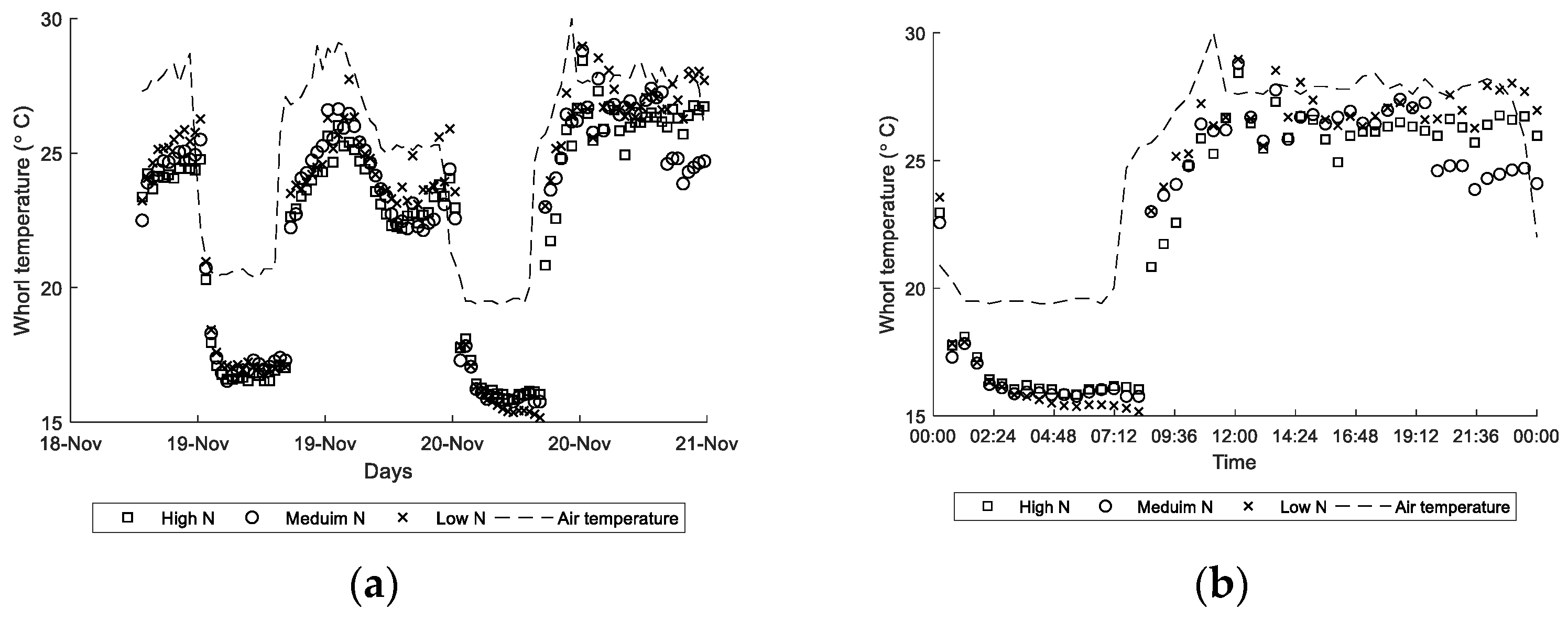
3.2. Whorl Temperature Variation between Day and Night

Whorl temperatures were proposed as a proxy for surface temperature, to investigate the effect of nitrogen stress on temporal surface temperature variation during the day and night. Whorl temperatures were measured by using type T thermocouples inserted into the whorl of stressed and less stressed corn plants, during the day and night cycle, to investigate if there was a significant difference. It was observed that less-stressed corn plants during the day have cooler whorl temperatures when compared to stressed plants (Figure 7). During the night, less-stressed plants were hotter when compared to nitrogen-stressed plants, a finding which was expected when there is no energy input from solar radiation, and the more developed and less stressed crop system should be more conservative in energy use, thus having higher temperatures at night [66]. Figure 7a,b presents the diurnal variation in whorl temperatures over three days and a one-day period, respectively.
It is valuable to note that the warmer air temperature relative to whorl temperature at night, presented in Figure 7b, was not unexpected, given that the measurements shown were taken under greenhouse conditions in fall, November 2015, where the air temperature in the room was heated, while the greenhouse walls and ceiling were cold due to the colder outdoor temperature. That is, a cooler whorl temperature confirms a situation where the heat loss to the background controls the energy balance at the plant surface, similar to when a background radiation controls the formation of frost on lawns at night. The question then arises, when analyzing whorl temperatures at night, if temperature difference trends between plants under different nitrogen stress levels are the result of nitrogen stress, or because of changes in energy balance given there is no solar radiation input at night. Moreover, the warmer nitrogen-stressed plants will initially cool faster, compared to less stressed plants, due to the large temperature difference between plant surface temperature and background radiation temperature. The physics of radiation heat transfer dictates, that for the stressed plants to cool to a lower temperature compared to less stressed plants at night, stressed plants must have properties or mechanisms unrelated to the incoming background radiation that differ from the non-stressed plants. One possible reason mirrors what happens in a desert, where temperatures fluctuate widely between day and night [67], due to low “effective” thermal mass.

3.3. Biomass Increased with Increasing Rates of Nitrogen and Leaf Surface Temperature Decreased

The total biomass of corn increased with increasing rates of nitrogen, while surface temperature decreased. The mean total biomass (10 corn plants per bench) from leaves, stem, and roots was higher in corn receiving higher rates of nitrogen, compared to corn receiving lower rates of nitrogen (Table 6). The mean total biomass of 20 measurements per nitrogen treatment in corn receiving high, medium, and low rates of nitrogen in the first experiment was 18.9 ± 3.49 g, 11.1 ± 1.92 g, and 6.5 ± 1.34 g, respectively. In the second experiment, the mean total biomass for corn receiving high, medium, and low rates of nitrogen was 4.4 ± 0.97 g, 4.2 ± 1.17 g, and 3.3 ± 0.61 g, respectively. There was a substantial difference in the two experiments, due to leaf-stage difference at harvest time. On 27 November 2015, corn plants that received high, medium, and low rates of nitrogen were in 11, 9, and 9 average leaf tip stage, respectively, at harvest time, and on 2 February 2016, corn plants that received high, medium, and low rates of nitrogen were in 8, 7, and 7 average leaf tip stage, respectively, at the harvest time.

4. Discussion

An inverse relationship was found between plant growth/development, nitrogen stress, and leaf temperature [65] under variable field conditions, thus providing experimental support for the exergy destruction principle (EDP). The EDP implies that more complex and developed ecosystems should be more efficient in energy dissipation and exergy degradation, as compared to less complex and less developed ecosystems; thus, their surface temperatures decrease [31,32,33,38,41,42,43,44,65,66]. Ecosystems develop in a way that maintains their ability to survive, while increasing the ability to extract the solar exergy and utilize it to maintain their organization. Luvall et al. [44,45,46] showed that, under the same environmental conditions, the more developed the ecosystem, the colder its surface temperature and more degraded its emitted energy. In this study, it was expected that corn plants receiving higher/optimum rates of nitrogen would be more developed and able to destroy more exergy from the incoming radiation, as compared to stressed corn plants under the same environmental conditions. The degree to which the incoming solar exergy is destroyed is a function of surface temperature. Assuming that corn plants received the same amount of incoming radiation, it is expected that less-stressed corn plants will emit energy at a lower quality level, thus lowering their surface temperature. The EDP suggests that a less stressed crop system will reject or lose less exergy in the form of thermal radiation, compared to stressed crop systems; hence, it will have a lower surface temperature during the day that inherently radiates less energy (at a given emissivity). Otherwise, stress will affect the plants ability to efficiently utilize and destroy the solar exergy during the day, and its surface temperature increases [50].
This work summarizes the two experiments conducted under the greenhouse conditions, to test and justify the hypothesis that corn crops supplied with optimum or high rates of nitrogen will have lower surface temperatures when compared to corn grown under nitrogen-stressed conditions, as predicted by the exergy destruction principle. The greenhouse environment was used as a proxy for the field environment, and leaf surface temperature was used as a proxy representing canopy temperature.
The inverse surface temperature correlation with nitrogen stress presented in this paper has the potential to lead to the use of thermal imaging to precisely and optimally apply nitrogen fertilizer to a crop plant: precise in location, and optimal in amount, which will subsequently increase the yield, reduce supplied fertilizer costs, and reduce the harmful impacts of fertilizer runoff on the environment. Furthermore, it may, in the future, be shown that crop stress due to weeds or pests will also find thermal imaging beneficial to precision agriculture application of herbicides and pesticides to crop plants.

5. Conclusions

The results obtained from this study support the proposed hypothesis that nitrogen-stressed corn plants will have higher temperatures during the day and less biomass, as compared to less-stressed corn plants. In this study, an approximate 2 °C difference was observed in leaf temperatures between corn receiving high and low rates of nitrogen at different growth stages. In this work, the proxy between greenhouse and field environments was established for the purpose of applying the exergy destruction principle, where leaf surface temperature was used as a proxy for canopy temperature. In addition, it was observed that nitrogen-stressed plants have higher whorl temperatures during the day and lower whorl temperatures during the night, compared to less-stressed plants. Therefore, more extensive studies on the relationship between whorl/leaf temperature, both day and night, are recommended to be conducted as a means to better understand how the exergy destruction principle (EDP) relates to the overall energy balance of a crop plant system, and not just how it relates when plants are photosynthesis active (around solar noon). As a recommendation, future work will refine the conditional sampling conducted in this work; for example, in addition to taking measurements around solar noon, measurements could be sorted by an incoming solar intensity, at the time of temperature measurement.

Author Contributions

H.A., R.F., and C.S. contributed to hypothesis formulation of the research, analyzing and discussing the results, and manuscript writing. All authors have read and agreed to the published version of the manuscript.

Funding

This research was undertaken in part with funding from the Canada First Research Excellence Fund and through Growing Forward 2 (GF2), a federal–provincial–territorial initiative. The Agricultural Adaptation Council assists in the delivery of GF2 in Ontario, Canada. The authors would also like to acknowledge the support of the Natural Sciences and Engineering Research Council of Canada (NSERC).

Institutional Review Board Statement

Not Applicable.

Informed Consent Statement

Not Applicable.

Data Availability Statement

Data sharing not applicable.

Acknowledgments

This research was undertaken in part with funding from the Canada First Research Excellence Fund and through Growing Forward 2 (GF2), a federal–provincial–territorial initiative. The Agricultural Adaptation Council assists in the delivery of GF2 in Ontario, Canada. The authors would also like to acknowledge the support of the Natural Sciences and Engineering Research Council of Canada (NSERC). Furthermore, the authors would like to thank the staff from the University of Guelph, ON, Canada, for providing the required facilities and equipment for conducting the experiments under greenhouse conditions.

Conflicts of Interest

The authors declare no conflict of interest.

References

  1. Leff, B.; Ramankutty, N.; Foley, J.A. Geographic distribution of major crops across the world. Glob. Biogeochem. Cycles 2004, 18. [Google Scholar] [CrossRef]
  2. Subedi, K.D.; Ma, B.L. Assessment of some major yield-limiting factors on maize production in a humid temperate environment. Field Crops Res. 2009, 110, 21–26. [Google Scholar] [CrossRef]
  3. Verma, D.; Pareek, N. Study of Broiling effect on Nutritional Quality and Phytochemical Content in Sweet Corn. Int. J. Environ. Rehabil. Conserv. 2018, 158–188. [Google Scholar] [CrossRef]
  4. Serna-Saldivar, S.O.; Carrillo, E.P. Food uses of whole corn and dry-milled fractions. In Corn; AACC International Press: St. Paul, MN, USA, 2019; pp. 435–467. [Google Scholar]
  5. Shapiro, C.A.; Wortmann, C.S. Corn response to nitrogen rate, row spacing, and plant density in eastern Nebraska. Agron. J. 2006, 98, 529–535. [Google Scholar] [CrossRef] [Green Version]
  6. Montezano, Z.F.; Corazza, E.J.; Muraoka, T. Variabilidade de nutrientes em plantas de milho cultivado em talhão manejado homogeneamente. Bragantia 2008, 67, 969–976. [Google Scholar] [CrossRef] [Green Version]
  7. Blackmer, T.M.; Schepers, J.S. Aerial photography to detect nitrogen stress in corn. J. Plant Physiol. 1996, 148, 440–444. [Google Scholar] [CrossRef]
  8. Meyer, J. Sugarcane nutrition and fertilization. In Good Management Practices Manual for the Cane Sugar Industry; Meyer, J., Ed.; The International Finance Corporation (IFC): Johannesburg, South Africa, 2011; pp. 173–226. [Google Scholar]
  9. Ni, Z.; Liu, Z.; Huo, H.; Li, Z.L.; Nerry, F.; Wang, Q.; Li, X. Early water stress detection using leaf-level measurements of chlorophyll fluorescence and temperature data. Remote Sens. 2015, 7, 3232–3249. [Google Scholar] [CrossRef] [Green Version]
  10. Rhezali, A.; Lahlali, R. Nitrogen (N) mineral nutrition and imaging sensors for determining N status and requirements of maize. J. Imaging 2017, 3, 51. [Google Scholar] [CrossRef] [Green Version]
  11. Bongiovanni, R.; Lowenberg-DeBoer, J. Precision agriculture and sustainability. Precis. Agric. 2004, 5, 359–387. [Google Scholar] [CrossRef]
  12. Valentin, A.S.R.; Horstrand, P.; López, J.F.; López, S. Setting up an autonomous hyperspectral flying platform for precision agriculture. In High-Performance Computing in Geoscience and Remote Sensing, International Society for Optics and Photonics; SPIE: Berlin, Germany, 2018; Volume 10792, p. 1079206. [Google Scholar]
  13. Muñoz-Huerta, R.F.; Guevara-Gonzalez, R.G.; Contreras-Medina, L.M.; Torres-Pacheco, I.; Prado-Olivarez, J.; Ocampo-Velazquez, R.V. A review of methods for sensing the nitrogen status in plants: Advantages, disadvantages and recent advances. Sensors 2013, 13, 10823–10843. [Google Scholar] [CrossRef]
  14. Paleari, L.; Movedi, E.; Vesely, F.M.; Thoelke, W.; Tartarini, S.; Foi, M.; Confalonieri, R. Estimating crop nutritional status using smart apps to support nitrogen fertilization. A case study on paddy rice. Sensors 2019, 19, 981. [Google Scholar] [CrossRef] [PubMed] [Green Version]
  15. Xiong, D.; Chen, J.; Yu, T.; Gao, W.; Ling, X.; Li, Y.; Huang, J. SPAD-based leaf nitrogen estimation is impacted by environmental factors and crop leaf characteristics. Sci. Rep. 2015, 5, 13389. [Google Scholar] [CrossRef] [PubMed] [Green Version]
  16. Zhang, J.; Blackmer, A.M.; Blackmer, T.M. Reliability of chlorophyll meter measurements prior to corn silking as affected by the leaf change problem. Commun. Soil Sci. Plant Anal. 2009, 40, 2087–2093. [Google Scholar] [CrossRef]
  17. Maes, W.H.; Steppe, K. Perspectives for remote sensing with unmanned aerial vehicles in precision agriculture. Trends Plant Sci. 2019, 24, 152–164. [Google Scholar] [CrossRef] [PubMed]
  18. Jackson, R.D.; Idso, S.B.; Reginato, R.J.; Pinter, P.J., Jr. Canopy temperature as a crop water stress indicator. Water Resour. Res. 1981, 17, 1133–1138. [Google Scholar] [CrossRef]
  19. Abraham, N.; Hema, P.S.; Saritha, E.K.; Subramannian, S. Irrigation automation based on soil electrical conductivity and leaf temperature. Agric. Water Manag. 2000, 45, 145–157. [Google Scholar] [CrossRef]
  20. Jones, H.G.; Rotenberg, E. Energy, radiation and temperature regulation in plants. In eLS; Wiley: New York, NY, USA, 2001. [Google Scholar]
  21. Unkovich, M.; Baldock, J.; Farquharson, R. Field measurements of bare soil evaporation and crop transpiration, and transpiration efficiency, for rainfed grain crops in Australia—A review. Agric. Water Manag. 2018, 205, 72–80. [Google Scholar] [CrossRef]
  22. Kokin, E.; Palge, V.; Pennar, M.; Jürjenson, K. Strawberry leaf surface temperature dynamics measured by thermal camera in night frost conditions. Agron. Res. 2018, 16. [Google Scholar] [CrossRef]
  23. Cangel, Y.A.; Boles, M.A. Thermodynamics: An Engineering Approach, 4th ed.; McGraw-Hill: Singapore, 2002. [Google Scholar]
  24. Fraser, R.; Kay, J.J. Exergy analysis of ecosystems: Establishing a role for thermal remote sensing. In Thermal Remote Sensing in Land Surface Processing; Taylor and Francis: London, UK, 2004; pp. 283–360. [Google Scholar]
  25. Kotas, T.J. The Exergy Method of Thermal Plant Analysis; Elsevier: Amsterdam, The Netherlands, 2013. [Google Scholar]
  26. Cornelissen, R. Thermodynamics and Sustainable Development: The Use of Exergy Analysis and the Reduction of Irreversibility. Ph.D. Thesis, University of Groningen, Groningen, The Netherland, 1999. [Google Scholar]
  27. Cornelissen, R.L.; Hirs, G. The value of the exergetic life cycle assessment besides the LCA. Energy Convers. Manag. 2002, 43, 1417–1424. [Google Scholar] [CrossRef]
  28. Wall, G. Exergy a useful concept within resource accounting. In Chalmers Tekniska Högskola; Göteborgs Universitet: Gothenburg, Sweden, 1977. [Google Scholar]
  29. Wall, G. Exergy conversion in the Swedish society. Resour. Energy Econ. 1987, 9, 55–73. [Google Scholar] [CrossRef] [Green Version]
  30. Wall, G. Exergy conversion in the Japanese society. Energy 1990, 15, 435–444. [Google Scholar] [CrossRef]
  31. Kay, J.J.; Schneider, E.D. Thermodynamics and measures of ecological integrity. In Ecological Indicators; Springer: Boston, MA, USA, 1992; pp. 159–182. [Google Scholar]
  32. Schneider, E.D.; Kay, J.J. Complexity and thermodynamics: Towards a new ecology. Futures 1994, 26, 626–647. [Google Scholar] [CrossRef]
  33. Schneider, E.D.; Kay, J.J. Life as a manifestation of the second law of thermodynamics. Math. Comput. Model. 1994, 19, 25–48. [Google Scholar] [CrossRef]
  34. Schrodinger, E. What Is Life?: With Mind and Matter and Autobiographical Sketches; Cambridge University Press: Cambridge, UK, 2012. [Google Scholar]
  35. Jørgensen, S.E.; Nielsen, S.N. Application of exergy as thermodynamic indicator in ecology. Energy 2007, 32, 673–685. [Google Scholar] [CrossRef]
  36. Gong, M.; Wall, G. On exergy and sustainable development-Part 2: Indicators and methods. Exergy Int. J. 2001, 1, 217–233. [Google Scholar] [CrossRef]
  37. Maes, W.H.; Pashuysen, T.; Trabucco, A.; Veroustraete, F.; Muys, B. Does energy dissipation increase with ecosystem succession? Testing the ecosystem exergy theory combining theoretical simulations and thermal remote sensing observations. Ecol. Model. 2011, 222, 3917–3941. [Google Scholar] [CrossRef]
  38. Kay, J.J. Ecosystems as self-organizing holarchic open systems: Narratives and the second law of thermodynamics. In Handbook of Ecosystem Theories and Management; Lewis Publishers: Boca Raton, FL, USA, 2000. [Google Scholar]
  39. Prigogine, I. Etude Thermodynamique des Phe’nome`nes Irre´- Versibles; Desoer: Liege, Belgium, 1947. [Google Scholar]
  40. Nicolis, G.; Prigogine, I. Exploring Complexity: An Introduction; Freeman: New York, NY, USA, 1989. [Google Scholar]
  41. Luvall, J.C.; Quattrochi, D.A. Thermal characteristics of urban landscapes. In Proceedings of the 23rd Conference on Agricultural and Forest Meteorology, Albuquerque, NM, USA, 2–6 November 1998. [Google Scholar]
  42. Luvall, J.C.; Rickman, D.; Fraser, R.F. Thermal remote sensing and the thermodynamics of ecosystem development. In Proceedings of the AGU Fall Meeting 2013, San Francisco, CA, USA, 9–13 December 2013. [Google Scholar]
  43. Kay, J.J.; Allen, T.; Fraser, R.; Luvall, J.C.; Ulanowicz, R. Can we use energy based indicators to characterize and measure the status of ecosystems, human, disturbed and natural. In Proceedings of the International Workshop: Advances in Energy Studies: Exploring Supplies, Constraints and Strategies, Porto Venere, Italy, 19–21 October 2001; pp. 121–133. [Google Scholar]
  44. Luvall, J.C.; Holbo, H.R. Measurements of short-term thermal responses of coniferous forest canopies using thermal scanner data. Remote Sens. Environ. 1989, 27, 1–10. [Google Scholar] [CrossRef]
  45. Luvall, J.C.; Holbo, H.R. Thermal remote sensing methods in landscape ecology. Ecol. Stud. 1991, 82, 127–152. [Google Scholar]
  46. Quattrochi, D.A.; Luvall, J.C. Thermal infrared remote sensing for analysis of landscape ecological processes: Methods and applications. Landsc. Ecol. 1999, 14, 577–598. [Google Scholar] [CrossRef]
  47. Quattrochi, D.A.; Luvall, J.C. Thermal Remote Sensing in Land Surface Processing; CRC Press: Boca Raton, FL, USA, 2004. [Google Scholar]
  48. Lin, H.; Zhang, H.; Song, Q. Transition from abstract thermodynamic concepts to perceivable ecological indicators. Ecol. Indic. 2018, 88, 37–42. [Google Scholar] [CrossRef]
  49. Holdaway, R.J.; Sparrow, A.D.; Coomes, D.A. Trends in entropy production during ecosystem development in the Amazon Basin. Philos. Trans. R. Soc. B Biol. Sci. 2010, 365, 1437–1447. [Google Scholar] [CrossRef] [PubMed] [Green Version]
  50. Lawrence, R. Thermal Remote Sensing and the Exergy Destruction Principle Applied to Precision Agriculture. Master’s Thesis, University of Waterloo, Waterloo, ON, Canada, 2016. [Google Scholar]
  51. Duncan, W.G.; Hatfield, A.L.; Ragland, J.L. The growth and yield of corn II: Daily growth of corn kernels. Agron. J. 1965, 57, 221–223. [Google Scholar] [CrossRef]
  52. Nunez, R.; Kamprath, E. Relationships between N response, plant population, and row width on growth and yield of corn. Agron. J. 1969, 61, 279–282. [Google Scholar] [CrossRef]
  53. Finn, J.T. RE Ulanowicz: Growth and development: Ecosystems phenomenology. Behav. Sci. 1988, 33, 158–159. [Google Scholar] [CrossRef]
  54. Reiniger, P.; Seguin, B. Surface temperature as an indicator of evapotranspiration and soil moisture. Remote Sens. Rev. 1986, 1, 277–310. [Google Scholar] [CrossRef]
  55. Mamo, M.; Malzer, G.L.; Mulla, D.J.; Huggins, D.R.; Strock, J. Spatial and temporal variation in economically optimum nitrogen rate for corn. Agron. J. 2003, 95, 958–964. [Google Scholar] [CrossRef] [Green Version]
  56. McDonald, A.; Davies, W.J. Keeping in touch: Responses of the whole plant to deficits. Adv. Bot. Res. 1996, 22, 229. [Google Scholar]
  57. Reddy, T.Y.; Reddy, V.R.; Anbumozhi, V. Physiological responses of groundnut (Arachis hypogea L.) to drought stress and its amelioration: A critical review. Plant Growth Regul. 2003, 41, 75–88. [Google Scholar] [CrossRef]
  58. Pirasteh-Anosheh, H.; Saed-Moucheshi, A.; Pakniyat, H.; Pessarakli, M. Stomatal responses to drought stress. Water Stress Crop Plants 2016, 24–40. [Google Scholar] [CrossRef]
  59. Alzaben, H. Investigating the Exergy Destruction Principle Applied to Precision Agriculture Using Thermal Remote Sensing. Ph.D. Thesis, University of Waterloo, Waterloo, ON, Canada, 2020. [Google Scholar]
  60. Echarte, L.; Rothstein, S.; Tollenaar, M. The response of leaf photosynthesis and dry matter accumulation to nitrogen supply in an older and a newer maize hybrid. Crop Sci. 2008, 48, 656–665. [Google Scholar] [CrossRef]
  61. Nelson, J.A.; Bugbee, B. Analysis of environmental effects on leaf temperature under sunlight, high pressure sodium and light emitting diodes. PLoS ONE 2015, 10, e0138930. [Google Scholar] [CrossRef] [PubMed]
  62. Niklaus, F.; Vieider, C.; Jakobsen, H. MEMS-based uncooled infrared bolometer arrays: A review. In MEMS/MOEMS Technologies and Applications; International Society for Optics and Photonics: San Diego, CA, USA, 2008; Volume 6836, p. 68360D. [Google Scholar]
  63. Alzaben, H.; Fraser, R.; Swanton, C. An inverse correlation between corn temperature and nitrogen stress: A field case study. Agron. J. 2019, 111, 3207–3219. [Google Scholar] [CrossRef]
  64. Mury, A. The Light Field in Natural Scenes. Master’s Thesis, University of Delft, Delft, The Netherlands, 2009. [Google Scholar]
  65. Akbari, M.H. Energy-Based Indicators of Ecosystem Health. Master’s Thesis, University of Guelph, Guelph, ON, Canada, 1996. [Google Scholar]
  66. Safty, M.E. Use and organization of domestic space in the Arab world. Int. J. Sociol. Fam. 1981, 11, 179–199. [Google Scholar]
  67. Song, D.; Bhushan, B. Bioinspired triangular patterns for water collection from fog. Philos. Trans. R. Soc. 2019, 377, 20190128. [Google Scholar] [CrossRef] [PubMed] [Green Version]
Figure 1. The selected system boundary under (a) field and (b) greenhouse. (c) Crop system boundary surrounds multiple plants and roots, encompassing soil and surrounding air in the field. (d) A proxy of crop system boundary surrounds multiple plants, roots, and pots, encompassing soil and surrounding air in the greenhouse.
Agriculture 11 00101 g001
Figure 2. Mass and energy flows of a crop plant system [59].
Agriculture 11 00101 g002
Figure 3. Greenhouse layout (this picture was taken on 5 November 2015).
Agriculture 11 00101 g003
Figure 4. The experimental setup conducted in the greenhouse.
Agriculture 11 00101 g004
Figure 5. The inverse correlation between nitrogen rate and leaf surface temperature in the two experiments conducted under greenhouse conditions when three rates of nitrogen (low (L), medium (M), and high (H)) were supplied (2 nitrogen treatments × 10 data points/treatment × 2 experiments = 40 data points per treatment).
Agriculture 11 00101 g005
Figure 6. The mean leaf surface temperature decreases with nitrogen rate increase, as seen by using the thermal camera data in the first experiment conducted in the greenhouse.
Agriculture 11 00101 g006
Figure 7. Whorl temperature variations between day and night in November 2015 over (a) three days and (b) a one-day period.
Agriculture 11 00101 g007
Table 1. The nitrogen recipe used for corn plants.
For N ControlHigh N (20 mM) (kg)Medium N (12 mM) (kg)Low N (4 mM)
(kg)
34-0-016.479.883.29
HPO43.743.743.74
KHCO3 (0-0-47)7.57.57.5
MgSO4 7H2O888
Micronutrient (pH 5.6–6.0)0.60.60.6
Table 2. The specifications of FLIR T-620 thermal camera.
FeaturesSpecifications
Resolution640 × 480 pixels
Temperature range−40 to 650 °C
Spectral range7.5–14 μm
Thermal sensitivity<0.04 °C at 30 °C
Minimum focus distance0.25 m
Image frequency (frame rate)30 Hz
Accuracy±2 °C
Field of view25 × 190
Table 3. ANOVA analysis on the mean leaf surface temperature data extracted from the first experiment, using IR handheld gun data.
Source SS a df b MS c Fcalcu d Fcriti ep-Value
N rate14672733.3418.163.023.46 × 10−4
Error12,59831240.38
Total 14,065314
Where a is the total sum of the squares which is related to the total variance in temperature data, b is the degree of freedom, c is the mean squared error which is produced by dividing SS over df, d is the calculated F value through dividing the mean square of regression (MSR) for N rate and days over the mean square of error (MSE), and e is the critical F value that is determined by using F-tables with a corresponding degree of freedom for numerator (mean square of regression (i.e., MSR)) and denominator (mean square of error (i.e., MSE)).
Table 4. The mean leaf temperature increases with nitrogen stress in the first experiment, using IR handheld gun data.
Date
in 2015
Leaf Tip Stage
a
High N b
(°C)
Medium N
(°C)
Low N
(°C)
p-Value c
3 November 29.63 ± 2.7626.82 ± 3.129.13 ± 2.060.003
5 November327.89 ± 1.8227.59 ± 2.3728.96 ± 2.090.057
6 November326.11 ± 1.4125.10 ±1.7129.19 ± 3.25<0.001
9 November425.48 ± 2.5925.55 ± 1.9428.74 ± 3.43<0.001
10 November429.61 ± 3.4830.63 ± 2.4533.81 ± 3.31<0.001
12 November523.10 ± 1.8524.38 ± 2.3225.92 ± 2.07<0.001
13 November523.33 ± 1.2523.44 ± 1.8726.83 ± 1.76<0.001
16 November631.03 ± 2.2727.88 ± 3.0432.25 ± 3.05<0.001
17 November726.10 ± 0.9522.65 ± 2.0925.23 ± 2.93<0.001
Where a is the average leaf tip stage for the high nitrogen rate corn plants on a specific day, b is the mean leaf temperatures presented as mean ± SD °C, and c is the p-value which refers to the level of significance among the three treatments calculated after averaging the temperature measurements from two replications on a specific day. The significance level was chosen as p ≤ 0.05.
Table 5. The mean leaf surface temperature increases with nitrogen stress in the two experiments conducted in the greenhouse, using the thermal camera data.
DateLeaf Tip StageHigh N
(°C)
Medium N
(°C)
Low N
(°C)
p-Value
2015
5 November330.41 ± 0.6830.08 ± 0.631.88 ± 0.52<0.001 a
11 November430.43 ± 0.4530.82 ± 0.4132.19 ± 0.730.005 a
18 November725.885 ± 1.4624.33 ± 1.1127.13 ± 1.83<0.001 a
22 November725.61 ± 1.0625.69 ± 0.7326.16 ± 0.710.39 b
24 November827.02 ± 1.3127.28 ± 0.8827.82 ± 1.330.1 b
2016
19 January324.45 ± 3.4924.29 ± 2.0725.46 ± 2.060.13 b
23 January424.93 ± 2.0424.52 ±1.1224.51 ± 1.710.35 b
29 January623.82 ± 1.7524.44 ± 0.9624.08 ± 1.20.3 b
Where “a” and “b” represent the statistical significance at p ≤ 0.05.
Table 6. The mean total biomass increases with nitrogen rate increase for the two experiments conducted in the greenhouse.
Experiment No.Time PeriodHigh N
(g)
Medium N
(g)
Low N
(g)
1October–December 201518.9 ± 3.4911.1 ± 1.926.5 ± 1.34
2January–February 20164.4 ± 0.974.2 ± 1.173.3 ± 0.61
Publisher’s Note: MDPI stays neutral with regard to jurisdictional claims in published maps and institutional affiliations.

