Abstract
The decision on crop population density should be a function of biotic and abiotic field parameters and optimize the site-specific yield potential, which can be a real challenge for farmers. The objective of this study was to investigate the yield of maize hybrids subjected to variable rate seeding (VRS) and in differentiated management zones (MZs). The experiment was conducted between 2013 and 2015 in a commercial field in the Central-West region of Brazil. First, MZ were delineated using the K-means algorithm with layers involving soil electrical conductivity, yield maps from previous years, and elevation. Seven maize hybrids at five seeding rates were evaluated in the context of each MZ and the cause-and-effect relationship with soil attributes was investigated. Optimal yields were obtained for crop population densities between 70,000 plants ha−1 and 80,000 plants ha−1. Hybrids which perform well under higher densities are key in achieving positive results using VRS. The plant population densities that resulted in maximum yields were obtained for densities at least 27% higher than the recommended seeding rates. The yield variance between MZs can be explained by the variance in soil attributes, while the yield variance within MZs can be explained by the variance in plant population densities. The study shows that on-farm experimentation can be key for obtaining information concerning yield potential. The management by VRS in different MZs is a low-cost technique that can reduce input application costs and optimize yield according to the site-specific potential of the field.
1. Introduction
The optimum plant density at which crop yield is maximized must consider the specificity of each environment []. Crop management strategies are a function of complex interactions between biotic and abiotic factors and can be a challenge for farmers to achieve better economic results. For example, the interaction between biotic and abiotic factors can reflect a crop’s spatial variability within the fields. Therefore, the adoption of precision agriculture techniques (PA) provides tools that help stakeholders address crop spatial variability [,]. For example, one possible strategy for managing the spatial variability of crops is the use of variable rate seeding (VRS) to optimize the use of environmental resources [].
Studies concerning the variability of seeding rates and spacing between rows have been carried out in experimental plots to evaluate the correlation between soil parameters and yield [,]. Coronel et al. [] evaluated maize yield at different sowing depths using management zones (MZs). In their study, MZs were delineated based on relative altitude data rather than spatial patterns of soil moisture. MZ delineation constitutes a management strategy that allows agricultural inputs to be allocated according to the yield potential of each zone. Nevertheless, the delineation of MZs relies on information layers that can be related to yield []. However, there is a lack of studies evaluating variable rate seeding in commercial fields using the MZ concept, i.e., for homogeneous regions with distinct yield potential.
The delimitation of MZs supports the management of spatial variability [] and allows for greater control of cause-and-effect relationships, e.g., to evaluate the increase in yield potential under specific conditions [,,,,,,]. MZs can help mitigate the unmanageable external effects and optimize the use of inputs, such as seeding, which could have optimal ranges for a determined zone. The development of the prescription map for an ideal application, aiming for reasonable management of the inputs, requires a deep understanding of in field variability. Such variability relies on the system interactions accounted for by soil, crop, weather, and management practices []. Therefore, different information namely stable soil properties and yield maps allows a representative delimitation of these effects on the expression of the yield potential. Through MZs, it is possible to evaluate different planting strategies, varying the seeding rate, as well as using different hybrids of the same crop, in search of optimal yields for the characteristics observed in the field. Kayad et al. [] and Miao et al. [] summarized that an efficient delineation of MZs should rely either on (i) crop yield maps, (ii) a stable soil attribute such as soil electric conductivity, or (iii) the combination of both.
Also considering similar layers as recommended by Kayad et al. [], Gavioli et al. [] assessed the outcome of several clustering algorithms on the delineation of MZs for precision agriculture. The authors report that most clustering algorithms were able to significantly reduce variance within MZs and provide zones with high internal homogeneity []. In addition, two to three MZs were enough to partition the field in areas of statistically distinct average yields.
Employing such management strategies to optimize yield using site-specific management of inputs, has been suggested as the most economically viable approach due to the possibility of using conventional agriculture equipment []. Aside from optimizing profit, MZs are generally adopted to reduce the excessive application of fertilizers and environmental impacts associated with it. However, MZs are often overlooked when it comes to variable rate seeding. Moreover, in addition to defining the MZs as a management strategy, it is essential to conduct on-farm experiments to reach the crop’s productive potential in each portion of the field and define the recommendation that provides the desired results for the activity [].
Concerning on-farm experimentation, Horbe et al. [] evaluated the efficiency of variable rate seeding for maize in MZs delineated based on the farmer’s knowledge and by overlapping yield data from nine grain crops (soybean and maize). The authors obtained higher yields in low-potential MZs by reducing the maize population relative to the recommended fixed population. In addition, they also achieved higher yields in high-potential MZs by increasing the plant population relative to the recommended fixed population. In general, the maize yield shows a quadratic response to plant population, allowing an optimum seeding rate to be determined from which the increase in total grain yield outweighs the reduction in yield per plant []. Horbe et al. [] showed that yield data from previous years can provide important information for defining MZs. Yet, there may be information, such as soil physical and chemical attributes, playing a key role within MZs that deserves due investigation.
Based on the above, on-farm experimentation can be useful to define ideal sowing rates and provide better yields based on-field attributes. Thus, the objective of this study was to evaluate the response of maize yield as a function of different hybrids and plant populations under the management zones concept. Furthermore, the cause-and-effect relationship between soil attributes, management zones, and yield spatial variability was duly investigated.
2. Material and Methods
2.1. Field Characterization
The experimental field is a commercial farm site located in a tropical region, latitude −55.58755, longitude −21.40280, Mato Grosso do Sul, Brazil, in which maize is grown as a secondary crop after the rainfed soybean harvest, both under a no-tillage system. The soil type of the study sites is predominantly characterized as a dystrophic red latosol (Oxisol).
2.2. Delimitation of the Management Zones
The management zone (MZ) concept consists of delimiting sub-regions defined by characteristics showing minimum variability, consistency over time, and that may characterize the potential yield response of the respective region. Thus, the first step for defining MZs is to choose an algorithm able to delimit homogeneous sub-regions and variables (field parameters or characteristics) that are stable over time []. In this study, homogeneous sub-regions were delimited using the K-means clustering algorithm []. The algorithm groups points (or cells) with similar field characteristics by minimizing the differences within clusters (management zones) and maximizing the differences between clusters. To simplify the practical interpretation of the results, we set the algorithm to delimit three clusters, i.e., MZs which could then be characterized as a high potential management zone (HMZ), a medium potential transition zone (TMZ), and a low potential management zone (LMZ).
The field parameters used as input for the K-means algorithm were layers involving the soil apparent electrical conductivity (ECa) at depths of 0.30 and 0.90 m, yield maps (YMs) from maize and soybean harvests of previous years (Maize 2009, Maize 2012, and Soybean 2013), and elevation (altitude in relation to sea level). ECa data were collected in parallel lines, 20 m apart, with an on-the-go Veris3100® (Veris Technologies, Salina, KS, USA) that measures ECa in a shallower (0 to 0.30 m) and a deeper (0 to 0.90 m) soil layer simultaneously at a frequency of 1.0 Hz. Yield maps from previous years and elevation data were collected using a yield monitor embedded with a GPS receiver Starfire SF2 (John Deere®, Horizontina, RS, Brazil) L1/L2 with differential correction, a gravimetric yield sensor, and a moisture sensor, with 1.0 Hz frequency of data acquisition. Yield maps and ECa data were filtered to remove discrepant data according to the methodology proposed by Spekken et al. []. This method compares individual raw data points to their neighbors for consistency. Therefore, inconsistent points were identified and removed as “outliers” that were biasing the spatial variability interpretation.
Georeferenced soil samples were collected to investigate physical–chemical soil attributes that could be important in understanding why regions showed a high or low yield potential. The samples were collected at a depth between 0 and 0.20 m, guided by a regular grid of 0.5 ha−1. Each sample consisted of ten random sub-samples collected within a radius of up to 5.0 m from the central point. Attribute maps for soil texture, chemical properties, ECa, YMs, and elevation were developed with a 20 m spatial resolution by interpolating data using the Inverse Distance Weighting (IDW) technique. All the layers used to define the MZs had their values normalized by the respective averages obtained for the entire experimental area, avoiding an erroneous weighting to attributes during the clustering analysis.
2.3. Long Strips Experiment
The experiment was performed from 2013 to 2015 and consisted of seven different maize hybrids (Table 1) and five rates of seeding density. From the standard density recommended by the seed company, e.g., 55,000 plants ha−1, the other treatments were density rates 20% and 40% higher, i.e., 66,000 and 77,000 plants ha−1, respectively, and 20% and 40% below this reference, i.e., 44,000 and 33,000 plants ha−1, respectively. The seeding operation speed was approximately 1.5 m s−1.

Table 1.
Characteristics of maize hybrids.
The experimental strips were established in a delimited region of the field covering all three management zones classified as high potential management zone (HMZ), medium potential transition zone (TMZ), and low potential management zone (LMZ) (see Section 2.2). Each strip was 6 m wide and about 700 m long. Strips were seeded side by side in 12 rows 0.5 m spaced, at a fixed density rate with three replications along the experimental field (Figure 1).
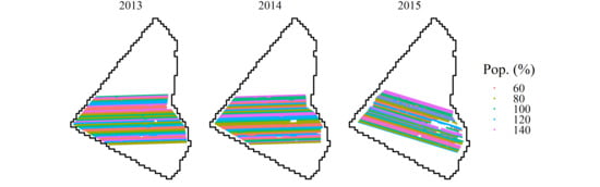
Figure 1.
Field experiment design showing long strips of fixed plant density rates across management zones.
After the plants’ emergence, the seeding rate quality was evaluated by measuring the average distance between plants. The seeding rate quality rate was determined as referred to in ISO 7256-1 standard (International Standardization Organization, 1984). The number of desired seeds by the row length or theoretical spacing between seeds (Xref) was compared to the actual spacing between them. The frequency distribution of actual spacing was assessed in terms of multiple seeds within spacing (seed spacing between 0 to 0.5 times Xref), acceptable spacing (seed spacing between 0.5 to 1.5 times Xref), and skips spacing (seed spacing larger than 1.5 times Xref).
A hydraulic motor was installed in the planter to automate rate change using vacuum seed meter distributors as well as a seeding monitor to check it. Harvesting was performed individually for each strip. The yield data were collected with the same aforementioned yield monitor (see Section 2.2). Yield data were linked to the MZs, as well as the hybrid and plant population density to perform the analysis.
2.4. Data Analysis
Initially, a descriptive statistical analysis was performed to characterize the accuracy of the density rate. Factor analyses were performed to test the factors of seeding density, hybrids, and MZ. Yield (kg ha−1) was the main variable analyzed as the response to the factors described. Additionally, regression analyses were performed to predict the response of yield to the factors. Data wrangling, all statistical analyses, and maps were produced using the R programming language and environment [].
3. Results and Discussion
3.1. Attribute Layers Analysis
Multiple seasons of maize yield maps harvested in 2009 and 2012, soybean yield map in 2013, elevation, and ECa at different depths are shown in Figure 2. The 2009 harvest of maize showed a much lower yield when compared to the 2012 harvest. The northern and southeastern regions of the field showed remarkably higher yields for the 2009 maize harvest and 2013 soybean harvest. The 2012 maize harvest, on the other hand, showed lower spatial variability of yield compared to the other two yield maps. The yield pattern seems to agree with ECa patterns, where higher ECa values are also seen in the southeastern region of the field. Elevation decreases from north to south in the field.
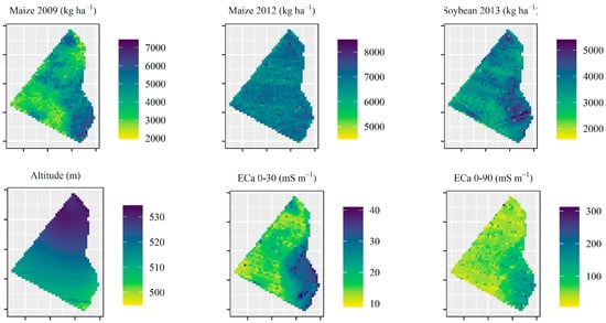
Figure 2.
Data layers are used for delimiting the management zones.
The data distribution of yield, ECa, and altitude are presented in Figure 3. Maize 2012 and Soybean 2013 show data distribution close to the normal distribution, unlike the other attributes. The ECa coefficient of variation (CV) ranged from 40.1%, for the 0 to 0.30 m depth, to 52.8%, for the 0 to 0.90 m depth, indicating substantial variability. A flatter distribution indicates higher dispersion of the collected data, while a bell-shaped curve indicates data concentrating around the mean of the data set. These results show that the variation in yield data was greater for the maize harvest in 2009 than in 2012. Low variance and high average in the 2012 maize yield map compared to 2009 probably prevent the expression of low-performance management zones, which would make it difficult to correlate the layers to management zones.
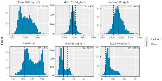
Figure 3.
Data distribution for attribute maps in the experimental field.
Because we want to use these variables to predict management zones of higher or lower performance, we can assess their correlation to yield maps from previous years. This is because regions of higher yield are usually maintained over time. The correlation analysis for the attribute maps is presented in Figure 4. As observed in Figure 2, the YM of Maize 2009 and Soybean 2013 correlated well to soil ECa. The correlation for the ECa in the two depths, shallow (0 to 0.30 m) and deep (0 to 0.90 m), with 2009 maize yield were 0.650 (confidence interval at 90%: CI90 = 0.624–0.675) and 0.651 (CI90 = 0.625–0.676), respectively, while the correlations with 2013 soybean yield were 0.470 (CI90 = 0.434–0.503) and 0.485 (CI90 = 0.450–0.518) respectively. This correlation is evident in the visual evaluation of the maps (Figure 2), in which the regions of higher yield coincide with the regions of higher ECa.
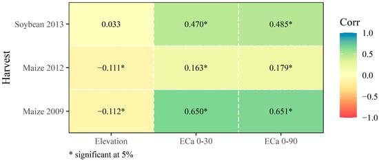
Figure 4.
Correlograms for the variables used to delimit the management zones.
A good correlation between soil ECa and crop yield has also been observed in different studies []. According to Molin et al. [] and Uribeetxebarria et al. [], ECa has been used as a proxy for soil water content, soil density and texture, organic matter content, salinity, cation exchange capacity, among other characteristics that may be difficult to measure in the field. Therefore, this layer presents a potential to be used in the planning of varied rate seeding, adjusting this for each environment. In parallel, soil fertility data may also contribute to the understanding of causes for the spatial variability evidenced by ECa.
3.2. Management Zones Definition
The strategy to implement MZs is an effective and simplifying way of managing crop variability, supporting the optimization of seeding, and application of other inputs. Moreover, when identifying the variables related to the yield variability it is possible to determine areas of high, medium, and low yield potential and thus manage them individually with specific strategies for each part of the field [].
It is generally recommended that MZs are defined considering layers that are stable over time [,]. Thus, we opted for the elevation, the yield map history, and ECa at 0 to 0.30 m, in which the greatest root system activity occurs and is better matched to monitoring by soil sampling (Figure 5). The physical–chemical properties were not used here as input for defining MZs because their stability over time has not been proved. The average yield values varied over the years and with the crop. The highest yield was reached in 2012 for maize in the high potential MZ, whereas the lowest yield was also observed for maize but in 2009 in the low potential MZ. The yield difference between the MZs was 62% in the year 2009, which means a difference of 1960 kg ha−1 more in the HMZ compared to the LMZ.
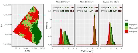
Figure 5.
Management zones based on the K-means clustering algorithm.
The spatial variability of physicochemical soil attributes was evaluated within each MZ (Table 2). The results of the analysis of variance (ANOVA) of soil attributes showed a statistically significant difference among the three MZs for almost all attributes, except for organic matter (OM), soil texture, silt, and phosphorus. The HMZ showed higher values for ECa, pH, cation exchange capacity (CEC), sand, base saturation (V), and potassium (K) than that of LMZ by 134.4%, 8.3%, 32.2%, 23.7%, 16.5%, and 36.1%, respectively. In contrast, aluminum (Al) and clay showed values 55.5% and 7.2% lower in HMZ when compared to LMZ.
Table 2.
Analysis of variance for soil attributes (0–0.20 m) in each of the management zones.
The ANOVA results show that the different MZs obtained from yield maps, altitude, and ECa were able to cluster regions with different soil textures, ECa, and nutrient concentrations. This fact can indicate that the technique used to define the MZs was rather efficient and can be used for the management of inputs and respective rates, e.g., seeding rates. The physicochemical properties of the soil may help to explain the potential performance of the different MZs. For example, Table 2 shows higher ECa in the high yield MZ, while lower pH and higher aluminum concentrations are seen in the lower yield MZ. The spatial variability of soil attributes helps in the choice of management alternatives because the crop yield can vary in the same area no matter how small the spatial variability of these attributes may be [].
3.3. Plant Distribution
The summary of the number of failures, multiple plants, acceptable spacings, and coefficient of variation are presented in Table 3 for each relative plant population in the years 2013, 2014, and 2015. The year 2013 resulted in the lowest CV among the three years of the experiment (~36%), while the year 2015 presented the highest coefficient of variation (~40%). The analysis of variance showed that the number of acceptable spacings decreases significantly (p-value < 0.01) for different relative plant populations. According to Sangoi et al. [], the losses due to poor plant distribution can reach 83 kg ha−1 for every 10% increase in the CV of the spacings between plants. According to Kolling et al. [], plants tend to compensate for the non-uniformity of plant distribution by incrementing the grain mass, which is insufficient to compensate for the overall yield losses. Therefore, the choice of relative plant population should be made carefully because higher densities decrease the seeding quality and can negatively affect the crop yield.
Table 3.
Coefficient of variation (CV) and percentage of skip spacings, acceptable spacings, and multiple plants within spacings for the five different population rates tested in 2013, 2014, and 2015.
3.4. Yield Response as a Function of Seeding Density and Management Zones
The relationship between yield and the relative population seeding for each hybrid in each year of study is presented in Figure 6. The increase of relative population was proportional to the increase of yield in 2013 and 2015, i.e., there was an increase in yield with the increase of plant population. In 2014, however, there was no increase of yield with the increase of population from 120% to 140%, and there was even a decrease of yield for the hybrid AG 9030.
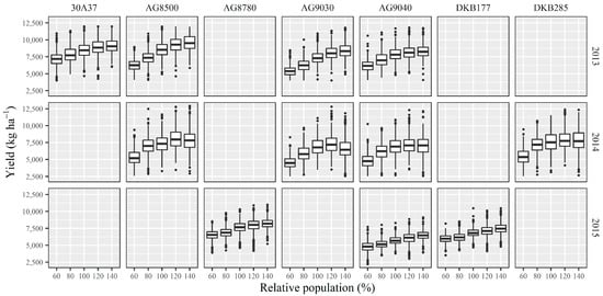
Figure 6.
Relationship between yield and relative seeding rate for maize in the experimentation period.
The second crop harvest is characterized by greater climatic risk when compared to the first harvest, especially risks of reduced yield as a result of water deficit. The harvest of 2015 showed remarkably lower yields when compared to 2013 and 2014. In the years 2013 and 2014, the rainfall rates were generally close to or above the historical average of the last 20 years (Figure 7). In 2015, however, rainfall rates were below the historical average, especially in March, when the crop was in the initial stage of development, and in June, when the crop was in the R2 and R3 reproductive stages. Thus, water stress may have been one of the factors that affected the productivity of the crop in 2015. In contrast, the good availability of water and the absence of other bad weather such as frost and strong winds provided good conditions for the development of maize as a secondary crop in the years 2013 and 2014.
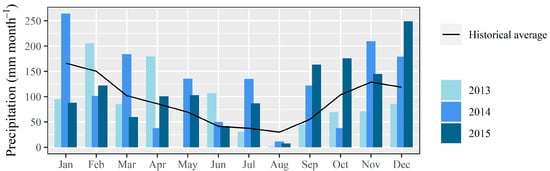
Figure 7.
Monthly rainfall for the years 2013, 2014, 2015, and the historical average for the region of Maracajú, MS, Brazil. Data source: Automatic weather station A731-INMET, 2020.
The effects of plant population variation within each MZ are presented in Figure 8. As expected, the yields were higher within the high-performance MZ than that of the medium and low-performance MZ in all three years of the experiment. The effect of the MZs became more evident as the relative plant population increased. This trend occurs in all three years of the experiment. The low and medium yield MZ did not show an increase in yields for the increase in relative population from 120% to 140%, reaching a plateau. In contrast, the high-yielding MZ had an increase of yield with the increase in relative plant population, reaching the highest yield values among the three MZs. This means that high-performance MZ can further increase yield at higher seeding densities, whereas the low- and medium-performance MZs will limit crop productivity.
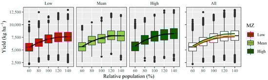
Figure 8.
Relationship between maize yield and its relative population in the second crop harvest for each of the three management zones.
The variation in effective population within each MZ over the experiment years is shown in Figure 9. The year 2013 showed the greatest difference between yields within each MZ. In the years in which the mean yield of the plot was higher, the difference between the MZs was accentuated. As expected, in all years there was a difference in maize yield between the high and low potential MZs, where the high potential MZ presented the highest yields.
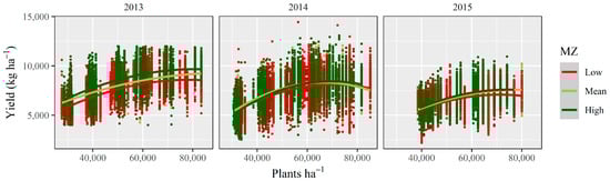
Figure 9.
Population effect on yield for the different management zones for the second crop harvest (maize) of the years 2013, 2014, and 2015.
As some condition restricts yield, the difference between the MZ is smoothed, especially at lower populations, as in 2014 and 2015. This restriction in productivity for 2015 can be explained by the damage caused by wild pigs that destroyed part of the experiment and affected the plant stand. This increased the number of skips in the seeding lines. Moreover, when the environment is more restrictive to yield, the population range that maximizes yield is narrower. Therefore, the farmer needs to be more assertive about the number of plants per area to obtain a satisfactory yield. The yield within each MZ and the descriptive statistics of the data are shown in Figure 10.
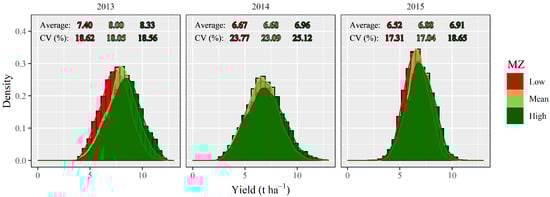
Figure 10.
Maize yield for the management zones in the second crop harvest of 2013, 2014, and 2015.
The yield difference between high and low potential MZ was 930 kg ha−1, 290 kg ha−1, and 390 kg ha−1 for the years 2013, 2014, and 2015, respectively. The highest coefficient of variation among yield values occurred in 2014. The results showed that the high potential MZ always produced more than the low potential MZ. The maximum yields were reached between populations of 70,000 plants ha−1 and 80,000 plants ha−1 (Figure 9), with a decreasing yield with an increased population above this limit. In other words, the plant population range where the maximum yield was reached is at least 27% above the 55,000 plants ha−1 density used by the farmers in the region where the study was carried out. However, it is fundamental to consider that there is the possibility of lower populations performing better in more restrictive years, especially concerning the frequency and total rainfall.
These results are different from those presented by Hörbe et al. [], in southern Brazil. It is important to point out that in this country region, only the first crop occurs. Therefore, maize yields as a principal crop, i.e., grown in summer, tend to result in higher yields. The authors managed to reduce the seeding density by up to 29% in relation to the standard population used in the southern region of Brazil (70,000 plants ha−1). The yield also increased by approximately 1900 kg ha−1 in the low-performance MZ. On the other hand, the tendency for high potential MZs was similar in both studies, i.e., the increase in population generated an increase in yield.
Different clustering algorithms have also been used to delineate management zones. For example, Gavioli et al. [] tested 20 clustering algorithms and similar field attributes, like elevation, yield maps, and soil physical properties. Here, we did not use physical attributes, however, those have been shown to correlate well to ECa []. Gavioli et al. [] showed that the management zones delineated using attributes that are stable over time were also able to segregate zones with different chemical properties, as also observed here (Table 2). Besides, management zones can also be used for different purposes. Barman et al. [] defined management zones to improve the efficacy of input recommendations. The authors showed how management zones can be useful not only to save resources but for balanced fertilization and sustainable restoration of sodic lands. Cid-Garcia and Ibarra-Rojas [] also showed that management zones can increase the profit for multiple crops.
The interference of chemical variables and soil texture in the yield of each management zone and year is shown in Figure 11 and Figure 12. Figure 11 presents the scatterplots between the management zone attributes and yield, whereas Figure 12 presents a principal component analysis (PCA) performed considering the main soil fertility parameters. The first two principal components account for approximately 63% of the total data variability (Figure 12).
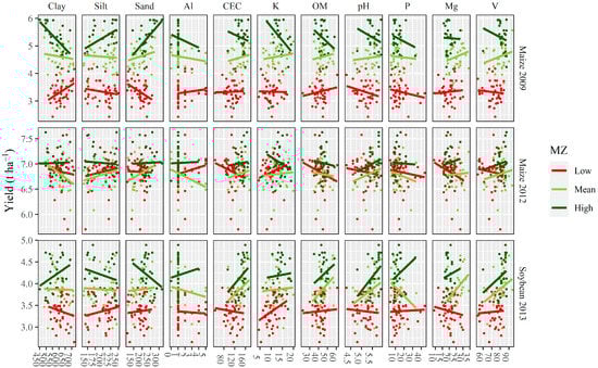
Figure 11.
Chemical variables and soil texture in relation to productivity for each management zone and year.
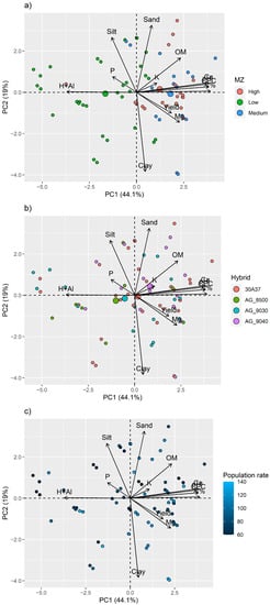
Figure 12.
Principal component analysis (PCA) of soil attributes and maize yield in the first year of the experiment (2013) for classes of management zones (a), hybrids (b), and population rate (c).
The biplot for the two first components suggests that the yield is related directly to Mg content. The variance in CEC, V, pH, and Ca attributes can be explained mainly by PC1. The contribution of these attributes is similar, with their partial overlapping along the positive direction of this component. On the other hand, variance in clay can be explained mainly by the negative direction of PC2. Moreover, the yield varies in the positive direction of PC1 and negative in PC2, with similar contributions from both components, suggesting that all these soil parameters contributed most to the variance of yield when compared to other soil parameters.
For most samples, the explained variance of most of the evaluated parameters occurred in the high and medium potential management zones (Figure 12a), and with plant population above the recommended sowing rate (>100%, Figure 12c), except for H + Al, P, and silt. Furthermore, there was no clear effect of the explained variance of the parameters evaluated as a function of the hybrid (Figure 12b).
4. Conclusions
This study assessed the performance of seven maize hybrids and five seeding rates under different management zones. The management zones were defined using a clustering algorithm and layers based on yield maps from previous years, elevation, and soil apparent electric conductivity. The zones were then classified as low, medium, and high yield potential based on the yield maps from previous years. The soil was sampled using a regular grid to investigate the soil physical and chemical properties that could play a key role within each management zone.
In general, yield increased and, in some cases, reached stability for higher seeding rates. For low seeding rates, there was little difference between yields obtained for each management zone. In contrast, under higher seeding rates, the high potential management zone resulted in significantly higher yields.
The statistical analyses showed that several soil attributes are responsible for governing a zone with lower or higher potential yield. For example, lower pH and higher aluminum concentrations were related to lower grain yields. On the other hand, higher organic matter content, cation exchange capacity, base saturation, potassium concentration, and soil apparent electric conductivity were related to higher grain yields.
This study showed that the management of different seeding rates in different zones, in addition to being a low-cost technique, can result in reduced input application costs and optimize the yield according to the site-specific potential of the field. Future studies should focus on evaluating cause-and-effect relationships with soil and climate parameters over the years, and their effect on yield and plant population. In addition, they should consider economics and environmental indicators for developing optimization algorithms to support plant density decisions from more holistic perspectives.
Author Contributions
Conceptualization, J.P.M. and A.A.A.; methodology, J.P.M., A.A.A., H.C.B. and L.d.P.C.; software, H.C.B. and L.d.P.C.; formal analysis, J.P.M., A.A.A., H.C.B. and L.d.P.C.; investigation, J.P.M., A.A.A., H.C.B. and L.d.P.C.; writing—original draft preparation, J.P.M., A.A.A., H.C.B. and L.d.P.C.; writing—review and editing, J.P.M., H.C.B. and L.d.P.C.; visualization, H.C.B. and L.d.P.C.; supervision, J.P.M. All authors have read and agreed to the published version of the manuscript.
Funding
The Coordination for the Improvement of Higher Education Personnel (Coordenação de Aperfeiçoamento de Pessoal de Nível Superior—CAPES) provided the doctoral scholarship to H.C.B. (Finance Code 001) and the National Council for Scientific and Technological Development (Conselho Nacional de Desenvolvimento Científico e Tecnológico—CNPq) provided the doctoral scholarship to A.A.A.
Institutional Review Board Statement
Not applicable.
Informed Consent Statement
Not applicable.
Data Availability Statement
The data presented in this study are available on request from the corresponding author.
Conflicts of Interest
The authors declare no conflict of interest.
References
- Sher, A.; Khan, A.; Cai, L.J.; Irfan Ahmad, M.; Asharf, U.; Jamoro, S.A. Response of Maize Grown Under High Plant Density; Performance, Issues and Management—A Critical Review. Adv. Crop Sci. Technol. 2017, 5, 275. [Google Scholar] [CrossRef] [Green Version]
- Gavioli, A.; de Souza, E.G.; Bazzi, C.L.; Schenatto, K.; Betzek, N.M. Identification of management zones in precision agriculture: An evaluation of alternative cluster analysis methods. Biosyst. Eng. 2019, 181, 86–102. [Google Scholar] [CrossRef]
- Molin, J.P.; Bazame, H.C.; Maldaner, L.; Corredo, L.d.P.; Martello, M.; Canata, T.F. Precision agriculture and the digital contributions for site-specific management of the fields. Rev. CIÊNCIA AGRONÔMICA 2020, 51, 1–10. [Google Scholar] [CrossRef]
- Munnaf, M.A.; Haesaert, G.; Van Meirvenne, M.; Mouazen, A.M. Site-specific seeding using multi-sensor and data fusion techniques: A review. In Advances in Agronomy; Academic Press Inc.: Cambridge, MA, USA, 2020; Volume 161, pp. 241–323. ISBN 9780128207659. [Google Scholar]
- da Silva, E.E.; Baio, F.H.R.; Teodoro, L.P.R.; Campos, C.N.S.; Plaster, O.B.; Teodoro, P.E. Variable-rate seeding in soybean according to soil attributes related to grain yield. Precis. Agric. 2021, 1–17. [Google Scholar] [CrossRef]
- Licht, M.A.; Lenssen, A.W.; Elmore, R.W. Corn (Zea mays L.) seeding rate optimization in Iowa, USA. Precis. Agric. 2017, 18, 452–469. [Google Scholar] [CrossRef] [Green Version]
- Coronel, E.G.; Alesso, C.A.; Bollero, G.A.; Armstrong, K.L.; Martin, N.F. Field-specific yield response to variable seeding depth of corn in the Midwest. Agrosystems Geosci. Environ. 2020, 3, e20034. [Google Scholar] [CrossRef]
- Chen, S.; Du, T.; Wang, S.; Parsons, D.; Wu, D.; Guo, X.; Li, D. Quantifying the effects of spatial-temporal variability of soil properties on crop growth in management zones within an irrigated maize field in Northwest China. Agric. Water Manag. 2021, 244, 106535. [Google Scholar] [CrossRef]
- Rodrigues, M.S.; Corá, J.E. Management zones using fuzzy clustering based on spatial-temporal variability of soil and corn yield. Eng. Agric. 2015, 35, 470–483. [Google Scholar] [CrossRef] [Green Version]
- Oldoni, H.; Silva Terra, V.S.; Timm, L.C.; Júnior, C.R.; Monteiro, A.B. Delineation of management zones in a peach orchard using multivariate and geostatistical analyses. Soil Tillage Res. 2019, 191, 1–10. [Google Scholar] [CrossRef]
- Breunig, F.M.; Galvão, L.S.; Dalagnol, R.; Santi, A.L.; Della Flora, D.P.; Chen, S. Assessing the effect of spatial resolution on the delineation of management zones for smallholder farming in southern Brazil. Remote Sens. Appl. Soc. Environ. 2020, 19, 100325. [Google Scholar] [CrossRef]
- Breunig, F.M.; Galvão, L.S.; Dalagnol, R.; Dauve, C.E.; Parraga, A.; Santi, A.L.; Della Flora, D.P.; Chen, S. Delineation of management zones in agricultural fields using cover–crop biomass estimates from PlanetScope data. Int. J. Appl. Earth Obs. Geoinf. 2020, 85, 102004. [Google Scholar] [CrossRef]
- Cordero, E.; Longchamps, L.; Khosla, R.; Sacco, D. Joint measurements of NDVI and crop production data-set related to combination of management zones delineation and nitrogen fertilisation levels. Data Br. 2020, 28, 104968. [Google Scholar] [CrossRef]
- Arshad, M.; Li, N.; Zhao, D.; Sefton, M.; Triantafilis, J. Comparing management zone maps to address infertility and sodicity in sugarcane fields. Soil Tillage Res. 2019, 193, 122–132. [Google Scholar] [CrossRef]
- Méndez-Vázquez, L.J.; Lira-Noriega, A.; Lasa-Covarrubias, R.; Cerdeira-Estrada, S. Delineation of site-specific management zones for pest control purposes: Exploring precision agriculture and species distribution modeling approaches. Comput. Electron. Agric. 2019, 167, 105101. [Google Scholar] [CrossRef]
- Kayad, A.; Sozzi, M.; Gatto, S.; Whelan, B.; Sartori, L.; Marinello, F. Ten years of corn yield dynamics at field scale under digital agriculture solutions: A case study from North Italy. Comput. Electron. Agric. 2021, 185, 106126. [Google Scholar] [CrossRef]
- Miao, Y.; Mulla, D.J.; Robert, P.C. An integrated approach to site-specific management zone delineation. Front. Agric. Sci. Eng. 2018, 5, 432–441. [Google Scholar] [CrossRef] [Green Version]
- Paccioretti, P.; Córdoba, M.; Balzarini, M. FastMapping: Software to create field maps and identify management zones in precision agriculture. Comput. Electron. Agric. 2020, 175, 105556. [Google Scholar] [CrossRef]
- Hörbe, T.A.N.; Amado, T.J.C.; Ferreira, A.O.; Alba, P.J. Optimization of corn plant population according to management zones in Southern Brazil. Precis. Agric. 2013, 14, 450–465. [Google Scholar] [CrossRef]
- Li, J.; Xie, R.Z.; Wang, K.R.; Ming, B.; Guo, Y.Q.; Zhang, G.Q.; Li, S.K. Variations in maize dry matter, harvest index, and grain yield with plant density. Agron. J. 2015, 107, 829–834. [Google Scholar] [CrossRef]
- Schenatto, K.; de Souza, E.G.; Bazzi, C.L.; Gavioli, A.; Betzek, N.M.; Beneduzzi, H.M. Normalization of data for delineating management zones. Comput. Electron. Agric. 2017, 143, 238–248. [Google Scholar] [CrossRef]
- Spekken, M.; Anselmi, A.A.; Molin, J.P. A simple method for filtering spatial data. In Proceedings of the Precision Agriculture 2013, Proceedings of the 9th European Conference on Precision Agriculture, ECPA 2013; Wageningen Academic Publishers: Wageningen, The Netherlands, 2013; pp. 259–266. [Google Scholar]
- R Core Team. A Language and Environment for Statistical Computing; R Core Team: Vienna, Austria, 2021. [Google Scholar]
- Wang, X.X.; Liu, S.; Zhang, S.; Li, H.; Maimaitiaili, B.; Feng, G.; Rengel, Z. Localized ammonium and phosphorus fertilization can improve cotton lint yield by decreasing rhizosphere soil pH and salinity. F. Crop. Res. 2018, 217, 75–81. [Google Scholar] [CrossRef]
- Molin, J.P.; Rabello, L.M. Estudo sobre a mensuração da condutividade elétrica do solo. Eng. Agrícola 2011, 31, 90–101. [Google Scholar] [CrossRef]
- Uribeetxebarria, A.; Arnó, J.; Escolà, A.; Martínez-Casasnovas, J.A. Apparent electrical conductivity and multivariate analysis of soil properties to assess soil constraints in orchards affected by previous parcelling. Geoderma 2018, 319, 185–193. [Google Scholar] [CrossRef] [Green Version]
- Albornoz, V.M.; Ñanco, L.J.; Sáez, J.L. Delineating robust rectangular management zones based on column generation algorithm. Comput. Electron. Agric. 2019, 161, 194–201. [Google Scholar] [CrossRef]
- Umbelino, A.D.S.; De Oliveira, D.G.; Martins, M.P.D.O.; Reis, E.F. Dos Definições de zona de manejo para soja de alta produtividade. Rev. Ciências Agrárias 2018, 41, 674–682. [Google Scholar] [CrossRef]
- Sangoi, L.; Schmitt, A.; Vieira, J.; José Picoli, G.J.; Arruda Souza, C.; Trezzi Casa, R.; Eduardo Schenatto, D.; Giordani, W.; Majolo Boniatti, C.; Cardoso Machado, G.; et al. Revista Brasileira de Milho e Sorgo; Associação Brasileira de Milho e Sorgo: Sete Lagoas, Brazil, 2013; ISSN 1676-689X. [Google Scholar]
- Kolling, D.F.; Sangoi, L.; de Souza, C.A.; Schenatto, D.E.; Giordani, W.; Boniatti, C.M. Tratamento de sementes com bioestimulante ao milho submetido a diferentes variabilidades na distribuição espacial das plantas. Cienc. Rural 2016, 46, 248–253. [Google Scholar] [CrossRef] [Green Version]
- Barman, A.; Sheoran, P.; Yadav, R.K.; Abhishek, R.; Sharma, R.; Prajapat, K.; Singh, R.K.; Kumar, S. Soil spatial variability characterization: Delineating index-based management zones in salt-affected agroecosystem of India. J. Environ. Manag. 2021, 296, 113243. [Google Scholar] [CrossRef]
- Cid-Garcia, N.M.; Ibarra-Rojas, O.J. An integrated approach for the rectangular delineation of management zones and the crop planning problems. Comput. Electron. Agric. 2019, 164, 104925. [Google Scholar] [CrossRef]
Publisher’s Note: MDPI stays neutral with regard to jurisdictional claims in published maps and institutional affiliations. |
© 2021 by the authors. Licensee MDPI, Basel, Switzerland. This article is an open access article distributed under the terms and conditions of the Creative Commons Attribution (CC BY) license (https://creativecommons.org/licenses/by/4.0/).