Application of Three Deep Machine-Learning Algorithms in a Construction Assessment Model of Farmland Quality at the County Scale: Case Study of Xiangzhou, Hubei Province, China

Abstract

Constructing a scientific and quantitative quality-assessment model for farmland is important for understanding farmland quality, and can provide a theoretical basis and technical support for formulating rational and effective management policies and realizing the sustainable use of farmland resources. To more accurately reflect the systematic, complex, and differential characteristics of farmland quality, this study aimed to explore an intelligent farmland quality-assessment method that avoids the subjectivity of determining indicator weights while improving assessment accuracy. Taking Xiangzhou in Hubei Province, China, as the study area, 14 indicators were selected from four dimensions—terrain, soil conditions, socioeconomics, and ecological environment—to build a comprehensive assessment index system for farmland quality applicable to the region. A total of 1590 representative samples in Xiangzhou were selected, of which 1110 were used as training samples, 320 as test samples, and 160 as validation samples. Three models of entropy weight (EW), backpropagation neural network (BPNN), and random forest (RF) were selected for training, and the assessment results of farmland quality were output through simulations to compare their assessment accuracy and analyze the distribution pattern of farmland quality grades in Xiangzhou in 2018. The results showed the following: (1) The RF model for farmland quality assessment required fewer parameters, and could simulate the complex relationships between indicators more accurately and analyze each indicator’s contribution to farmland quality scientifically. (2) In terms of the average quality index of farmland, RF > BPNN > EW. The spatial patterns of the quality index from RF and BPNN were similar, and both were significantly different from EW. (3) In terms of the assessment results and precision characterization indicators, the assessment results of RF were more in line with realities of natural and socioeconomic development, with higher applicability and reliability. (4) Compared to BPNN and EW, RF had a higher data mining ability and training accuracy, and its assessment result was the best. The coefficient of determination (R²) was 0.8145, the mean absolute error (MAE) was 0.009, and the mean squared error (MSE) was 0.012. (5) The overall quality of farmland in Xiangzhou was higher, with a larger area of second- and third-grade farmland, accounting for 54.63%, and the grade basically conformed to the trend of positive distribution, showing an obvious pattern of geographical distribution, with overall high performance in the north-central part and low in the south. The distribution of farmland quality grades also varied widely among regions. This showed that RF was more suitable for the quality assessment of farmland with complex nonlinear characteristics. This study enriches and improves the index system and methodological research of farmland quality assessment at the county scale, and provides a basis for achieving a threefold production pattern of farmland quantity, quality, and ecology in Xiangzhou, while also serving as a reference for similar regions and countries.

1. Introduction

Farmland is an important natural resource for people to carry out agricultural production, and it plays an important role in ensuring food security, promoting sustainable economic development, and maintaining social harmony and stability [1,2,3]. However, since the reform and opening up of China, which was accompanied by accelerated urbanization, the amount of farmland area has decreased sharply, especially high-quality farmland around the cities, which has been occupied to a larger extent, creating certain challenges to food security. In order to strictly adhere to the red line of 120 million hectares of farmland, the Chinese government has formulated a very stringent farmland protection system. In the past 10 years, the area of farmland in China has increased to some extent, but the quality has decreased overall, with only 27.3% corresponding to high-quality farmland [4]. In addition, the input of new technologies and varieties has brought hidden security risks—such as pollution—to farmland, which seriously threatens sustainable socioeconomic development and the ecological environment [5]. Therefore, actively carrying out studies on farmland quality assessment; effectively improving and protecting farmland quality; implementing a threefold production pattern of farmland quantity, quality, and ecology; and firmly guarding the red line of farmland are reliable ways to achieve coordinated and sustainable economic and social development and address food security.

The quality of farmland refers to the status and condition of the land [6]. Farmland quality has extended from a single dimension of basic land fertility to a comprehensive quality involving suitability, production potential, soil environmental quality, and sustainability [7,8,9]. Scholars in other countries mainly study the temporal and spatial evolution and sustainable use of farmland, while those in China are more concerned with assessing farmland quality and its connection to food production capacity [10]. At present, there is no standard definition of farmland quality. It is generally accepted that farmland quality is the mixed result of natural, social, economic, and technological progress [11], including four aspects: soil, spatial, management, and ecological quality [12]. The assessment of farmland is a quantitative measure of its state or the extent to which it meets functional needs [13].

Traditional farmland quality assessment mainly considers the natural production potential of land, selects natural factors to construct an index system, and evaluates the suitability of farmland [14,15]. In recent years, environmental factors such as social development, economic level, and utilization patterns have received attention in farmland quality assessment, and the focus has shifted to considering many factors, such as natural, ecological, social, and economic factors [16,17,18]. In the assessment of farmland quality, different methods are chosen due to differences in the objectives and selection of indicators. The increasing research and application of “3S” technology which refers to remote sensing (RS), geography information systems (GIS), and global positioning systems (GPS), computer technology, and mathematical models has led to the development of more methods for farmland quality assessment, ranging from simple qualitative description to quantitative analysis. However, no matter which method is used, the selection of assessment indicators, classification criteria of indicators, and determination of indicator weights will affect the accuracy of assessment. Therefore, constructing a reasonable index system and exploring effective methods have become important elements of the current research on farmland quality assessment.

Currently, the main methods commonly used for farmland quality assessment are entropy weight (EW) [19], fuzzy assessment [20], analytic hierarchy process (AHP) [21], grey correlation analysis [22], and geostatistical methods [23]. EW assigns objective weights based on the physical characteristics of the data, but does not introduce human cognitive judgment of the assessment indicators [19]. The AHP is more subjective, and it is difficult to balance the sensitivity of indicator weights [21]. Fuzzy assessment, grey correlation analysis, and geostatistical methods are less stable in handling high-dimensional data, and have difficulties in drilling down into nonlinear information [24]. In recent years, the use of artificial intelligence algorithms has become a hot method for constructing models for farmland quality assessment, among which artificial neural network and support vector machine (SVM) are typical representatives [25]. Qie et al. [26], Gao [27], and Shekofteh et al. [28] applied a self-organizing neural network, a backpropagation neural network (BPNN), and a genetic algorithm–BP neural network, respectively, to evaluate farmland quality. Gayen et al. [29] used support vector machine to evaluate the sensitivity of farmland soil erosion. Lai et al. [30] used rough sets and support vector machine to evaluate the quality of high-standard farmland.

The artificial neural network has strong robustness, memory ability, nonlinear mapping ability, and self-learning ability. It is capable of digging deep into the intricate relationships between indicators and autonomously constructing a mathematical model between the assessment object and the indicators. However, there are shortcomings, such as overfitting, large generalization errors, and difficulty in determining indicator weight [31]. Compared to the artificial neural network, the support vector machine has strong adaptive and generalization capability for high-dimensional and nonlinear data [32]. It can convert assessment problems into convex optimization problems with equal value, such that the weight of indicators can be determined according to the data distribution [33]. It overcomes the problem of local overfitting, but also suffers from problems such as difficult sample partitioning, subjective parameter selection, and overlearning [34]. Thus, how to effectively unify multisource environmental variables into the same assessment unit remains a key and difficult issue in the assessment of farmland quality.

Random forest (RF) is a machine-learning algorithm for constructing multiple decision trees for combinatorial classification based on a random resampling technique (bootstrap) and random node splitting technique, and has strong anti-noise and model generalization abilities [35]. RF can achieve a higher prediction rate with optimal parameters and minimum error based on smaller training samples [36]. It can evaluate the importance of indicators during the training process, and thus solve the problem of overfitting indicators within a nonlinear complex system [37].

Farmland quality is a complicated system combining natural, socioeconomic, and ecological factors that requires superior intelligent algorithms to overcome the challenges of nonlinearity, high dimensionality, and missing values. At the same time, RF, as a nonparametric decision tree model, combines all the advantages of previous assessment methods, and has the advantage of dealing with the nonlinear relationships and weight dynamics of high-dimensional data. High prediction accuracy is maintained even when training samples have noise and are missing values. Thus, it is feasible to evaluate farmland quality using a random forest model [38]. Khamoshi et al. [39] used random forest for mapping soil and evaluating the suitability of farmland. Bhowmik et al. [40] evaluated the quality of soil environment based on random forest. Chen et al. [41] used random forest to measure the importance of assessment indicators and construct an assessment index system for farmland capacity enhancement potential. Lin et al. [42] used random forest and correlation analyses to select indicators of quality farmland and determine their weights.

Taking Xiangzhou of Hubei Province in China as an example, an assessment index system applicable to this region was constructed, and three models of entropy weight (EW), backpropagation neural network (BPNN), and random forest (RF) were selected for farmland quality assessment to avoid the subjectivity of determining index weights, and to compare the assessment accuracy of the three methods to verify the reliability and superiority of the RF model in this study. This study aimed to explore new ways to evaluate farmland quality, expand the methodology of farmland quality assessment, and improve the accuracy of assessment, in addition to serving as a reference for similar studies.

2. Materials and Methods

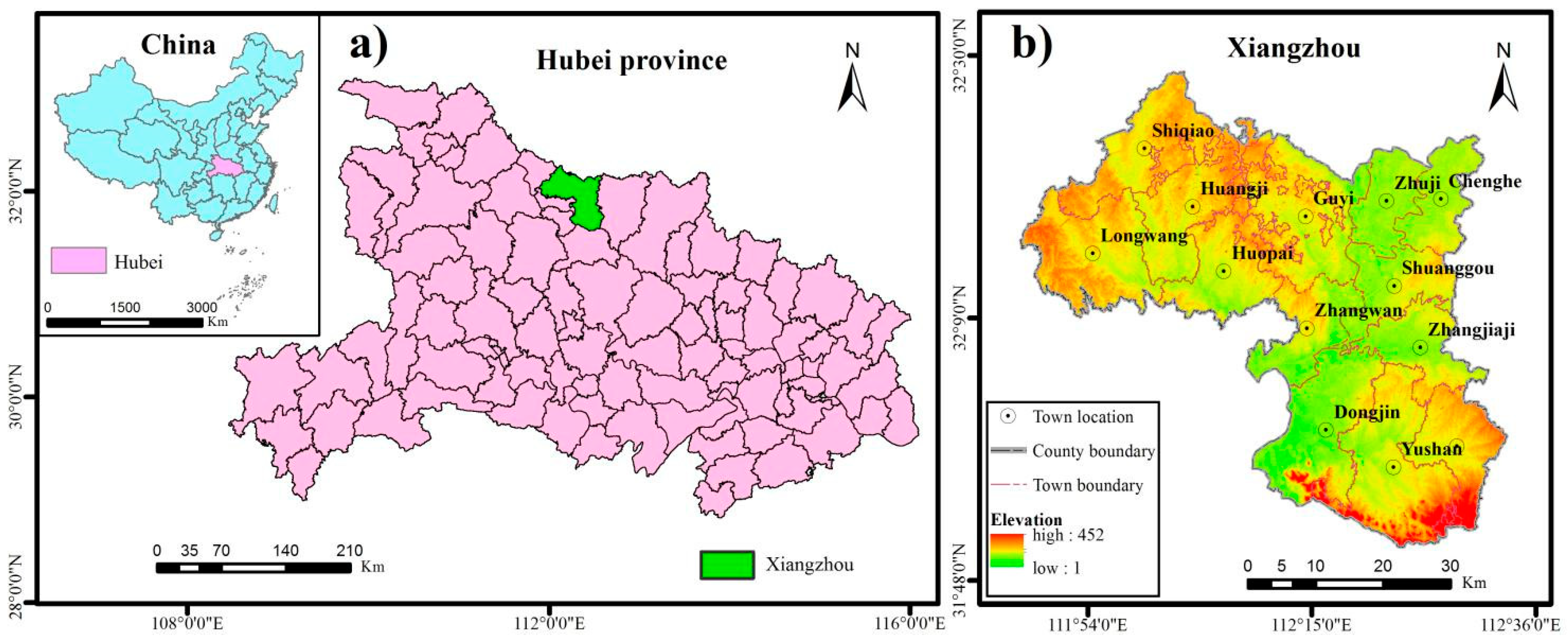
2.1. Study Area

Xiangzhou is a county-level city in the northwestern part of Hubei Province in China (Figure 1a) near the middle stream of the Han River, located between 111°44′–112°23′ E and 31°46–32°28′ N. This county is a hilly and mountainous area surrounded by low mountains, with basins and plains in the middle (Figure 1b). The landscape pattern is around 70% hillocks, 10% mountains, and 20% plains. Xiangzhou belongs to a subtropical humid monsoon continental climate zone that is affected by alternating cold and warm air. The county has four distinct seasons, with the same hot and rainy seasons, moderate precipitation, and an average annual temperature of 15.3–15.8 °C. As of 2018, the total area of arable land in Xiangzhou was 165,257 ha, accounting for 66.98%. Xiangzhou has excellent natural and ecological conditions and strong food-production capacity in Hubei Province, with wheat, rice, and corn as the main grain crops [43]. The total grain output was 1,172,800 tons in 2018. However, in recent years, with the acceleration of urbanization, a large amount of high-quality farmland around towns has been occupied, and frequent human disturbances have caused some harm to the farmland quality and soil ecology [44]. Therefore, it is of great importance to scientifically evaluate the quality of farmland toward improving food-production capacity and security. The natural environment and socioeconomic conditions of Xiangzhou are representative of the assessment of farmland quality and, thus, this area was selected as the study area.

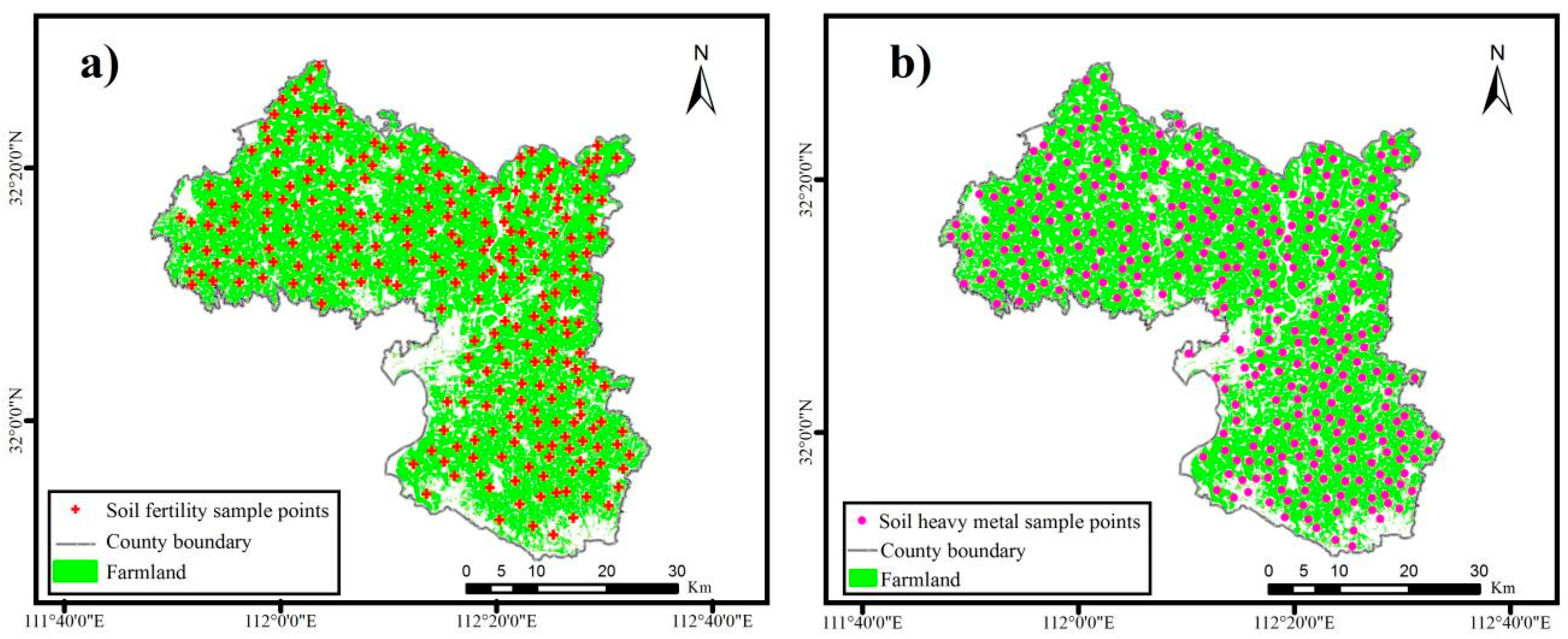
2.1.1. Data Collection

Considering the reliability and accessibility of data, the multisource environmental data involved in this study mainly included map data, soil sampling data, and socioeconomic statistics. The Land Use Change Survey Database of Xiangzhou in 2018 (1:10,000) was used to obtain administrative maps, farmland patches, rural settlements, rural roads, highways, ditches, and rivers. The Survey and Assessment of the Farmland Quality Grade of Xiangzhou in 2018 (1:10,000) (containing 255 soil sampling points) was used to extract the soil fertility index. The Farmland Soil Environmental Quality Category Classification Database of Xiangzhou in 2018 (1:10,000) (containing 326 soil heavy-metal sampling points) was used to obtain the soil cleanliness index. The slope was extracted using a 30 m resolution digital elevation model (DEM) from the Resource and Environment Science and Data Center (http://www.resdc.cn). The 2018 Statistical Yearbook and related agricultural statistics in Xiangzhou were used to extract socioeconomic and other statistical data.

2.1.2. Data Processing

(1)

Soil index data processing

Following the principles of comprehensiveness, representativeness, objectivity, equilibrium, comparability, and accessibility [5], 255 soil sampling points (Figure 2a) were selected at the center of representative plots in the study area and sampled before soil fertilization following the autumn harvest of 2018 crops, using a handheld GPS for coordinate positioning, to collect the surface layer of 0–20 cm of cultivated soil. Each soil sample was mixed in a star or S shape according to the size of the plot, and 1 kg was collected in a bag for analysis. More than 30 items of information related to the sampling point and its surrounding environment were recorded, such as topographic site, surface soil texture, texture configuration, tillage-layer thickness, barrier factors, biodiversity, reticulation of agricultural land and forestry, and other soil properties, among which tillage-layer thickness was obtained by field measurement, and biodiversity was obtained by calculating the percentage of earthworms at the sample point.

Soil characteristics such as pH, moisture, available phosphorus, available potassium, and organic matter were obtained by soil sample assay analysis. In addition, there were 326 heavy-metal sampling points (Figure 2b) in the farmland of the study area, and the contents of five soil polluting elements—Pb, Cd, Cr, Hg, and As—were obtained by sample assay analysis. On this basis, the Kriging interpolation value with less error was selected by cross-validation comparison of inverse distance weight and values from Kriging, and polynomial methods. Kriging optimal interpolation was performed on the selected index data in this study according to the optimal semi-covariance function model [45]. Regarding the accuracy of test results after interpolation of soil pH, the mean absolute error (MAE) was 0.056, the root mean square error (RMSE) was 0.078, and the agreement coefficient (AC) was 0.913, indicating that the interpolation effect was ideal. The remaining indicators were validated in a similar way, and spatial distribution maps of each indicator were generated after test correction.

(2)

Socioeconomic index data processing

Using ArcGIS 10.2 software developed by the Environmental Systems Research Institute in RedLands, California, USA, we obtained socioeconomic indicators of farmland quality, such as farming distance, ease of farming, traffic accessibility, drainage capacity, and irrigation capacity, using neighborhood analysis tools. Farming distance was obtained by calculating the distance from the farmland patch to the rural settlement; ease of farming was obtained by calculating the distance from the farmland patch to the rural road; traffic accessibility was obtained by calculating the distance from the farmland patch to the highway; drainage capacity was obtained by calculating the distance from the farmland patch to the ditch; and irrigation capacity was obtained by calculating the distance from the farmland patch to the river.

Based on the Land Use Change Survey database of Xiangzhou in 2018, the arable land patches were extracted as assessment units, and there were 16,072 found. Meanwhile, ArcGIS 10.2 was used to realize the projection transformation and vectorization of each indicator.

2.2. Methods

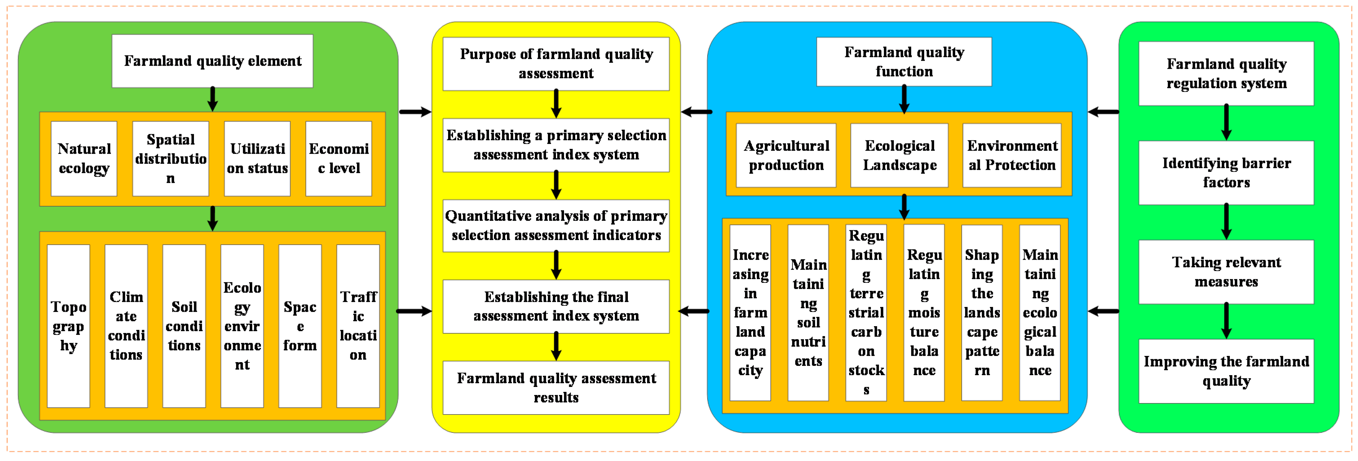
2.2.1. Building a Comprehensive Index System for Farmland Quality Assessment

(1)

Preliminary Selection of Indicators

Farmland is a complex system formed by the interaction of various factors, such as climate, topography, physical and chemical properties of the soil, and human activities [3], and its quality is influenced by multiple factors. Therefore, in the selection of indicators, the influence of each factor on farmland quality should be considered comprehensively, and the dominant factor should be selected as the assessment indicator. In terms of scale effect, the selection of assessment indicators should be compatible with the assessment spatial scale. In terms of demand function, the intrinsic attributes reflected by farmland quality should serve not only as the economic value function of agricultural production, but also as the ecological service function, as an important part of a terrestrial ecosystem; for example, controlling soil nutrient loss, regulating carbon storage capacity, storing and regulating water balance capacity, shaping landscape patterns, and maintaining ecological balance [46]. In addition, the fundamental purpose of the assessment is to provide a scientific basis for carrying out quality regulation based on an accurate grasp of farmland quality and obstacle factors, so the selection of assessment indicators also needs to identify obstacles to better serve farmland quality regulation.

Based on the above theoretical analysis, the framework of a farmland quality assessment index system was established based on element–function–regulation in this study (Figure 3), which shows the connotation of farmland quality at different levels. In this framework, the term “element” refers to influencing factors, reflecting the influence of the coupling of factors on farmland quality at a certain spatial scale. Soil conditions are the basis of high agricultural yield, and are the most important factors affecting farmland quality, giving priority to soil pH, available phosphorus, available potassium, organic matter, and other indicators reflecting the fertility [47]. The term “function” refers to the functional role of farmland quality in agricultural production, ecological landscape, and environmental protection, reflecting the intrinsic needs of human exploitation and ecological processes, with an emphasis on indicators reflecting the sustainable use of farmland, such as biodiversity and soil environmental quality [48,49]. The term “regulation” refers to the implementation of appropriate regulation measures to enhance farmland quality. Topography, field drainage and irrigation facilities, and transportation locations are obstacle factors that limit the improvement of farmland quality [50] and need to be regulated through soil management, so these factors should also be considered in the assessment of farmland quality.

In this study, a preliminary assessment indicator system of farmland quality consisting of 19 indicators was constructed from four aspects—terrain, soil conditions, socioeconomics, and ecological environment (

Table 1. System of indicators for evaluating the quality of farmland.

Normative Layer	Indicator Layer	Basis of Calculation	Explanation
Terrain	Slope	Based on digital elevation model (DEM) calculations	Reservation
	Topographic site (TS)	Based on sample point assay data from survey and assessment of farmland quality grade of Xiangzhou in 2018	Reservation
Soil conditions	Surface soil texture (SST)		Reservation
	Texture configuration (TC)		Deletion
	Tillage layer thickness (TLT)		Reservation
	Barrier factor (BF)		Deletion
	Soil pH		Reservation
	Soil moisture (SM)		Deletion
	Soil available phosphorus (SAP)		Reservation
	Soil available potassium (SAK)		Reservation
	Soil organic matter (SOM)		Reservation
Socioeconomic	Drainage capacity (DC)	Distance from farmland to ditches	Reservation
	Irrigation capacity (IC)	Distance from farmland to rivers	Reservation
	Farming distance (FD)	Distance from farmland to rural residential locations	Deletion
	Ease of farming (EF)	Distance from farmland to rural roads	Reservation
	Traffic accessibility (TA)	Distance from farmland to highway	Reservation
Ecological environment	Biodiversity	The percentage of earthworms	Reservation
	Cleanliness	Based on farmland soil environmental quality category classification database of Xiangzhou in 2018	Reservation
	Reticulation of agricultural land and forestry (ALRF)	Based on survey and assessment database of farmland quality grade of Xiangzhou in 2018	Deletion

)—according to the abovementioned element–function–regulation model of farmland quality assessment based on national standards [51,52,53] and the regional characteristics of Xiangzhou, while following the principles of comprehensiveness, dominance, and difference.

(2)

Correlation Analysis

Minitab 18 was used to analyze the correlation of primary indicators of the same dimension, with only one indicator being significantly correlated and reserved (Table 1). Finally, 14 indicators were selected from 19 indicators for the farmland quality assessment indicator system of Xiangzhou applicable to EW, BPNN, and RF simultaneously.

(3)

Validity Test

Because the system of indicators constructed above (Table 1) was comprehensive, it was not possible to determine whether other factors would affect farmland quality. Thus, the validity of the assessment indicator system needed to be tested by calculating the residual coefficient, as follows in Equations (1) and (2):

$$R^2=1-\frac{{\displaystyle \sum _{i=1}^n{(Y_i-Y_j)}^2}}{{\displaystyle \sum _{i=1}^n{(Y_i-Y_m)}^2}}$$

(1)

$$e=\sqrt{1-R^2}$$

(2)

where R² is the decision coefficient, e is the residual coefficient, n is the number of samples, Y_i is the actual value for each indicator, Y_j is the predictive value for each indicator, and Y_m is the mean of the actual value for each indicator. The residual coefficient (e) was calculated to be 0.2030, which is a sufficiently small value, thus indicating that other factors have a negligible effect on farmland quality. Therefore, the assessment index system constructed in this study (Table 1) is highly credible and representative.

2.2.2. Determining the Classification of Indicators and Their Affiliation

To eliminate the influence of the evaluation indicator scale, the indicators were graded according to their influence on farmland quality, and their affiliations were determined based on the grade of indicator for farmland quality; the larger the affiliation, the better the quality, and vice versa. In this study, of the 14 determined assessment indicators (Table 1), slope, topographic site, surface soil texture, drainage capacity, irrigation capacity, biodiversity, and cleanliness were qualitative indicators, and the remaining seven indicators were quantitative indicators. The affiliation of the seven qualitative indicators was determined based on the Farmland Quality Grade [51] and National Arable Land Quality Grade Assessment Indicator System [52] developed by the Ministry of Agriculture and Rural Development in China (

Table 2. Classification of qualitative indicators and their affiliation.

Indicator Name	Classification and Affiliation
Slope	<5°	5–15°	15–25°	>25°
	1	0.8	0.6	0.4
Topographic site	Upper mountain slope	Middle mountain slope	Upper hill	Under mountain slope	Middle hill	Under hill	Mountain basin	Plain high order	Broad valley basin	Plain middle order	Plain low order
	0.3	0.45	0.6	0.68	0.7	0.8	0.8	0.9	0.95	0.95	1
Surface soil texture	Medium soil	Light soil	Sand soil	Heavy soil	Clay	Sand soil
	1	0.9	0.85	0.95	0.6	0.6
Drainage capacity	Full satisfaction	Satisfaction	Basic satisfaction	No satisfaction
	1	0.8	0.6	0.3
Irrigation capacity	Full satisfaction	Satisfaction	Basic satisfaction	No satisfaction
	1	0.8	0.6	0.3
Biodiversity	Enrichment	General	No enrichment
	1	0.8	0.6
Cleanliness	Cleaning	No cleaning
	1	0.8

).

In the Farmland Quality Grade [51], 16 well-known, experienced experts in relevant fields from the National Agricultural Technology Extension Service Center, Beijing Soil and Fertilizer Workstation, Shandong Soil and Fertilizer General Station, Jiangsu Farmland Quality and Agricultural Environmental Protection Station, Shanxi Soil and Fertilizer Workstation, and South China Agricultural University scored the values in the qualitative indicator affiliation table. The quantitative indicators were based on the positive and negative effects of the indicator on farmland quality, and a suitable affiliation function was selected.

According to the characteristics of the effect of the assessment indicator and farmland quality, the affiliation function can be divided into five types: upper precept, lower precept, peak, positive linear, and negative linear [54]. Among them, the larger the values of the four indicators of soil organic matter, tillage layer thickness, soil available phosphorus, and soil available potassium, the more beneficial to the improvement of farmland quality, so the upper precept affiliation function was chosen. The effect of soil pH on farmland quality presented a peak effect, so the peak affiliation function was chosen. The influence of ease of farming and traffic accessibility on farmland quality exhibited distance decay, so the negative linear affiliation function was chosen. With reference to the Farmland Quality Grade [51], the parameter of the affiliation function of each evaluation indicator was determined based on the value range of each evaluation indicator in Xiangzhou and, thus, the affiliation function of the evaluation indicator was established (

Table 3. Affiliation function of the qualitative indicators.

Indicator Name	Function Type	Function Formula	a	b	c	Lower Limit of u	Upper Limit of u
Soil organic matter	Upper precept	$y=\raisebox{1ex}{$1$}\!\left/ \!\raisebox{-1ex}{$(1+a{(u-c)}^2)$}\right.$	0.001842		33.656446	0	33.7
Tillage layer thickness	Upper precept	$y=\raisebox{1ex}{$1$}\!\left/ \!\raisebox{-1ex}{$(1+a{(u-c)}^2)$}\right.$	0.000205		99.092342	10	99
Soil pH	Peak	$y=\raisebox{1ex}{$1$}\!\left/ \!\raisebox{-1ex}{$(1+a{(u-c)}^2)$}\right.$	0.221129		6.811204	3.0	10.0
Soil available phosphorus	Upper precept	$y=\raisebox{1ex}{$1$}\!\left/ \!\raisebox{-1ex}{$(1+a{(u-c)}^2)$}\right.$	0.002025		33.346824	0	33.3
Soil available potassium	Upper precept	$y=\raisebox{1ex}{$1$}\!\left/ \!\raisebox{-1ex}{$(1+a{(u-c)}^2)$}\right.$	0.000081		181.622535	0	182
Ease of farming	Negative linear	$y=b-au$	0.000376	0.90188		5	1600
Traffic accessibility	Negative linear	$y=b-au$	0.000318	0.90636		15	2400

Note: y is the degree of affiliation, a is the coefficient, b is the intercept, c is the standard indicator, and u is the measured value. When the function is an upper precept type, u is less than or equal to the lower limit value, y = 0, and u is greater than or equal to the upper limit value, y = 1. When the function is a peak type, u is less than or equal to the lower limit value, y = 0, and u is greater than or equal to the upper limit value, y = 1. When the function is a negative linear type, u is less than or equal to the lower limit value or greater than or equal to the upper limit value, y = 0.

).

2.2.3. Construction of Farmland Quality Assessment Model

RF Assessment Model

The key to constructing an RF model for farmland quality assessment is to analyze the correspondence rules between assessment indicators and quality grades of farmland, which is achieved through decision trees [35]. A binary decision tree consists of a root node, a child node, and a leaf node. The root node represents the observation value of indicators. The path from the root node to the leaf node corresponds to the assessment rule. The leaf node corresponds to the assessment results. The fundamentals of RF model construction for farmland quality assessment are shown in Figure 4. First, different sets of training samples are randomly selected using bootstrap to be input into each decision tree to form different classifiers. The attribute value of each indicator that has a nonlinear relationship with the assessment object is decomposed into leaves with a linear relationship using the random split node technique. Then, the weight of each indicator is calculated through the analysis of the leaf node structure. The set of relationships between the indicator and the weight according to the linear rules corresponding to the decision tree is formed, and the RF model is outputted. The average of the sum of the index values at each leaf node multiplied by their weights is the final assessment result. The RF model is constructed as follows.

(1)

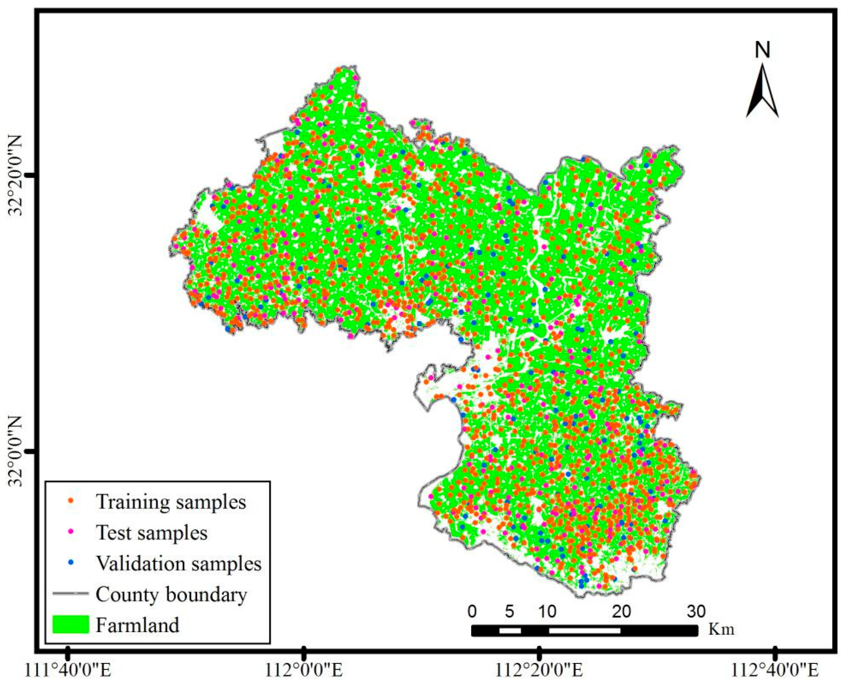
Training set generation

Based on Table 1 and the results of the national farmland quality grades, the original sample set was generated from randomly selected farmland patches of different quality grades in Xiangzhou, and adjusted according to the spatial location of the samples to achieve uniform distribution, with a total of 1590 samples selected. Then, 70% of the data was randomly selected as a training sample (1110), 20% as a test sample (320), and 10% as a validation sample (160), as shown in Figure 5. First, 1590 training sets equal to the number of samples were chosen randomly with playback from the training sample. Second, the indicator attribute values were sampled and learned multiple times until the average error rate was stabilized using R to access the random forest library. Then, based on the mapping of quality index to attribute values for each indicator, a decision tree was constructed to output the rules for predicting the quality index of farmland. The above steps were repeated to construct different decision trees for training the RF model for farmland quality assessment, which were applied to the assessment of Xiangzhou in 2018. The results showed that the coefficient of determination (R²) for the training sample was in the range of 0.7727–0.9483 (

Table 4. Corresponding errors for different values of n and their R².

Number (n)	Error	R2
1	0.000211	0.7727
2	0.0000830	0.91
3	0.0000620	0.9332
4	0.0000548	0.9409
5	0.0000528	0.9432
6	0.0000499	0.9462
7	0.0000480	0.9483
8	0.0000495	0.9466
9	0.0000494	0.9468
10	0.0000502	0.9459
11	0.0000493	0.9469
12	0.0000482	0.948
13	0.0000497	0.9464
14	0.0000507	0.9454

) and was significant at the 5% level, with high prediction accuracy.

(2)

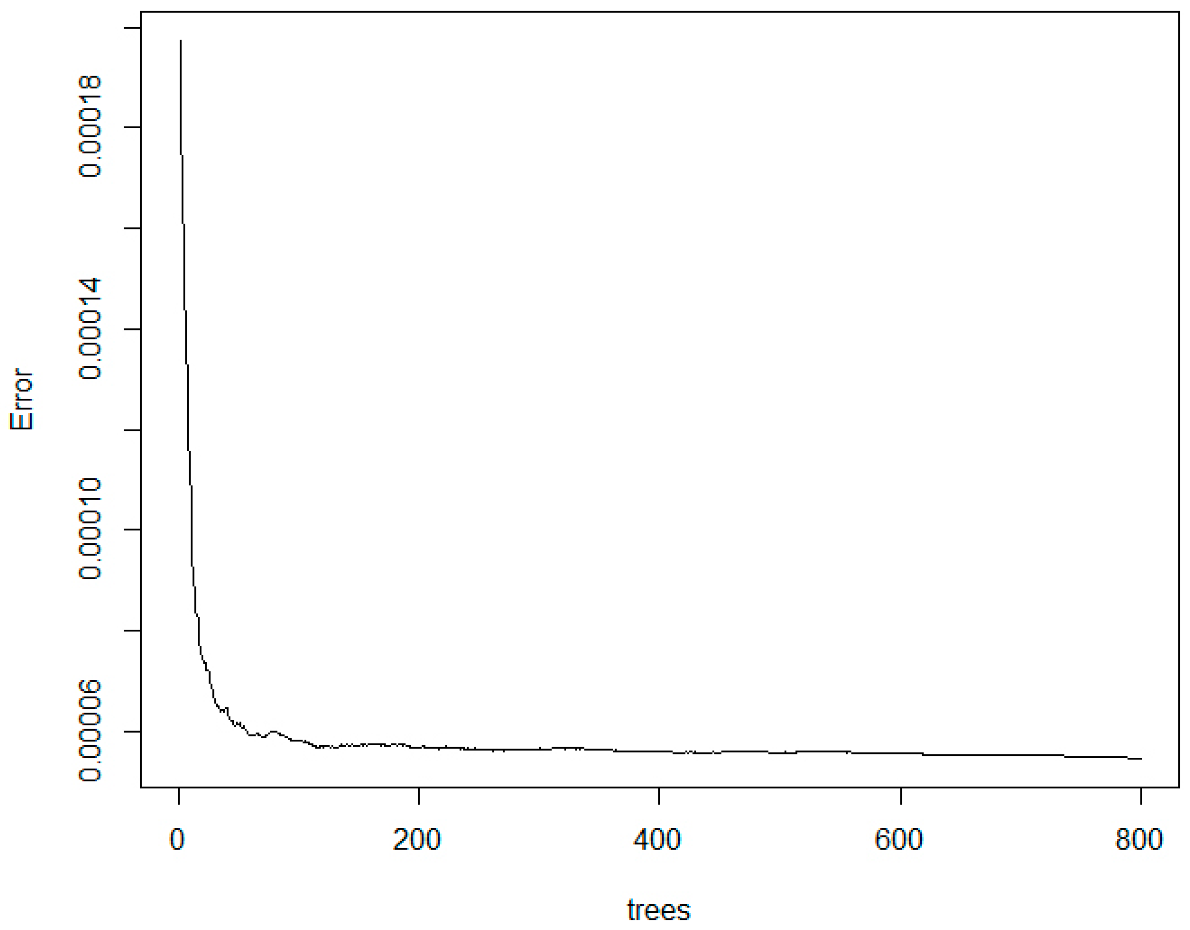
Parameter optimization

The random forest package in R was used to apply out-of-bag (OOB) data for unbiased estimation of the accuracy of the RF model in this study. After debugging and parameter sensitivity analysis, the OOB error tended to stabilize when the number of decision trees was greater than 200 (Figure 6). The overall error of the model and the coefficient of determination (R²) were compared by adjusting the number of assessment indicators (Table 4) to determine the optimal segmentation node (n). The error was minimized and R² was maximized when the number of node segments (n) was 7.

For BPNN, the neural-net package in R was used to train neural networks using backpropagation. In the main parameter settings, the hidden layer was 5, the number of random seeds was 2000, the initial weight range was 0–1, the weight adjustment rate was 0.1, the minimum target error was 0.01, the learning rate was 0.05, the maximum number of iterations was 1000, the number of training repetitions was 1, the impulse coefficient was 1.2, the error type was sse, the activation function was tanh, and the output form was linear.

(3)

Determination of weighted indicators

To avoid overfitting assessment indicators, the importance of evaluating indicators was determined in the construction of the RF model by calculating the reduced value of the Gini index at node splitting based on out-of-bag (OOB) data not involved in constructing the decision trees, which is implemented as follows.

The Gini index expresses the impurity of a node, which is defined as the following in Equation (3):

$$Gini(n)=1-{{\displaystyle \sum _{i=1}^j\left[p(i|n)\right]}}^2$$

(3)

where $p(i|n)$ is the probability of farmland quality. When Gini(n) is 0, it means that the training data at n nodes are of the same quality grade of farmland. A larger Gini(n) means that the training data at n nodes are more scattered, and the nodes need to be further divided.

The original split Gini index of the kth decision tree is assumed to be Gini g_k. The new Gini index (Gini g_kⁱ) is recalculated by performing random series changes on the ith assessment indicator (Z) of the OOB data. Then the weight of indicator Z in the corresponding single decision tree (WG_i) is denoted as Gini g_k − Gini g_kⁱ. The weight of the ith assessment indicator (RFW_i) is the average of all decision trees in the RF, which is calculated as follows in Equations (4) and (5):

$$W{G}_i=\left|\raisebox{1ex}{${\displaystyle \sum _{i=1}^m(Gin{i}_{gk}-Gin{i}_{g_k^i})}$}\!\left/ \!\raisebox{-1ex}{$N$}\right.\right|$$

(4)

$$RF{W}_i=\raisebox{1ex}{$W{G}_i$}\!\left/ \!\raisebox{-1ex}{${\displaystyle \sum _{i=1}^{m}W{G}_i}$}\right.$$

(5)

In the formulas, WG_i is the reduced value of the Gini index, m is the number of assessment indicators, and RFW_i is the weight of the ith assessment indicator.

(4)

Calculation of farmland quality index

The best RF model between each assessment indicator of the independent variable and the farmland quality of the dependent variable according to the linear decomposition rules of the decision tree mapping was constructed, and the weight of each assessment indicator was calculated. The test set was then entered into each RF decision tree. The sum of the index values at each leaf node multiplied by their weights is the farmland quality index for that tree. Finally, the farmland quality index was obtained by calculating the average value of the index for each decision tree.

Comparison Methods

Current methods of assessing farmland quality can be broadly divided into two categories: conventional weighting and machine learning. Therefore, to more accurately verify the reliability and superiority of the machine learning (RF model) in this study, we compared the performance of EW (represented as the conventional weighting method) and BPNN (represented as the machine learning method).

(1)

Compared to other conventional weight assessment methods, EW is an objective weight method that is free from human influence and has the most basic and simple model construction, which enables better interpretation of assessment results. Therefore, EW was chosen as a typical representative of conventional weight-assessment methods. The fundamental principle of EW is to calculate objective weight based on the amount of variability in the indicator. The less information entropy there is, the greater the variation and weight of the indicator. Due to the wide application of this method, it was not repeated in this paper concerning the specific calculation procedure [19].

(2)

BPNN and SVM are classical representatives of machine-learning methods, both of which are more stable and flexible than conventional weight-assessment methods. However, compared to BPNN, the choice of SVM parameters poses greater constraints to construction, which largely limits the depth of research and breadth of SVM application. Artificial neural networks tend to mature in farmland quality assessment studies, mainly using BPNN or its deformed form model. Therefore, in this study, BPNN was chosen as a typical representative of machine-learning methods, and we attempted to construct a five-layer BPNN structure for farmland quality assessment model using R.

3. Results

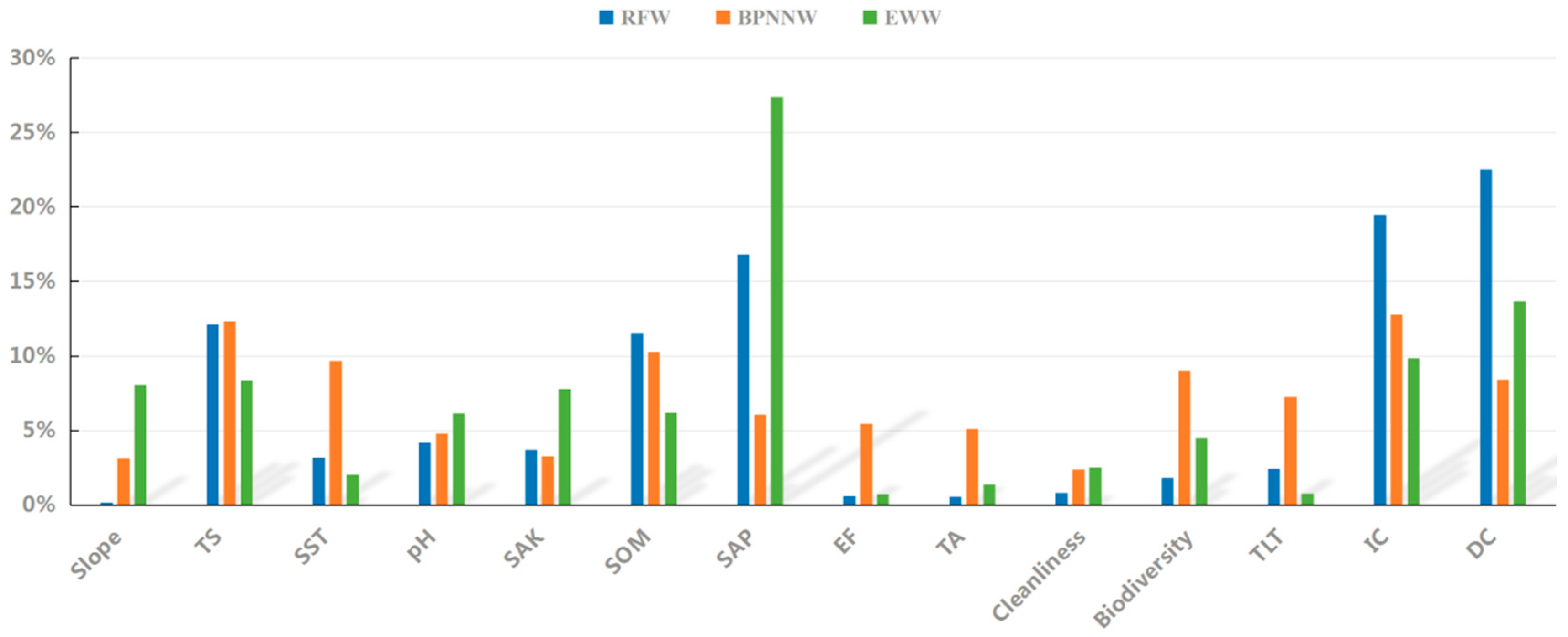
3.1. Analysis of Indicator Weights Determined Based on Three Models

The RF weight (RFW) for each assessment indicator was calculated based on the reduction in the Gini index produced by RF during the training process. The drainage capacity, irrigation capacity, soil available phosphorus, topographic site, and soil organic matter were identified as the five most important indicators affecting farmland quality in RFW, with a total weight of 82.41% (Figure 7). Slope, traffic accessibility, and ease of farming were the three indicators that had the least impact on farmland quality, with a weight of only 1.35%. Meanwhile, the weight of each indicator in BPNN (BPNNW) and EW (EWW) were calculated. The BPNNW identification was more balanced, with drainage capacity and irrigation capacity being more important, and slope and cleanliness the least important indicators. EWW identified soil available phosphorus as the most important indicator, and ease of farming as the least important. Thus, the difference between RFW and BPNNW was small in terms of indicator weight values, while the difference between EWW and BPNNW was significant. Adequate drainage and irrigation capacity are important for farmland productivity, soil available phosphorus and soil organic matter reflect the fertility of farmland, and topography is an important factor limiting farmland productivity in hilly areas. Therefore, they all have an important impact on farmland quality. Regularity among slope, traffic accessibility, ease of farming, and the remaining indicators is not sufficiently evident. Thus, they were identified by RF as the least-important impact factors.

From the basic principle of the method, EWW calculates the indicator weight based on the objective trend of the indicator attribute values, while RFW and BPNNW reflect the intrinsic connection between the quality of farmland and each indicator and calculate the indicator weight based on the reduced value of the Gini coefficient, which is more in line with the complexity and nonlinearity of the farmland quality system. Therefore, RFW and BPNNW should have more explanatory power for the indicators. Meanwhile, from the results of the run program, the RF average error was 0.0019, the average prediction accuracy was 93.01%, and the convergence time was 4.43 s; while the BPNN average error was 0.0057, the average prediction accuracy was 88.19%, and the convergence time was 5.87 s. It can be seen that compared to BPNN, RFW was more interpretable, more accurate in predicting indicators, and faster at processing data, and its weights were more accurate in fitting the interrelationships between indicators and assessment objects.

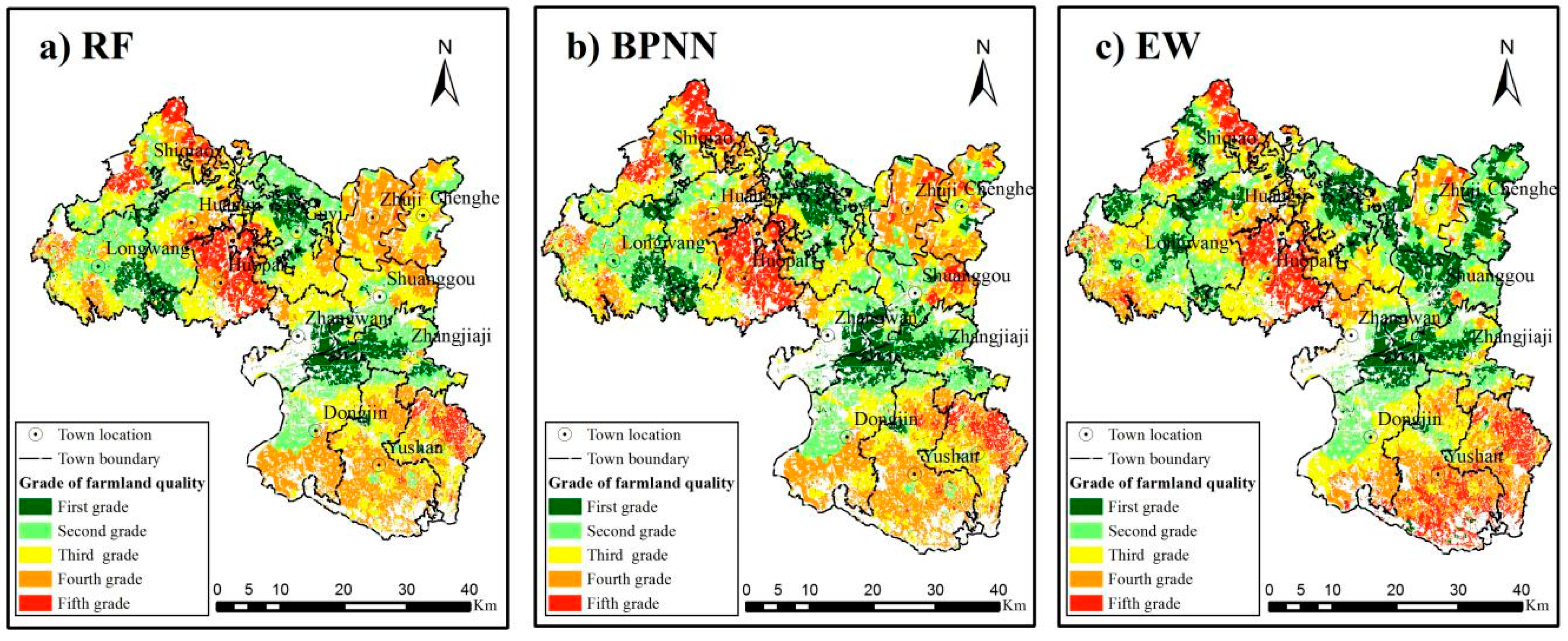
3.2. Analysis and Comparison of Results of Farmland Quality Assessment

According to RFW, BPW, and EWW, the cultivated quality index was calculated for Xiangzhou in 2018. Using the natural fracture method of ArcGIS, farmland quality was classified into five grades, in descending order from first to fifth. The results of the farmland quality assessment based on RF, BPNN, and EW are shown in Figure 8 and

Table 5. Acreage and proportion of grades for the three methods of evaluating grades of farmland quality.

Model	Area/Proportion	First Grade	Second Grade	Third Grade	Fourth Grade	Fifth Grade
Random forest (RF)	Area/hm2	14,680.44	41,365.19	48,912.49	46,704.13	13,594.74
	Proportion/%	8.88	25.03	29.60	28.26	8.23
Backpropagation neural network (BPNN)	Area/hm2	19,163.23	40,484.52	43,261.89	45,500.65	16,846.71
	Proportion/%	11.60	24.50	26.18	27.53	10.19
Entropy weight (EW)	Area/hm2	27,558.40	42,137.51	43,976.13	32,252.10	19,332.85
	Proportion/%	16.68	25.50	26.61	19.52	11.70

.

3.2.1. Analysis of RF Assessment Results

From an overall perspective, the average farmland quality index in Xiangzhou was 0.8275, which indicates higher quality. The proportion of second- and third-grade farmland was larger, accounting for 54.63%, and the proportions of first- and fifth-grade farmland were smaller, at 8.88% and 8.23%, respectively, which shows that the farmland quality grade was in a normal distribution (Figure 8a). In terms of the average farmland quality index, Zhangjiaji, Zhangwan, Shuanggou, Guyi, and Longwang had the highest values, at 0.8517, 0.8475, 0.8395, 0.8375, and 0.8356, respectively; while the average values in Yushan, Huopai, and Huanglong were relatively low, at 0.8175, 0.8149, and 0.8094, respectively. As far as different land types were concerned, the average index of farmland quality was 0.8286, 0.8282, and 0.8267 for paddy fields, irrigated land, and dry land, respectively, which shows that paddy fields had the best quality. In addition, the spatial distribution of farmland quality in Xiangzhou was uneven, and was greatly influenced by topography and socioeconomic development, showing an overall distribution pattern of high in the north-central part and low in the south (Figure 8a). Higher-quality farmland was mainly distributed in Zhangjiaji, Zhangwan, and Shuanggou in the central part and Longwang and Guyi in the north, while lower-quality farmland was mainly distributed in Yushan and Huanglong in the south. The central part of Xiangzhou belongs to the alluvial plain of the Han River, with flat terrain and fertile soil, mainly loam and sand. There are certain sources of contamination in the region due to economic development, which affects farmland productivity. However, there are more rivers, better field drainage and irrigation facilities, and richer biodiversity in this area. Therefore, in general, the fertile alluvial plain is suitable for the development of cultivated agriculture. The northern and southern parts of Xiangzhou have hillock landforms and low hilly areas with high terrain and steep slopes that are prone to soil erosion and have relatively poor soil. Although the farmland area is large, the level of land use is low due to fewer water sources and poor drainage and irrigation facilities resulting from extensive farming, which make this farmland suitable for subtropical cash crops.

3.2.2. Comparison of Assessment Results

Overall, as far as the average farmland quality index for Xiangzhou was concerned, RF > BPNN > EW, with values of 0.8275, 0.8271, and 0.7532, respectively. Thus, the farmland quality in Xiangzhou was higher. For the average farmland quality index of each town, the assessment results of RF and BPNN were relatively similar, but there were also significant relative differences in terms of local regions. As can be seen in Table 5, the percentage of area of each measured farmland quality grade based on RF was closer to that of BPNN, but differed significantly from that of EW; the most significant difference was for first grade, which was 8.88% for RF and 16.68% for EW. In Figure 8a, it can be seen that first-grade farmland based on RF was mainly distributed in Zhangwan, Guyi, and Longwang, while that based on EW was mainly distributed in Shuanggou, Chenghe, Guyi, Longwang, and Shiqiao (Figure 8c). Shuanggou and Chenghe are industrial towns in Xiangzhou with high urbanization and high intensity of farmland use, and existing studies have shown that the heavy-metal element content of farmland soil around the towns is high overall, so it is unreasonable for the farmland to be identified as first-grade land [44,55]. The topography of Shiqiao is high and the soil water and fertilizer retention ability is poor, so theoretically, the quality grade of farmland should be lower, which is consistent with the existing research results [56]. RF identified Shuanggou as having high-grade farmland quality (Figure 8a), while BPNN identified it as low grade (Figure 8b). Shuanggou has a flat terrain, fertile soil, numerous rivers, abundant water sources, and relatively complete irrigation and drainage facilities, and its natural geographical conditions are advantageous for the development of arable agriculture. Therefore, this town should, theoretically, be an area of high-quality farmland. This analysis is also empirically supported by numerous studies [57]. The results of the EW assessment differed greatly from the other two methods. Areas with higher quality farmland were mainly distributed in Zhangwan, Shuanggou, Chenghe, and Prison Farm, while areas with lower-quality farmland were mainly distributed in Huopai, Yushan, and Huanglong (Figure 8c).

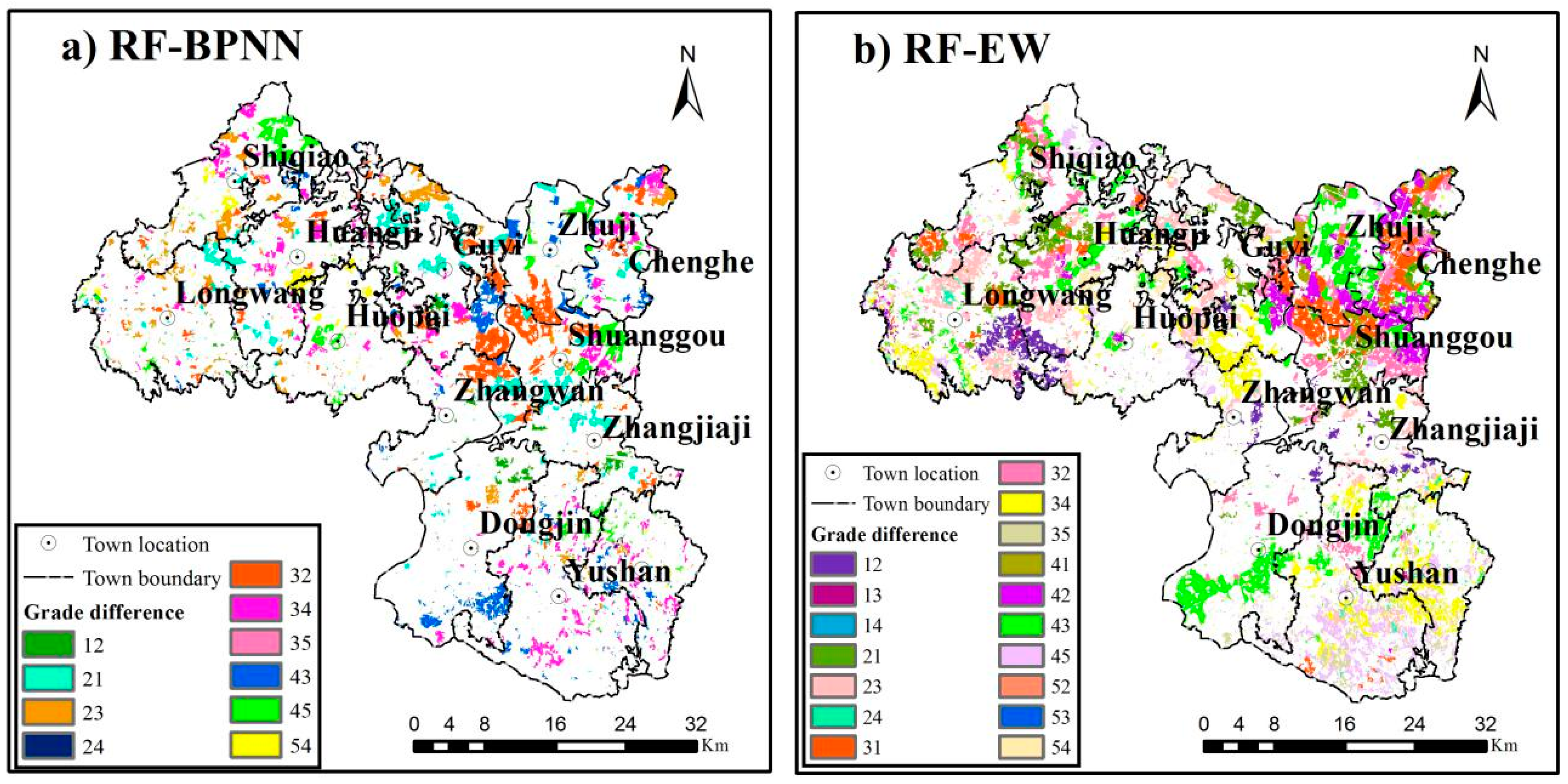
3.3. RF Model Reasonableness Test

To further measure the rationality of the RF model for evaluating farmland quality, the consistency of the results of RF, BPNN, and EW was compared and analyzed in this study. The superiority of RF was revealed by four indices: mean absolute error (MAE), standard mean square error (MSE), coefficient of determination (R²), and significance.

3.3.1. Consistency Test

The validity of the RF model was verified by analyzing the differences among the assessment results of RF, BPNN, and EW in the following process. First, the five grades of farmland quality were assigned values of 1 to 5, respectively. Second, using the raster calculator tool of ArcGIS, the assigned values of farmland quality grade evaluated by RF were multiplied by 10 and summed with those evaluated by BPNN and EW to obtain a two-digit result. If the two digits were the same, then RF was the same as BPNN and EW; otherwise, it was different. The spatial distribution of the differences between the results of farmland quality assessment for RF and BPNN and between RF and EW are shown in Figure 9, where the first number of the difference marker is the RF grade and the second number the BPNN or EW grade. For example, a value of 13 means that RF identified the area as first-grade farmland and BPNN or EW identified it as third grade, while 31 means that RF identified the area as third-grade farmland and BPNN or EW identified it as first grade.

In the comparison of results between RF and BPNN, the number of errors as a percentage of the total sample was 22.74%, mainly concentrated in one grade of difference—12, 21, 23, 32, 34, 43, 45, 54—whose ratio was as high as 99.36% (Figure 9). From the results of the comparison between RF and EW, the proportion of error points among the total number of samples was significantly higher, reaching 48.24%, and the difference between the two assessments was mainly concentrated in one grade—12, 21, 23, 32, 34, 43, 45, 54—whose error points account for about 79.67%. Thus, the assessment results of RF and BPNN were in high agreement. In these errors, EW identified areas of higher quality that RF and BPNN identified as lower. Some of these areas were relatively high terrain, with poor soil fertility and mediocre drainage and irrigation facilities, where the farmland quality was largely constrained by topography and soil fertility and was, theoretically, relatively low. EW identified areas of lower farmland quality that RF and BPNN identified as higher. Some of these areas were flat, with relatively fertile soil and rich biodiversity and theoretically high-quality farmland. Obviously, the assessment results of RF and BPNN were more convincing compared to EW, so their superiority was further compared.

3.3.2. Superiority Test

To validate the superiority of RF, the test datasets were selected to construct the RF and BPNN models for assessing farmland quality and to compare to the results of the assessment above. As shown in

Table 6. Error analysis of assessment results.

Model	MAE	MSE	R2	Significance
RF	0.009	0.012	0.8145	0.000
BPNN	0.021	0.026	0.4594	0.213

, in RF, the MAE was 0.009 and the MSE was 0.012, both less than in BPNN. The coefficient of determination (R²) of RF was 0.8145, greater than BPNN. The F-test showed that RF passed the 5% level of significance, while BPNN was not significant. Thus, compared to other assessment methods, RF has the lowest generalization error, highest accuracy, better stability, and better assessment capability. RF may be preferred over BPNN for farmland quality assessment.

4. Discussion

4.1. Construction of a Comprehensive Assessment Index System for Farmland Quality

The construction of the index system is the focus of quality-assessment research [24]. How to reasonably determine an assessment index system based on different purposes is the primary problem of farmland quality assessment. Kong et al. [17] established a pressure–state–effect–response assessment system based on changes in farmers’ land-use objectives. Chen et al. [58] constructed an element–demand–regulation assessment system for slope farmland based on the minimum dataset. Due to the complexity of farmland quality systems, the topography, physical and chemical properties of the soil, land use, economic level, and ecological environment should be fully considered in the selection of indicators. However, soil factors and topography as indicators were selected only in the traditional farmland quality assessment [47]. The ecological conditions of farmland have not been adequately considered in current research [59]. Therefore, it is particularly important to establish an index system that considers both socioeconomic factors and the ecological environment. In this study, a comprehensive assessment index system was built to characterize the diversity of farmland ecosystems in terms of their natural, socioeconomic, and ecological environment conditions.

Slope, topographic site, surface soil texture, soil organic matter, tillage-layer thickness, soil pH, soil available phosphorus, and soil available potassium were chosen to represent natural conditions based on the natural properties of farmland in this study. Soil is an important natural resource with a diversity of ecological functions, and is the basis for agricultural development [60]. Slope, topographic site, and surface soil texture are chosen to assess the suitability of farmland [61]. Tillage-layer thickness is used as an important indicator of land degradation [62]. Soil organic matter, pH, available phosphorus, and available potassium have been used to evaluate soil fertility quality [63]. Soil organic matter is the main source of crop nutrition, and is an important indicator of soil fertility [64,65]. Soil pH is one of the most important factors affecting the effectiveness of soil nutrients, which is closely related to fertilizer absorption efficiency, and most crops grow best when soil pH is 6.5–7.5 [66]. Soil available phosphorus and potassium play important roles in plant growth, and are the main fertilizers applied to plants in agricultural production [67,68].

In the 1980s, the Land Evaluation and Site Assessment (LESA) system established by the Soil Conservation Service (SCS) in Washington of USA emphasized the important role played by socioeconomic conditions in farmland quality assessment [69]. In this study, drainage capacity, irrigation capacity, ease of farming, and traffic accessibility were chosen as socioeconomic indicators. Water resource is an important factor influencing crop yields [70,71]. A proper drainage and irrigation pattern not only improves drainage capacity, but also maintains the soil moisture of the farmland [72]. Accessibility is regarded as having an influence on the spatial pattern of land use [73], which is calculated by the distance from patches to roads [74,75], and it was reflected in the ease of farming and road accessibility in this study.

Over the past decade, China’s agricultural development has shifted from the pursuit of increased yields to a concern for the ecological safety of farmland [76]. Therefore, ecological factors need to be considered in the assessment of farmland quality [77,78]. In this study, biodiversity and cleanliness indicators were selected to measure ecological quality based on previous studies [79]. Biodiversity is an important indicator of farmland ecological values, and is usually composed of genetic, species, and ecosystem diversity [80]. In terms of the data acquisition of biodiversity indicators, due to the limitation of experimental conditions in the study area, it was not possible to analyze them quantitatively, and their levels were only analyzed qualitatively using the percentage of earthworms in the soil, and further in-depth study is needed. Cleanliness reflects the environmental condition of the soil, and it has been used as an important indicator of soil ecological safety [81]. In the acquisition of cleanliness index data, due to the lack of data, we failed to start from the essence of environmental quality and select pollution elements for analysis, and only used a few substitute indicators that were not comprehensive enough for a description of ecological environmental quality, and require further exploration and in-depth study.

4.2. The Influence of Research Scale on Indicator Selection

Due to the large differences in the selection of assessment indicators and access to basic data, the focus and accuracy of the results of farmland quality assessment at different scales also differ greatly; i.e., the assessment has spatial scale effects [82]. Kong et al. [83] argued that farmland quality has significant scale variability, with some characteristics acting at the micro level and some at the macro level. The smaller the assessment scale, the more assessment indicators are available and the higher the accuracy of indicators, and thus the finer the degree of assessment, though the applicability of results is often narrower. As the assessment scale is enlarged, relatively fewer indicators are available, and their accuracy is reduced, and the results reflect the macroscopic characteristics of farmland quality, but the applicability of large-scale farmland quality assessment results is also wider [84]. From the selection of assessment indicators at different scales, the small-scale farmland quality assessment index system is based on soil attribute indicators, and its process focuses on assessing the natural quality of farmland, while at large scale, macro factors are selected from natural conditions, land use level, and economic level to build an assessment system [85]. The physicochemical, biological, and health characteristics of soil, as well as topographical conditions, are the main factors that influence the productive potential of farmland. Realistic farmland quality is obtained by analyzing the impact of land use and economic levels on the productive potential. The combination of field surveys and remote sensing is an important tool for evaluating land quality.

The county is the basic administrative unit for farmland management in China, and farmland resource management and conservation policies can be formulated based on the results of quality assessment [86]. In this study, the farmland quality assessment system was built from four dimensions of terrain, soil conditions, socioeconomics, and ecological environment in Xiangzhou. The micro-indicators of social production and ecology were selected. In reflecting the public’s demand for diversified farmland function, this research can provide a theoretical reference for national farmland assessment. It could also provide technical support for farmland management in Xiangzhou. More importantly, the method could be applied to similar national and regional cultivated quality assessments. However, as influenced by the scale effect of the assessment, there are problems such as the lack of comparability of different scales of farmland quality assessment index systems and results [83,84]. Research on the construction of a multiscale farmland quality assessment index system and the establishment of an assessment model and scale conversion need to be further developed.

4.3. Construction of Farmland Quality Assessment Model

How to reasonably identify the weight of indicators is central to the construction of a farmland quality assessment model [20]. Lin et al. [42] used the random forest algorithm, with the average standard yield as the dependent variable and the influence factor as the independent variable, to construct a regression model to determine indicator weights and compare the accuracy of this determination with that of Delphi. To further verify the reliability and superiority of the RF model, typical samples of the study area were selected, and three deep machine-learning models were selected for training, namely entropy weight (EW), backpropagation neural network (BPNN), and random forest (RF), and the results of farmland quality assessment were output through simulation. Comparing training accuracy in terms of the BPNN and EW measurements of the weights of assessment indicators may not be in line with the actual situation: RF can more effectively decompose indicators that have a nonlinear relationship with the assessment object into leaves with linear relationships and determine the weights of the indicators in the operation process, which is associated with higher indicator interpretation ability, and the assessment results are more ideal and in line with objective reality. In addition, the selection of training samples is crucial; different samples have an impact on the final evaluation results, and this study only used the uniform method to select samples, so the next step can select samples in different ways, and an in-depth comparative analysis can be conducted.

Due to the complexity of the factors influencing the quality of farmland, whether the assessment model is properly constructed during actual production will directly affect the accuracy of the comprehensive assessment of farmland quality. Furthermore, the indicator weights are automatically generated during the training process based on the rules of decomposition of the attribute values of real data, whereas the assessment indicators change with socioeconomic development. Therefore, the model constructed in this study is not applicable to the future assessment of farmland quality. Further improvement of the RF model to improve the accuracy of farmland quality assessment will be the focus and challenge of subsequent research, and will take into account the actual conditions of the study area and the natural and socioeconomic factors that affect farmland quality.

5. Conclusions

In this study, an RF model for farmland quality assessment was constructed and applied to the assessment of Xiangzhou in Hubei Province in 2018, based on the construction of decision trees using bootstrap. BPNN and EW were used as a comparison to verify the advantages and disadvantages of the three models. The main findings were as follows:

(1)

The results showed that as far as the average farmland quality index in Xiangzhou is concerned, RF > BPNN > EW, and the assessment results of RF and BPNN showed more similar spatial distribution, while that of EW differed greatly. From a practical point of view, the assessment result of RF was more in line with the local natural conditions and socioeconomic development and was more objective. In terms of assessment accuracy, the RF model had the advantage of digging deeper into the nonlinear relationship between the indicators and the evaluated object. Its generalization ability was stronger, its assessment accuracy was higher, and its assessment results were more in line with the spatial distribution of farmland quality, which were consistent, typical, and superior to those of BPNN and EW.

(2)

The quality of farmland in Xiangzhou was generally high, with a large area being of second- and third-grade quality, accounting for 54.63% of the total farmland area, and the grades basically conformed to a positive distribution trend. From the distribution point of view, the spatial distribution of farmland quality in Xiangzhou was unbalanced, influenced by the topography and socioeconomic development level and showing an obvious geographical distribution pattern, with overall characteristics of high in the north-central area and low in the southern area. The distribution of farmland quality grades also differed greatly among regions.

(3)

To a certain degree, due to the complexity, uncertainty, and nonlinearity of farmland quality systems, farmland quality from the perspective of the RF model was researched as an expansion of assessment methods, based on the theories and methods of artificial intelligence technology, which can improve the accuracy and quantitative level of farmland quality assessment. This study provides a new assessment method for farmland quality that can support the formulation of rational and effective management policies toward realizing the sustainable use of farmland resources. Moreover, the assessment model constructed in this study could be used as a reference for similar countries and regions.

References

1. Jiang, G.; Zhang, R.; Ma, W.; Zhou, D.; He, X. Cultivated land productivity potential improvement in land consolidation schemes in Shenyang, China: Assessment and policy implications. Land Use Policy 2017, 68, 80–88. [Google Scholar] [CrossRef]
2. Kong, X. China must protect high-quality arable land. Nature 2014, 506, 7. [Google Scholar] [CrossRef] [PubMed]
3. Wang, N.; Zu, J.; Li, M.; Zhang, J.Y.; Hao, J.M. Spatial Zoning of cultivated land in Shandong Province Based on the Trinity of Quantity, Quality and Ecology. Sustainability 2020, 12, 1849. [Google Scholar] [CrossRef] [Green Version]
4. Xiao, Q.; Zong, Y.T.; Lu, S.G. Assessment of heavy metal pollution and human health risk in urban soils of steel industrial city (Anshan), Liaoning, Northeast China. Ecotoxicol. Environ. Saf. 2015, 120, 377–385. [Google Scholar]
5. Burges, A.; Epelde, L.; Garbisu, C. Impact of repeated single-metal and multi-metal pollution events on soil quality. Chemosphere 2015, 120, 8–15. [Google Scholar] [CrossRef]
6. Jin, X.B.; Shao, Y.; Zhang, Z.H.; Resler Lynn, M.; Campbell, B.J.; Chen, G.; Zhou, Y.K. The evaluation of land consolidation policy in improving agricultural productivity in China. Sci. Rep. 2017, 7, 2792. [Google Scholar] [CrossRef] [Green Version]
7. Zheng, H.; Huang, H.; Zhang, C.; Li, J. National-scale paddy-upland rotation in Northern China promotes sustainable development of cultivated land. Agric. Water Manag. 2016, 170, 20–25. [Google Scholar] [CrossRef]
8. Cao, Y.; Bai, Z.; Zhou, W.; Wang, J. Forces driving changes in cultivated land and management countermeasures in the Three Gorges Reservoir Area, China. J. Mt. Sci. 2013, 10, 149–162. [Google Scholar] [CrossRef]
9. Zhao, X.; Ye, Y.; Zhou, J.; Liu, L.; Hu, Y. Comprehensive assessment of cultivated land quality and sensitivity analysis of index weight in hilly region of Pearl River Delta. Trans. Chin. Soc. Agric. Eng. 2017, 33, 226–235. [Google Scholar]
10. Yang, J.; Wang, L.; Song, F.; Fan, P. Major Grain-Producing Areas Of Cultivated Land Quality Influence Factors And Grain Production Capacity Relationship Analysis. Chin. J. Agric. Res. Reg. Plan. 2017, 38, 15–22. [Google Scholar]
11. Yuan, X.; Shao, Y.; Wei, X.; Hou, R.; Ying, Y.; Zhao, Y.; Li, R. Study on the potential of cultivated land quality improvement based on a geological detector. Geol. J. 2018, 53, 387–397. [Google Scholar] [CrossRef]
12. Song, W.; Pijanowski, B. The effects of China’s cultivated land balance program on potential land productivity at a national scale. Appl. Geogr. 2014, 46, 158–170. [Google Scholar] [CrossRef]
13. Li, X.; Zhang, W.; Peng, Y. Grain Output and Cultivated Land Preservation: Assessment of the Rewarded Land Conversion Quotas Trading Policy in China’s Zhejiang Province. Sustainability 2016, 8, 821. [Google Scholar] [CrossRef]
14. Bui, E.N.; Henderson, B.L.; Viergever, K. Knowledge discovery from models of soil properties developed through data mining. Ecol. Model. 2006, 191, 431–446. [Google Scholar] [CrossRef]
15. Parisi, V.; Menta, C.; Gardi, C.; Jacomini, C.; Mozzanica, E. Microarthropod communities as a tool to assess soil quality and biodiversity: A new approach in italy. Agric. Ecosyst. Environ. 2005, 105, 323–333. [Google Scholar] [CrossRef]
16. Calabrese, J.; Ladisa, G.; Ladisa, G.; Otekhile, A. Impacts of land cover change on soil quality of manmade soils cultivated with table grapes in the Apulia Region of south-eastern Italy. Catena 2014, 121, 13–21. [Google Scholar]
17. Kong, X.B.; Liu, L.W.; Qin, J. Arable Land Evaluation Based on the Household Land Use Behavior in Daxing District of Beijing. Acta Geogr. Sin. 2008, 63, 856–868. [Google Scholar]
18. Zhu, C.M.; Hao, J.M.; Chen, L.; Deng, S.Y.; Liu, P.H. Well-facilitied capital farmland construction based on cultivated land comprehensive quality. Trans. Chin. Soc. Agric. Eng. 2015, 3, 233–242. [Google Scholar]
19. Gu, Z.; Wang, Y.; Sun, Y.; Ding, J. Application of entropy-weight TOPSIS model in synthetical quality assessment of Angelica sinensis growing in Gansu Province. J. Chin. Med. Mater. 2014, 37, 1549–1553. [Google Scholar]
20. Nie, Y.; Zhou, Y.; Qian, J.; Huang, J. Evaluation of Cropland Quality in Jingzhou’s Urban Fringe. Res. Sci. 2008, 6, 121–126. [Google Scholar]
21. Garcia-Melon, M.; Ferris-Onate, J.; Aznar-Bellver, J.; Aragones-Beltran, P.; Poveda-Bautista, R. Farmland appraisal based on the analytic network process. J. Glob. Optim. 2008, 42, 143–155. [Google Scholar] [CrossRef]
22. Meng, X.; Shi, F. An extended data envelopment analysis for the decision-making. J. Inequal. Appl. 2017, 1, 240. [Google Scholar] [CrossRef] [PubMed] [Green Version]
23. Ye, Y.; Zhao, X.; Hu, Y. Evaluation of cultivated land Quality in Pearl River Delta Based on GA-BP Neural Network. Ecol. Environ. Sci. 2018, 27, 964–973. [Google Scholar]
24. Zhu, M.; Liu, S.; Xia, Z.; Wang, G.; Hu, Y.; Liu, Z. Crop Growth Stage GPP-Driven Spectral Model for Evaluation of Cultivated Land Quality Using GA-BPNN. Agriculture 2020, 10, 318–333. [Google Scholar] [CrossRef]
25. Li, L. Model of Productivity of Cultivated Land Based on Improved-SVM. J. Shenyang Agric. Univ. 2012, 43, 126–128. [Google Scholar]
26. Qie, R.Q.; Guan, X.; Yan, X.J.; Dou, S.X.; Zhao, L. Method and its application of natural quality evaluation of arable land based on self-organizing feature map neural network. Trans. Chin. Soc. Agric. Eng. 2014, 30, 298–305. [Google Scholar]
27. Gao, Y. Research on Natural Quality Evaluation of Arable Land Based on BP Neural Network. Master’s Thesis, Central China Normal University, Wuhan, China, 2012. [Google Scholar]
28. Shekofteh, H.; Masoudi, A. Determining the features influencing the-S soil quality index in a semiarid region of Iran using a hybrid GA-ANN algorithm. Geoderma 2019, 355, 113908. [Google Scholar] [CrossRef]
29. Gayen, A.; Pourghasemi, H.R.; Saha, S.; Keesstra, S.; Bai, S.B. Gully erosion susceptibility assessment and management of hazard-prone areas in India using different machine learning algorithms. Sci. Total Environ. 2019, 668, 124–138. [Google Scholar] [CrossRef]
30. Lai, H.S.; Wu, C.F. Productivity Evaluation of Standard Cultivated Land Based on Rough Set and Support Vector Machine. J. Nat. Res. 2011, 26, 2141–2154. [Google Scholar]
31. Wang, H.; Luo, P.; Zhao, Z.; Nie, K. Establishment of agricultural land appraisal model based on deep belief network. Trans. Chin. Soc. Agric. Eng. 2018, 34, 263–271. [Google Scholar]
32. Hassoun, M. Fundamentals of Artificial Neural Networks. Proc. IEEE 2002, 84, 906. [Google Scholar] [CrossRef]
33. Herzog, S.; Tetzlaff, C.; Wrgtter, F. Evolving artificial neural networks with feedback. Neural Netw. 2020, 123, 153–162. [Google Scholar] [CrossRef] [PubMed]
34. Chen, G.; Du, J.B.; Sun, L.; Zhang, W.; Xu, K.; Chen, X.T.; Reed, G.; He, Z. Nonlinear Distortion Mitigation by Machine Learning of SVM Classification for PAM-4 and PAM-8 Modulated Optical Interconnection. J. Lightwave Technol. 2018, 36, 650–657. [Google Scholar] [CrossRef]
35. Liaw, A.; Wiener, M.; Liaw, A. Classification and Regression with Random Forest. R News 2002, 23, 18–22. [Google Scholar]
36. Chunrong, M.; Falk, H.; Guo, Y.; Han, X.; Wen, L. Why choose Random Forest to predict rare species distribution with few samples in large undersampled areas? Three Asian crane species models provide supporting evidence. PeerJ 2017, 5. [Google Scholar] [CrossRef] [Green Version]
37. Lindner, C.; Bromiley, P.; Ionita, M.; Cootes, T. Robust and accurate shape model matching using Random Forest Regression-Voting. IEEE Trans. Pattern Anal. Mach. Intell. 2015, 37, 1862–1874. [Google Scholar] [CrossRef]
38. Chen, D.L.; Lu, X.H.; Kuang, B. Measurement of cultivated land utilization efficiency: Construction and application of random forest. J. Nat. Res. 2019, 34, 1331–1344. [Google Scholar]
39. Khamoshi, E.; Sarmadian, F.; Keshavarzi, A. Digital Soil Mapping Using Random Forest Model and Land Suitability Evaluation for Abyek Region, Qazvin Province, Iran. J. Range Watershed Manag. 2019, 71, 885–899. [Google Scholar]
40. Bhowmik, A.; Kukal, S.S.; Saha, D.; Sharma, H.; Kalia, A.; Sharma, S. Potential Indicators of Soil Health Degradation in Different Land Use-Based Ecosystems in the Shiwaliks of Northwestern India. Sustainability 2019, 11, 3908. [Google Scholar] [CrossRef] [Green Version]
41. Chen, X.F.; Ren, X.N.; Zhang, C.; Xian, C.L.; Feng, X.K.; Ma, T.; Liu, J.M. Evaluation of medium and large scale farmland capacity enhancement potential based on random forest—An example from Guangdong Province. Southwest China J. Agric. Sci. 2019, 32, 2133–2140. [Google Scholar]
42. Lin, Z.C.; Ren, X.N.; Zhu, A.X.; Zhao, X.; Hu, Y.M. A study of arable land quality grading index system based on random forest algorithm. J. South. China Agric. Univ. 2020, 41, 38–48. [Google Scholar]
43. Hao, F.X.; Wu, S.; Zhang, Y.; Xu, Z.Y. Constructing Xiangyang City as “a Five Billion Kilograms” Food Production City. Hubei Agric. Sci. 2014, 53, 969–972. [Google Scholar]
44. Huang, H.; Zhou, Y.; Liu, Y.; Li, K.; Xiao, L.; Li, M.; Tian, Y.; Wu, F. Assessment of Anthropogenic Sources of Potentially Toxic Elements in Soil from Arable Land Using Multivariate Statistical Analysis and Random Forest Analysis. Sustainability 2020, 12, 8538. [Google Scholar] [CrossRef]
45. Hu, Y.M.; Jia, Z.L.; Cheng, J.C.; Zhao, Z.; Chen, F. Spatial variability of soil arsenic and its association with soil nitrogen in intensive farming systems. J. Soils Sediments 2016, 16, 169–176. [Google Scholar] [CrossRef]
46. Yao, S.B.; Li, H. Agricultural productivity changes induced by the sloping land conversion program: An analysis of Wuqi County in the Loess Plateau Region. Environ. Manag. 2010, 45, 541–550. [Google Scholar] [CrossRef] [PubMed]
47. Tan, Y.; Chen, H.; Lian, K.; Yu, Z. Comprehensive Evaluation of Cultivated Land Quality at County Scale: A Case Study of Shengzhou, Zhejiang Province, China. Int. J. Environ. Res. Public Health 2020, 17, 1169. [Google Scholar] [CrossRef] [PubMed] [Green Version]
48. Fan, F.; Liu, Y.; Chen, J.; Dong, J. Scenario-based ecological security patterns to indicate landscape sustainability: A case study on the Qinghai-Tibet Plateau. Landsc. Ecol. 2020. [Google Scholar] [CrossRef]
49. Wilson, G.A. The spatiality of multifunctional agriculture: A human geography perspective. Geoforum 2009, 40, 269–280. [Google Scholar] [CrossRef]
50. Caroline, C.; Olivier, E.; Sébastien, S.B.; Florent, H.; Kristof, V.O.; Irène, L.; Joël, D.; Jean-Jacques, M. Quantifying and modelling the impact of land consolidation and field borders on soil redistribution in agricultural landscapes (1954–2009). Catena 2013, 110, 184–195. [Google Scholar]
51. Ministry of Agriculture and Rural Affairs of the People’s Republic of China. FarmLand Quality Grade; China Standard Press: Beijing, China, 2016.
52. Ministry of Agriculture and Rural Affairs of the People’s Republic of China. National Arable Land Quality Grade Evaluation Indicator System; China Standard Press: Beijing, China, 2019.
53. General Administration of Quality Supervision, Inspection and Quarantine of the People’s Republic of China; Standardisation Administration of the People’s Republic of China. Regulations for Classification on Agriculture Land of the People’s Republic of China; China Standard Press: Beijing, China, 2012.
54. Chen, Z.F.; Shi, D.M.; Jin, H.F.; Lou, Y.B.; He, W.; Xia, J.R. Evaluation on cultivated-layer soil quality of sloping farmland in Yunnan based on soil management assessment framework (SMAF). Trans. Chin. Soc. Agric. Eng. 2019, 35, 256–267. [Google Scholar]
55. Xiao, L.; Zhou, Y.; Huang, H.; Liu, Y.J.; Li, K.; Li, M.Y.; Tian, Y.; Wu, F. Application of Geostatistical Analysis and Random Forest for Source Analysis and Human Health Risk Assessment of Potentially Toxic Elements (PTEs) in Arable Land Soil. Int. J. Environ. Res. Public Health 2020, 17, 9296. [Google Scholar] [CrossRef] [PubMed]
56. Zhang, C.; Nie, Y.; Ma, Z. Assessment of farmland quality based on BP neural network method—A case study at Xiangyang urban area. China Agric. Inform. 2019, 31, 72–83. [Google Scholar]
57. Zeng, R.; Zhao, R.; Liang, Y. Farmland quality assessment based on AHP-grey correlation analysis method—Taking Xiangyang city of Hubei province as an example. Sci. Surv. Mapp. 2018, 43, 90–96. [Google Scholar]
58. Chen, Z.F.; Shi, D. Spatial Structure Characteristics of Slope Farmland Quality in Plateau Mountain Area: A Case Study of Yunnan Province, China. Sustainability 2020, 12, 7230. [Google Scholar] [CrossRef]
59. Thomas, B.W.; Hunt, D.; Bittman, S.; Hannam, K.D.; Messiga, A.J.; Haak, D.; Sharifi, M.; Hao, X. Soil health indicators after 21 yr of no-tillage in south coastal British Columbia. Can. J. Soil Sci. 2019, 2, 222–225. [Google Scholar] [CrossRef]
60. Zhong, L.; Wang, J.; Zhang, X.; Ying, L.; Zhu, C. Effects of agricultural land consolidation on soil conservation service in the Hilly Region of Southeast China-Implications for land management. Land Use Policy 2020, 95, 104637. [Google Scholar] [CrossRef]
61. Raiesi, F.; Salek-Gilani, S. Development of a soil quality index for characterizing effects of land-use changes on degradation and ecological restoration of rangeland soils in a semi-arid ecosystem. Land Degrad. Dev. 2020, 31, 1533. [Google Scholar] [CrossRef]
62. Fresno, T.; Penalosa, J.M.; Flagmeier, M.; Eduardo, M.J. Aided phytostabilisation over two years using iron sulphate and organic amendments: Effects on soil quality and rye production. Chemosphere 2020, 240, 124827.1–124827.11. [Google Scholar] [CrossRef]
63. Sefati, Z.; Khalilimoghadam, B.; Nadian, H. Assessing urban soil quality by improving the method for soil environmental quality assessment in a saline groundwater area of Ira. Catena 2019, 173, 471–480. [Google Scholar] [CrossRef]
64. Huang, Y.; Chen, G.; Huang, Y.; Liu, S.; Meng, Y.; Liu, B.; Xie, L.; Sengxua, P.; Chuayeng, M.; Tang, Q. Study on Soil Nutrient Fertility of cultivated land in Laos. Agric. Biotechnol. 2020, 9, 94–96. [Google Scholar]
65. Rezaei, H.; Saadat, S.; Mirkhani, R.; Bagheri, Y.R.; Ghadbeiklou, J. The state of soil organic carbon in agricultural lands of Iran with different agroecological conditions. Int. J. Environ. Anal. Chem. 2020, 7, 1–17. [Google Scholar] [CrossRef]
66. Xu, Z.; Zhang, T.; Wang, S.; Wang, Z. Soil pH and C/N ratio determines spatial variations in soil microbial communities and enzymatic activities of the agricultural ecosystems in Northeast China: Jilin Province case. Appl. Soil Ecol. 2020, 155, 103629. [Google Scholar] [CrossRef]
67. Buthelezi-Dube, N.N.; Hughes, J.C.; Muchaonyerwa, P.; Caister, K.F.; Modi, A.T. Soil fertility assessment and management from the perspective of farmers in four villages of eastern South Africa. Soil Use Manag. 2020, 36, 250–260. [Google Scholar] [CrossRef]
68. Khadka, D.; Lamichhane, S.; Amgain, R.; Joshi, S.; Ghimire, N.H. Soil fertility assessment and mapping spatial distribution of Agricultural Research Station, Bijayanagar, Jumla, Nepal. Eurasian J. Soil Sci. 2019, 8, 237–248. [Google Scholar] [CrossRef] [Green Version]
69. Tyler, M.; Hunter, L.; Steiner, F.; Roe, D. Use of agricultural land assessment and site assessment in Whitman County, Washington, USA. Environ. Manag. 1987, 11, 407–412. [Google Scholar] [CrossRef]
70. Hu, Q.; Yang, Y.; Han, S.; Wang, J. Degradation of agricultural drainage water quantity and quality due to farmland expansion and water-saving operations in arid basins. Agric. Water Manag. 2019, 213, 185–192. [Google Scholar] [CrossRef]
71. Li, M.; Singh, V.P.; Tortajada, C. Sustainability of water and energy use for food production based on optimal allocation of agricultural irrigation water. Int. J. Water Res. Dev. 2020, 36, 528–546. [Google Scholar] [CrossRef]
72. Li, J.; Fei, L.; Li, S.; Shi, Z.; Liu, L. The influence of optimized allocation of agricultural water and soil resources on irrigation and drainage in the Jingdian Irrigation District, China. Irrig. Sci. 2020, 38, 37–47. [Google Scholar] [CrossRef]
73. Kang, C.D. The effects of spatial accessibility and centrality to land use on walking in Seoul, Korea. Cities 2015, 46, 94–103. [Google Scholar] [CrossRef]
74. Geurs, K.T.; Wee, B.V. Accessibility assessment of land-use and transport strategies: Review and research directions. J. Transp. Geogr. 2004, 12, 127–140. [Google Scholar] [CrossRef]
75. Yigitcanlar, T.; Sipe, N.; Evans, R.; Pitot, M. A GIS-based land use and public transport accessibility indexing model. Aust. Plan. 2007, 44, 30–37. [Google Scholar] [CrossRef] [Green Version]
76. Li, L. Towards a protocol on fair compensation in cases of legitimate land tenure changes: Input document for a participatory process. J. Chin. Gov. 2018, 1, 124–127. [Google Scholar] [CrossRef]
77. Zhang, C.; Qiao, M.; Yun, W.; Liu, J.; Zhu, D.; Yang, J. Trinity Comprehensive Regulatory System about Quantity, Quality and Ecology of Cultivated Land. Trans. Chin. Soc. Agric. Mach. 2017, 48, 1–6. [Google Scholar]
78. Liu, Y.; Zhang, Y.; Guo, L. Towards realistic assessment of cultivated land quality in an ecologically fragile environment: A satellite imagery-based approach. Appl. Geography. 2010, 30, 271–281. [Google Scholar] [CrossRef]
79. Feng, Y.; Yang, Q.; Tong, X.; Chen, L. Evaluating land ecological security and examining its relationships with driving factors using GIS and generalized additive model. Sci. Total Environ. 2018, 633, 1469–1479. [Google Scholar] [CrossRef]
80. Chu, M.; Singh, S.; Walker, F.R. Soil Health and Soil Fertility Assessment by the Haney Soil Health Test in an Agricultural Soil in West Tennessee. Commun. Soil Sci. Plant. Anal. 2019, 50, 1123–1131. [Google Scholar] [CrossRef]
81. Ma, J.; Chen, Y.; Antoniadis, V.; Wang, K.; Huang, Y.; Tian, H. Assessment of heavy metal(loid)s contamination risk and grain nutritional quality in organic waste-amended soil. J. Hazard. Mater. 2020, 399, 123095. [Google Scholar] [CrossRef]
82. Turner, M.G.; O’Neill, R.V.; Milne, G.B.T. Effects of changing spatial scale on the analysis of landscape pattern. Landsc. Ecol. 1989, 3, 153–162. [Google Scholar] [CrossRef]
83. Kong, X.B.; Zhang, B.B.; Wen, L.Y.; Hu, Y.J.; Lei, M.; Yao, J.T.; Xin, Y.N. Theoretical Framework and Research Trends of Cultivated Land Quality based on Elements-Process-Function. China Land Sci. 2018, 32, 14–20. [Google Scholar]
84. Shen, R.F.; Chen, M.J.; Kong, X.B.; Li, Y.T.; Wang, J.K.; Li, T.; Lu, M.X. Conception and evaluation of quality of arable land and strategies for its management. Acta Pedol. Sin. 2012, 49, 1210–1217. [Google Scholar]
85. Zhao, Y.F.; Chen, D.Q.; Chen, J.; Sun, Z.Y.; Zhang, H.N. Problems and analytical logic in building cultivated land productivity evaluation index system. Acta Pedol. Sin. 2015, 52, 1197–1208. [Google Scholar]
86. Cheng, J.N.; Zhao, G.X.; Zhang, Z.X.; Wang, J. GIS supported comprehensive evaluation of cultivated land quality at small scale: A case study in Dingzhuang town of Shandong province. J. Nat. Res. 2009, 24, 536–544. [Google Scholar]
Figure 1. Study area: (a) location in Hubei Province, China; (b) digital elevation map (DEM) of Xiangzhou.
Agriculture 11 00072 g001
Figure 2. Sampling distribution: (a) samples for selection of the soil fertility indicator; (b) samples for selection of the soil pollution indicator.
Agriculture 11 00072 g002
Figure 3. Framework of the farmland quality assessment index system.
Agriculture 11 00072 g003
Figure 4. Fundamentals of random forest (RF) model construction for farmland quality.
Agriculture 11 00072 g004
Figure 5. Spatial distribution of 1590 farmland quality samples.
Agriculture 11 00072 g005
Figure 6. RF decision tree for the out-of-bag (OOB) error.
Agriculture 11 00072 g006
Figure 7. Indicator weights for the three assessment methods.
Agriculture 11 00072 g007
Figure 8. Spatial distribution of farmland quality grades: (a) Random forest (RF)—based, (b) Backpropagation neural network (BPNN)—based, and (c) Entropy weight (EW)—based.
Agriculture 11 00072 g008
Figure 9. Spatial distribution of farmland quality grade differences between (a) RF and BPNN and (b) RF and EW.
Agriculture 11 00072 g009