
Frequency Fitting Optimization Using Evolutionary Algorithm in Cochlear Implant Users with Bimodal Binaural Hearing

 , and
, and
Abstract
1. Introduction
2. Materials and Methods
2.1. Participants
2.2. Experimental Setup
2.3. Audiometry
- A pure-tone audiometry in free-field-like condition;
- A speech recognition test in quiet with monosyllabic words providing the WRS in quiet;
- A speech recognition test in noise: both signal and noise (white noise at 60 dB SPL) were delivered by the same loudspeaker;
- In a preliminary trial with different lists of 20 words, the signal-to-noise ratio (SNR) was individually adapted (−7, 0, +5, or +10 dB) to obtain a percentage of WRS between 3/10 and 7/10. Every patient kept its individually adapted SNR at the same level through the follow-up. Two series of words were also administered for the initial and the final evaluations.
2.4. Questionnaires
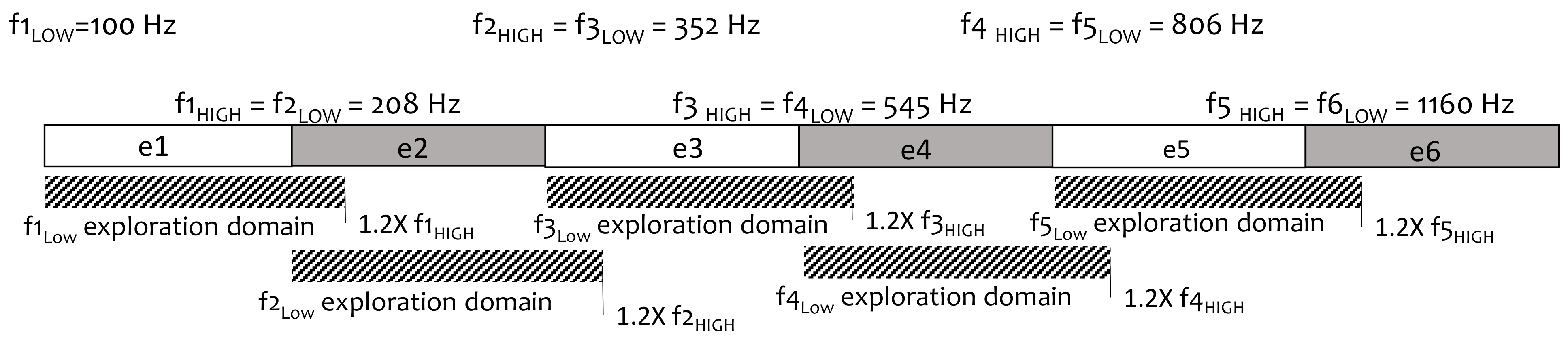
2.5. Frequency Reallocation with the Evolutionary Algorithm
- Input default settings to define the boundaries of the exploration space: exploration domain for each band was set at the lower limit of the same band (fLOW) to 1.2 times the upper limit (1.2 × fHIGH);
- Random generation of an initial population in the range allowed for each electrode: 4 parents (i.e., 4 fMAPs P1, P2, P3, P4);
- Evaluation of P1 to P4 by speech recognition in noise. Each fMAP obtains a score: SP1, SP2, SP3, SP4;
- Input SP1 to 4;
- Evolutionary loop, until stop-criteria (number of generations = 3 in our study):
- Generation of children (3 individuals, first loop: C1, C2, C3);
- Selection of 2 individuals among the previous generation by tournament: Two individuals of the previous generation are randomly selected; the one with the highest probability is chosen. The previous process is repeated. In this way, two individuals are finally selected;
- Crossover: combining electrode settings from 2 parent fMAPs to obtain a child;
- Gaussian mutation: mutations can be applied to fLOW and fHIGH with a probability Pm in the predefined range;
- Evaluation of the 3 children by WRS yielding scores SCn (first loop: SC1, SC2, SC3);
- Input SCn;
- Selection of 4 individuals with the highest WRS among all generated individuals (for the first loop: 7 fMAPS, P1 to P4, and C1 to C3).
- Output: The best fMAP (highest WRS) obtained during the evolutionary process.
2.6. Fitting Software Programs
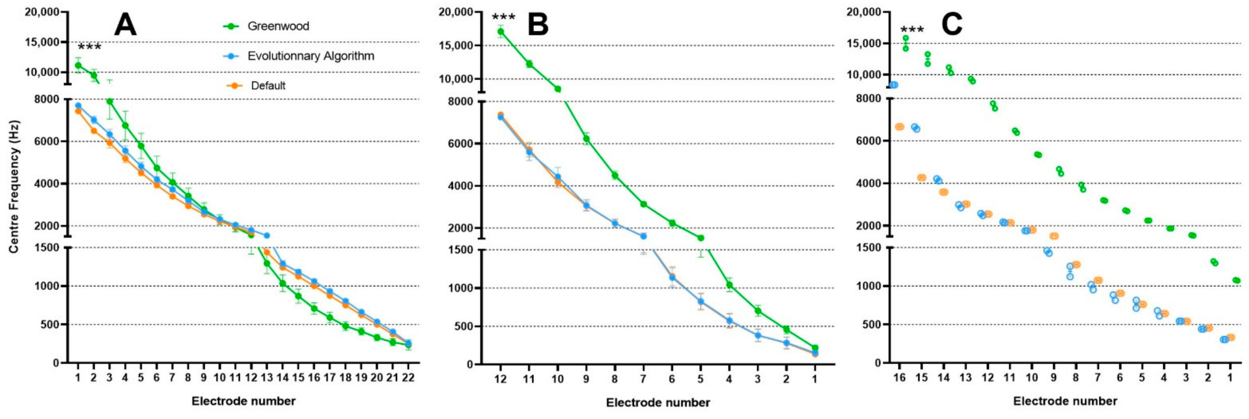
2.7. Determination of Greenwood Frequency MAP in Individual Cochleae
2.8. Statistics
3. Results
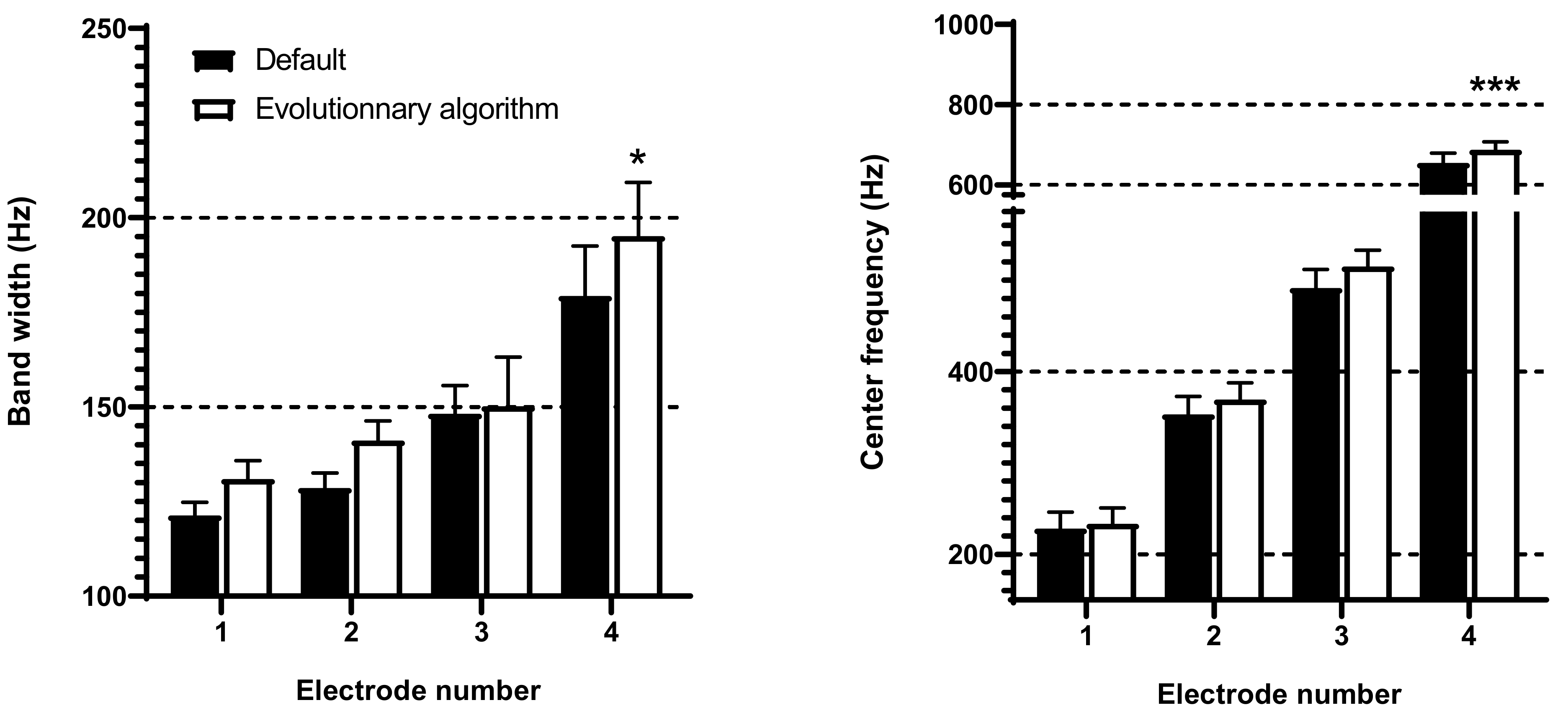
3.1. Frequency Band Adjustments with Evolutionary Algorithm
3.2. Audiometry
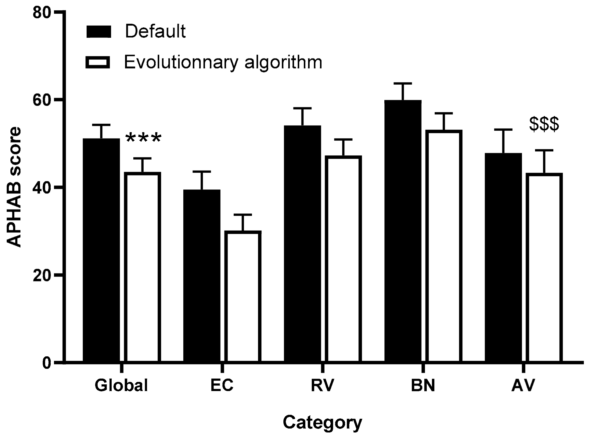
3.3. APHAB Questionnaire
3.4. HISQUI Questionnaire
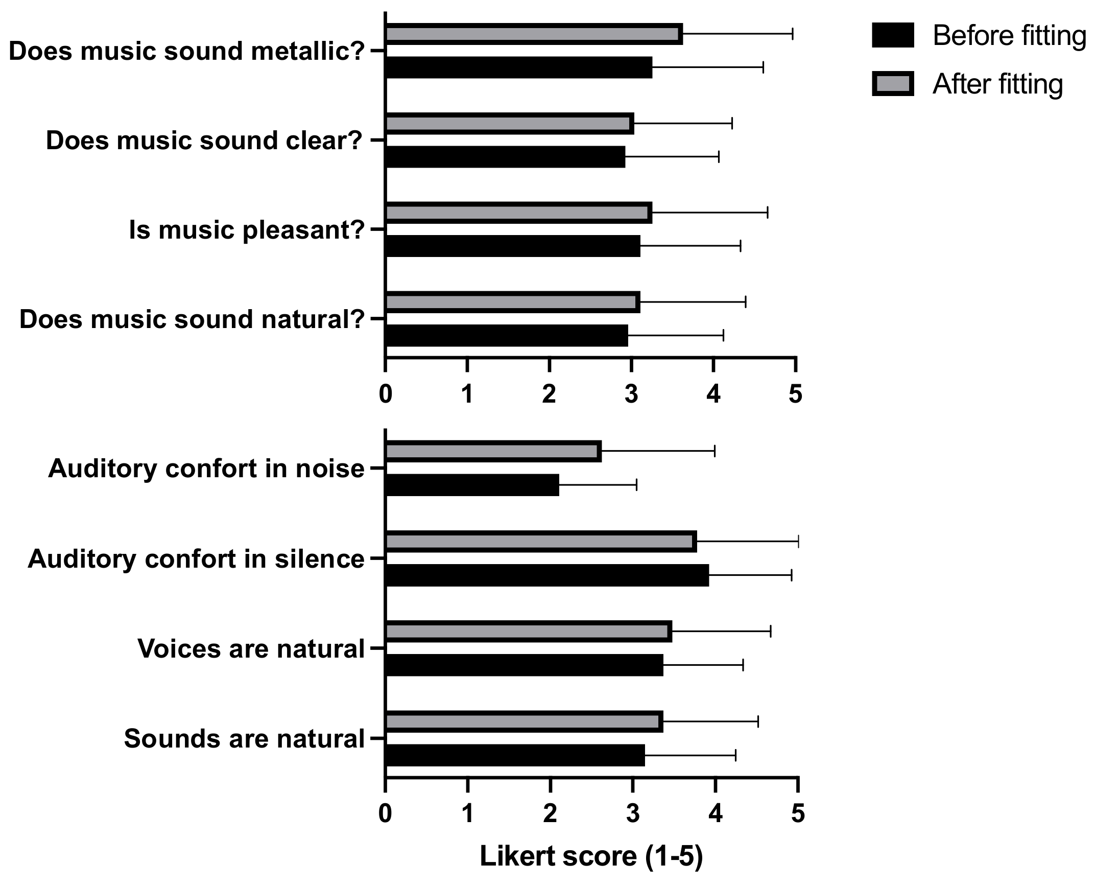
3.5. Global Evaluation of the Sound Quality and Music Perception
4. Discussion
5. Conclusions
Author Contributions
Funding
Institutional Review Board Statement
Informed Consent Statement
Acknowledgments
Conflicts of Interest
Appendix A

| e# | Initial fLOW | Initial fHIGH | Final fLOW | Final fHIGH | Initial BW | Final BW | Initial CF | Final CF |
|---|---|---|---|---|---|---|---|---|
| Patient 1 | ||||||||
| 1 | 100 | 208 | 100 | 195 | 108 | 95 | 154 | 147.5 |
| 2 | 208 | 352 | 195 | 332 | 144 | 137 | 280 | 263.5 |
| 3 | 352 | 545 | 332 | 484 | 193 | 152 | 448.5 | 408 |
| 4 | 545 | 806 | 484 | 655 | 261 | 171 | 675.5 | 569.5 |
| 5 | 806 | 1160 | 655 | 984 | 354 | 329 | 983 | 819.5 |
| 6 | 1160 | 1643 | 984 | 1619 | 483 | 635 | 1401.5 | 1301.5 |
| 7 | 1643 | 2303 | 1619 | 1917 | 660 | 298 | 1973 | 1768 |
| 8 | 2303 | 3208 | 1917 | 3048 | 905 | 1131 | 2755.5 | 2482.5 |
| 9 | 3208 | 4450 | 3048 | 4069 | 1242 | 1021 | 3829 | 3558.5 |
| 10 | 4450 | 6155 | 4069 | 6076 | 1705 | 2007 | 5302.5 | 5072.5 |
| 11 | 6155 | 8500 | 6076 | 8500 | 2345 | 2424 | 7327.5 | 7288 |
| 12 | - | - | - | - | - | - | - | - |
| Patient 2 | ||||||||
| 1 | 100 | 208 | 100 | 193 | 108 | 93 | 154 | 146.5 |
| 2 | 208 | 352 | 193 | 284 | 144 | 91 | 280 | 238.5 |
| 3 | 352 | 545 | 284 | 528 | 193 | 244 | 448.5 | 406 |
| 4 | 545 | 806 | 528 | 795 | 261 | 267 | 675.5 | 661.5 |
| 5 | 806 | 1160 | 795 | 1085 | 354 | 290 | 983 | 940 |
| 6 | 1160 | 1643 | 1085 | 1563 | 483 | 478 | 1401.5 | 1324 |
| 7 | 1643 | 2303 | 1563 | 2184 | 660 | 621 | 1973 | 1873.5 |
| 8 | 2303 | 3208 | 2184 | 2811 | 905 | 627 | 2755.5 | 2497.5 |
| 9 | 3208 | 4450 | 2811 | 4143 | 1242 | 1332 | 3829 | 3477 |
| 10 | 4450 | 6155 | 4143 | 5134 | 1705 | 991 | 5302.5 | 4638.5 |
| 11 | 6155 | 8500 | 5134 | 8500 | 2345 | 3366 | 7327.5 | 6817 |
| 12 | - | - | - | - | - | - | - | - |
| Patient 3 | ||||||||
| 1 | 188 | 313 | 188 | 298 | 125 | 110 | 250.5 | 243 |
| 2 | 313 | 438 | 298 | 409 | 125 | 111 | 375.5 | 353.5 |
| 3 | 438 | 563 | 409 | 471 | 125 | 62 | 500.5 | 440 |
| 4 | 563 | 688 | 471 | 617 | 125 | 146 | 625.5 | 544 |
| 5 | 688 | 813 | 617 | 722 | 125 | 105 | 750.5 | 669.5 |
| 6 | 813 | 938 | 722 | 871 | 125 | 149 | 875.5 | 796.5 |
| 7 | 938 | 1063 | 871 | 1001 | 125 | 130 | 1000.5 | 936 |
| 8 | 1063 | 1188 | 1001 | 1067 | 125 | 66 | 1125.5 | 1034 |
| 9 | 1188 | 1313 | 1067 | 1129 | 125 | 62 | 1250.5 | 1098 |
| 10 | 1313 | 1563 | 1129 | 1462 | 250 | 333 | 1438 | 1295.5 |
| 11 | 1563 | 1813 | 1462 | 1669 | 250 | 207 | 1688 | 1565.5 |
| 12 | 1813 | 2063 | 1669 | 1787 | 250 | 118 | 1938 | 1728 |
| 13 | 2063 | 2313 | 1787 | 1905 | 250 | 118 | 2188 | 1846 |
| 14 | 2313 | 2688 | 1905 | 2418 | 375 | 513 | 2500.5 | 2161.5 |
| 15 | 2688 | 3063 | 2418 | 3030 | 375 | 612 | 2875.5 | 2724 |
| 16 | 3063 | 3563 | 3030 | 3092 | 500 | 62 | 3313 | 3061 |
| 17 | 3563 | 4063 | 3092 | 3855 | 500 | 763 | 3813 | 3473.5 |
| 18 | 4063 | 4688 | 3855 | 4608 | 625 | 753 | 4375.5 | 4231.5 |
| 19 | 4688 | 5313 | 4608 | 5092 | 625 | 484 | 5000.5 | 4850 |
| 20 | 5313 | 6063 | 5092 | 5959 | 750 | 867 | 5688 | 5525.5 |
| 21 | 6063 | 6938 | 5959 | 6460 | 875 | 501 | 6500.5 | 6209.5 |
| 22 | 6938 | 7938 | 6460 | 7938 | 1000 | 1478 | 7438 | 7199 |
| Patient 4 | ||||||||
| 1 | 188 | 313 | 220 | 368 | 125 | 148 | 250.5 | 294 |
| 2 | 313 | 438 | 368 | 462 | 125 | 94 | 375.5 | 415 |
| 3 | 438 | 563 | 462 | 605 | 125 | 143 | 500.5 | 533.5 |
| 4 | 563 | 688 | 605 | 770 | 125 | 165 | 625.5 | 687.5 |
| 5 | 688 | 813 | 770 | 832 | 125 | 62 | 750.5 | 801 |
| 6 | 813 | 938 | 832 | 999 | 125 | 167 | 875.5 | 915.5 |
| 7 | 938 | 1063 | 999 | 1175 | 125 | 176 | 1000.5 | 1087 |
| 8 | 1063 | 1188 | 1175 | 1268 | 125 | 93 | 1125.5 | 1221.5 |
| 9 | 1188 | 1313 | 1268 | 1413 | 125 | 145 | 1250.5 | 1340.5 |
| 10 | 1313 | 1563 | 1413 | 1702 | 250 | 289 | 1438 | 1557.5 |
| 11 | 1563 | 1813 | 1702 | 2001 | 250 | 299 | 1688 | 1851.5 |
| 12 | 1813 | 2063 | 2001 | 2063 | 250 | 62 | 1938 | 2032 |
| 13 | 2063 | 2313 | 2063 | 2390 | 250 | 327 | 2188 | 2226.5 |
| 14 | 2313 | 2688 | 2390 | 2772 | 375 | 382 | 2500.5 | 2581 |
| 15 | 2688 | 3063 | 2772 | 3107 | 375 | 335 | 2875.5 | 2939.5 |
| 16 | 3063 | 3563 | 3107 | 3834 | 500 | 727 | 3313 | 3470.5 |
| 17 | 3563 | 4063 | 3834 | 4274 | 500 | 440 | 3813 | 4054 |
| 18 | 4063 | 4688 | 4274 | 5033 | 625 | 759 | 4375.5 | 4653.5 |
| 19 | 4688 | 5313 | 5033 | 5580 | 625 | 547 | 5000.5 | 5306.5 |
| 20 | 5313 | 6063 | 5580 | 6532 | 750 | 952 | 5688 | 6056 |
| 21 | 6063 | 6938 | 6532 | 7734 | 875 | 1202 | 6500.5 | 7133 |
| 22 | 6938 | 7938 | 7734 | 7938 | 1000 | 204 | 7438 | 7836 |
| Patient 5 | ||||||||
| 1 | 500 | 647 | 500 | 626 | 147 | 126 | 573.5 | 563 |
| 2 | 647 | 837 | 626 | 777 | 190 | 151 | 742 | 701.5 |
| 3 | 837 | 1083 | 777 | 973 | 246 | 196 | 960 | 875 |
| 4 | 1083 | 1401 | 973 | 1166 | 318 | 193 | 1242 | 1069.5 |
| 5 | 1401 | 1812 | 1166 | 1493 | 411 | 327 | 1606.5 | 1329.5 |
| 6 | 1812 | 2345 | 1493 | 2109 | 533 | 616 | 2078.5 | 1801 |
| 7 | 2345 | 3034 | 2109 | 2614 | 689 | 505 | 2689.5 | 2361.5 |
| 8 | 3034 | 3925 | 2614 | 3337 | 891 | 723 | 3479.5 | 2975.5 |
| 9 | 3925 | 5078 | 3337 | 4687 | 1153 | 1350 | 4501.5 | 4012 |
| 10 | 5078 | 6570 | 4687 | 5877 | 1492 | 1190 | 5824 | 5282 |
| 11 | 6570 | 8500 | 5877 | 8500 | 1930 | 2623 | 7535 | 7188.5 |
| 12 | - | - | - | - | - | - | - | - |
| Patient 6 | ||||||||
| 1 | 195 | 326 | 195 | 326 | 131 | 131 | 260.5 | 260.5 |
| 2 | 326 | 456 | 326 | 456 | 130 | 130 | 391 | 391 |
| 3 | 456 | 586 | 456 | 586 | 130 | 130 | 521 | 521 |
| 4 | 586 | 716 | 586 | 716 | 130 | 130 | 651 | 651 |
| 5 | 716 | 846 | 716 | 846 | 130 | 130 | 781 | 781 |
| 6 | 846 | 977 | 846 | 977 | 131 | 131 | 911.5 | 911.5 |
| 7 | 977 | 1107 | 977 | 1107 | 130 | 130 | 1042 | 1042 |
| 8 | 1107 | 1367 | 1107 | 1237 | 260 | 130 | 1237 | 1172 |
| 9 | 1367 | 1758 | 1237 | 1628 | 391 | 391 | 1562.5 | 1432.5 |
| 10 | 1758 | 2148 | 1628 | 2018 | 390 | 390 | 1953 | 1823 |
| 11 | 2148 | 2539 | 2018 | 2409 | 391 | 391 | 2343.5 | 2213.5 |
| 12 | 2539 | 3060 | 2409 | 2930 | 521 | 521 | 2799.5 | 2669.5 |
| 13 | 3060 | 3711 | 2930 | 3581 | 651 | 651 | 3385.5 | 3255.5 |
| 14 | 3711 | 4492 | 3581 | 4492 | 781 | 911 | 4101.5 | 4036.5 |
| 15 | 4492 | 5404 | 4492 | 5534 | 912 | 1042 | 4948 | 5013 |
| 16 | 5404 | 6185 | 5534 | 6576 | 781 | 1042 | 5794.5 | 6055 |
| 17 | 6185 | 7357 | 6576 | 7617 | 1172 | 1041 | 6771 | 7096.5 |
| 18 | - | - | - | - | - | - | - | - |
| 19 | - | - | - | - | - | - | - | - |
| 20 | - | - | - | - | - | - | - | - |
| Patient 7 | ||||||||
| 1 | 188 | 313 | 188 | 261 | 125 | 73 | 250.5 | 224.5 |
| 2 | 313 | 438 | 261 | 424 | 125 | 163 | 375.5 | 342.5 |
| 3 | 438 | 563 | 424 | 555 | 125 | 131 | 500.5 | 489.5 |
| 4 | 563 | 688 | 555 | 643 | 125 | 88 | 625.5 | 599 |
| 5 | 688 | 813 | 643 | 754 | 125 | 111 | 750.5 | 698.5 |
| 6 | 813 | 938 | 754 | 871 | 125 | 117 | 875.5 | 812.5 |
| 7 | 938 | 1063 | 871 | 933 | 125 | 62 | 1000.5 | 902 |
| 8 | 1063 | 1188 | 933 | 1095 | 125 | 162 | 1125.5 | 1014 |
| 9 | 1188 | 1313 | 1095 | 1157 | 125 | 62 | 1250.5 | 1126 |
| 10 | 1313 | 1563 | 1157 | 1408 | 250 | 251 | 1438 | 1282.5 |
| 11 | 1563 | 1813 | 1408 | 1470 | 250 | 62 | 1688 | 1439 |
| 12 | 1813 | 2063 | 1470 | 1667 | 250 | 197 | 1938 | 1568.5 |
| 13 | 2063 | 2313 | 1667 | 2048 | 250 | 381 | 2188 | 1857.5 |
| 14 | 2313 | 2688 | 2048 | 2255 | 375 | 207 | 2500.5 | 2151.5 |
| 15 | 2688 | 3063 | 2255 | 2603 | 375 | 348 | 2875.5 | 2429 |
| 16 | 3063 | 3563 | 2603 | 3442 | 500 | 839 | 3313 | 3022.5 |
| 17 | 3563 | 4063 | 3442 | 3634 | 500 | 192 | 3813 | 3538 |
| 18 | 4063 | 4688 | 3634 | 4079 | 625 | 445 | 4375.5 | 3856.5 |
| 19 | 4688 | 5313 | 4079 | 5133 | 625 | 1054 | 5000.5 | 4606 |
| 20 | 5313 | 6063 | 5133 | 5614 | 750 | 481 | 5688 | 5373.5 |
| 21 | 6063 | 6938 | 5614 | 6266 | 875 | 652 | 6500.5 | 5940 |
| 22 | 6938 | 7938 | 6266 | 7938 | 1000 | 1672 | 7438 | 7102 |
| Patient 8 | ||||||||
| 1 | 250 | 416 | 238 | 374 | 166 | 136 | 333 | 306 |
| 2 | 416 | 494 | 374 | 510 | 78 | 136 | 455 | 442 |
| 3 | 494 | 587 | 510 | 578 | 93 | 68 | 540.5 | 544 |
| 4 | 587 | 697 | 578 | 782 | 110 | 204 | 642 | 680 |
| 5 | 697 | 828 | 782 | 850 | 131 | 68 | 762.5 | 816 |
| 6 | 828 | 983 | 850 | 918 | 155 | 68 | 905.5 | 884 |
| 7 | 983 | 1168 | 918 | 1121 | 185 | 203 | 1075.5 | 1019.5 |
| 8 | 1168 | 1387 | 1121 | 1393 | 219 | 272 | 1277.5 | 1257 |
| 9 | 1387 | 1648 | 1393 | 1529 | 261 | 136 | 1517.5 | 1461 |
| 10 | 1648 | 1958 | 1529 | 2005 | 310 | 476 | 1803 | 1767 |
| 11 | 1958 | 2326 | 2005 | 2345 | 368 | 340 | 2142 | 2175 |
| 12 | 2326 | 2762 | 2345 | 2821 | 436 | 476 | 2544 | 2583 |
| 13 | 2762 | 3281 | 2821 | 3161 | 519 | 340 | 3021.5 | 2991 |
| 14 | 3281 | 3858 | 3161 | 5064 | 577 | 1903 | 3569.5 | 4112.5 |
| 15 | 3858 | 4630 | 5064 | 8054 | 772 | 2990 | 4244 | 6559 |
| 16 | 4630 | 8700 | 8054 | 8700 | 4070 | 646 | 6665 | 8377 |
| Patient 9 | ||||||||
| 1 | 250 | 416 | 238 | 374 | 166 | 136 | 333 | 306 |
| 2 | 416 | 494 | 374 | 510 | 78 | 136 | 455 | 442 |
| 3 | 494 | 587 | 510 | 578 | 93 | 68 | 540.5 | 544 |
| 4 | 587 | 697 | 578 | 646 | 110 | 68 | 642 | 612 |
| 5 | 697 | 828 | 646 | 782 | 131 | 136 | 762.5 | 714 |
| 6 | 828 | 983 | 782 | 850 | 155 | 68 | 905.5 | 816 |
| 7 | 983 | 1168 | 850 | 1054 | 185 | 204 | 1075.5 | 952 |
| 8 | 1168 | 1387 | 1054 | 1189 | 219 | 135 | 1277.5 | 1121.5 |
| 9 | 1387 | 1648 | 1189 | 1665 | 261 | 476 | 1517.5 | 1427 |
| 10 | 1648 | 1958 | 1665 | 1869 | 310 | 204 | 1803 | 1767 |
| 11 | 1958 | 2326 | 1869 | 2413 | 368 | 544 | 2142 | 2141 |
| 12 | 2326 | 2762 | 2413 | 2549 | 436 | 136 | 2544 | 2481 |
| 13 | 2762 | 3281 | 2549 | 3161 | 519 | 612 | 3021.5 | 2855 |
| 14 | 3281 | 3858 | 3161 | 5268 | 577 | 2107 | 3569.5 | 4214.5 |
| 15 | 3858 | 4630 | 5268 | 8054 | 772 | 2786 | 4244 | 6661 |
| 16 | 4630 | 8700 | 8054 | 8700 | 4070 | 646 | 6665 | 8377 |
| Patient 10 | ||||||||
| 1 | 188 | 313 | 188 | 354 | 125 | 166 | 250.5 | 271 |
| 2 | 313 | 438 | 354 | 448 | 125 | 94 | 375.5 | 401 |
| 3 | 438 | 563 | 448 | 658 | 125 | 210 | 500.5 | 553 |
| 4 | 563 | 688 | 658 | 816 | 125 | 158 | 625.5 | 737 |
| 5 | 688 | 813 | 816 | 927 | 125 | 111 | 750.5 | 871.5 |
| 6 | 813 | 938 | 927 | 1080 | 125 | 153 | 875.5 | 1003.5 |
| 7 | 938 | 1063 | 1080 | 1158 | 125 | 78 | 1000.5 | 1119 |
| 8 | - | - | - | - | - | - | - | - |
| 9 | 1068 | 1188 | 1158 | 1220 | 120 | 62 | 1128 | 1189 |
| 10 | 1188 | 1438 | 1220 | 1480 | 250 | 260 | 1313 | 1350 |
| 11 | 1438 | 1688 | 1480 | 1775 | 250 | 295 | 1563 | 1627.5 |
| 12 | 1688 | 1938 | 1775 | 2160 | 250 | 385 | 1813 | 1967.5 |
| 13 | 1938 | 2188 | 2160 | 2299 | 250 | 139 | 2063 | 2229.5 |
| 14 | 2188 | 2563 | 2299 | 2997 | 375 | 698 | 2375.5 | 2648 |
| 15 | 2563 | 2938 | 2997 | 3081 | 375 | 84 | 2750.5 | 3039 |
| 16 | 2938 | 3438 | 3081 | 4077 | 500 | 996 | 3188 | 3579 |
| 17 | 3438 | 3938 | 4077 | 4197 | 500 | 120 | 3688 | 4137 |
| 18 | 3938 | 4563 | 4197 | 4964 | 625 | 767 | 4250.5 | 4580.5 |
| 19 | 4563 | 5313 | 4964 | 5762 | 750 | 798 | 4938 | 5363 |
| 20 | 5313 | 6063 | 5762 | 6809 | 750 | 1047 | 5688 | 6285.5 |
| 21 | 6063 | 6938 | 6809 | 7702 | 875 | 893 | 6500.5 | 7255.5 |
| 22 | 6938 | 7938 | 7702 | 7938 | 1000 | 236 | 7438 | 7820 |
| Patient 11 | ||||||||
| 1 | 188 | 313 | 188 | 368 | 125 | 180 | 250.5 | 278 |
| 2 | 313 | 438 | 368 | 509 | 125 | 141 | 375.5 | 438,5 |
| 3 | 438 | 563 | 509 | 584 | 125 | 75 | 500.5 | 546.5 |
| 4 | 563 | 688 | 584 | 747 | 125 | 163 | 625.5 | 665.5 |
| 5 | 688 | 813 | 747 | 816 | 125 | 69 | 750.5 | 781.5 |
| 6 | 813 | 938 | 816 | 995 | 125 | 179 | 875.5 | 905.5 |
| 7 | 938 | 1063 | 995 | 1127 | 125 | 132 | 1000.5 | 1061 |
| 8 | 1063 | 1188 | 1127 | 1226 | 125 | 99 | 1125.5 | 1176.5 |
| 9 | 1188 | 1313 | 1226 | 1313 | 125 | 87 | 1250.5 | 1269.5 |
| 10 | 1313 | 1563 | 1313 | 1674 | 250 | 361 | 1438 | 1493.5 |
| 11 | 1563 | 1813 | 1674 | 1847 | 250 | 173 | 1688 | 1760.5 |
| 12 | 1813 | 2063 | 1847 | 2310 | 250 | 463 | 1938 | 2078.5 |
| 13 | 2063 | 2313 | 2310 | 2531 | 250 | 221 | 2188 | 2420.5 |
| 14 | 2313 | 2688 | 2531 | 3079 | 375 | 548 | 2500.5 | 2805 |
| 15 | 2688 | 3063 | 3079 | 3494 | 375 | 415 | 2875.5 | 3286.5 |
| 16 | 3063 | 3563 | 3494 | 4018 | 500 | 524 | 3313 | 3756 |
| 17 | 3563 | 4063 | 4018 | 4090 | 500 | 72 | 3813 | 4054 |
| 18 | 4063 | 4688 | 4090 | 4752 | 625 | 662 | 4375.5 | 4421 |
| 19 | 4688 | 5313 | 4752 | 5611 | 625 | 859 | 5000.5 | 5181.5 |
| 20 | 5313 | 6063 | 5611 | 6706 | 750 | 1095 | 5688 | 6158.5 |
| 21 | 6063 | 6938 | 6706 | 7846 | 875 | 1140 | 6500.5 | 7276 |
| 22 | 6938 | 7938 | 7846 | 7938 | 1000 | 92 | 7438 | 7892 |
| Patient 12 | ||||||||
| 1 | 70 | 170 | 70 | 170 | 100 | 100 | 120 | 120 |
| 2 | 170 | 300 | 170 | 325 | 130 | 155 | 235 | 247.5 |
| 3 | 300 | 469 | 325 | 487 | 169 | 162 | 384.5 | 406 |
| 4 | 469 | 690 | 487 | 702 | 221 | 215 | 579.5 | 594.5 |
| 5 | 690 | 982 | 702 | 1058 | 292 | 356 | 836 | 880 |
| 6 | 982 | 1368 | 1058 | 1453 | 386 | 395 | 1175 | 1255.5 |
| 7 | 1368 | 1881 | 1453 | 1919 | 513 | 466 | 1624.5 | 1686 |
| 8 | 1881 | 2564 | 1919 | 3076 | 683 | 1157 | 2222.5 | 2497.5 |
| 9 | 2564 | 3475 | 3076 | 3705 | 911 | 629 | 3019.5 | 3390.5 |
| 10 | 3475 | 4693 | 3705 | 4971 | 1218 | 1266 | 4084 | 4338 |
| 11 | 4693 | 6321 | 4971 | 6560 | 1628 | 1589 | 5507 | 5765.5 |
| 12 | 6321 | 8500 | 6560 | 8500 | 2179 | 1940 | 7410.5 | 7530 |
| Patient 13 | ||||||||
| 1 | 188 | 313 | 188 | 358 | 125 | 170 | 250.5 | 273 |
| 2 | 313 | 438 | 358 | 493 | 125 | 135 | 375.5 | 425.5 |
| 3 | 438 | 563 | 493 | 584 | 125 | 91 | 500.5 | 538.5 |
| 4 | 563 | 688 | 584 | 748 | 125 | 164 | 625.5 | 666 |
| 5 | 688 | 813 | 748 | 894 | 125 | 146 | 750.5 | 821 |
| 6 | 813 | 938 | 894 | 956 | 125 | 62 | 875.5 | 925 |
| 7 | 938 | 1063 | 856 | 1138 | 125 | 282 | 1000.5 | 997 |
| 8 | 1063 | 1188 | 1138 | 1318 | 125 | 180 | 1125.5 | 1228 |
| 9 | 1188 | 1313 | 1318 | 1541 | 125 | 223 | 1250.5 | 1429.5 |
| 10 | 1313 | 1563 | 1541 | 1808 | 250 | 267 | 1438 | 1674.5 |
| 11 | 1563 | 1813 | 1808 | 1870 | 250 | 62 | 1688 | 1839 |
| 12 | 1813 | 2063 | 1870 | 2373 | 250 | 503 | 1938 | 2121.5 |
| 13 | 2063 | 2313 | 2373 | 2490 | 250 | 117 | 2188 | 2431.5 |
| 14 | 2313 | 2688 | 2490 | 2793 | 375 | 303 | 2500.5 | 2641.5 |
| 15 | 2688 | 3063 | 2793 | 3216 | 375 | 423 | 2875.5 | 3004.5 |
| 16 | 3063 | 3563 | 3216 | 4002 | 500 | 786 | 3313 | 3609 |
| 17 | 3563 | 4063 | 4002 | 4447 | 500 | 445 | 3813 | 4224.5 |
| 18 | 4063 | 4688 | 4447 | 5017 | 625 | 570 | 4375.5 | 4732 |
| 19 | 4688 | 5313 | 5017 | 6196 | 625 | 1179 | 5000.5 | 5606.5 |
| 20 | 5313 | 6063 | 6196 | 6827 | 750 | 631 | 5688 | 6511.5 |
| 21 | 6063 | 6938 | 6827 | 7654 | 875 | 827 | 6500.5 | 7240.5 |
| 22 | 6938 | 7938 | 7654 | 7938 | 1000 | 284 | 7438 | 7796 |
| Patient 14 | ||||||||
| 1 | 188 | 313 | 188 | 315 | 125 | 127 | 250.5 | 251.5 |
| 2 | 313 | 438 | 315 | 512 | 125 | 197 | 375.5 | 413.5 |
| 3 | 438 | 563 | 512 | 688 | 125 | 176 | 500.5 | 600 |
| 4 | 563 | 688 | 688 | 761 | 125 | 73 | 625.5 | 724.5 |
| 5 | 688 | 813 | 761 | 936 | 125 | 175 | 750.5 | 848.5 |
| 6 | 813 | 938 | 936 | 1077 | 125 | 141 | 875.5 | 1006.5 |
| 7 | 938 | 1063 | 1077 | 1146 | 125 | 69 | 1000.5 | 1111.5 |
| 8 | 1063 | 1188 | 1146 | 1296 | 125 | 150 | 1125.5 | 1221 |
| 9 | 1188 | 1313 | 1296 | 1358 | 125 | 62 | 1250.5 | 1327 |
| 10 | 1313 | 1563 | 1358 | 1762 | 250 | 404 | 1438 | 1560 |
| 11 | 1563 | 1813 | 1762 | 1824 | 250 | 62 | 1688 | 1793 |
| 12 | 1813 | 2063 | 1824 | 2177 | 250 | 353 | 1938 | 2000.5 |
| 13 | 2063 | 2313 | 2177 | 2334 | 250 | 157 | 2188 | 2255.5 |
| 14 | 2313 | 2688 | 2334 | 2740 | 375 | 406 | 2500.5 | 2537 |
| 15 | 2688 | 3063 | 2740 | 3567 | 375 | 827 | 2875.5 | 3153.5 |
| 16 | 3063 | 3563 | 3567 | 4058 | 500 | 491 | 3313 | 3812.5 |
| 17 | 3563 | 4063 | 4058 | 4320 | 500 | 262 | 3813 | 4189 |
| 18 | 4063 | 4688 | 4320 | 5349 | 625 | 1029 | 4375.5 | 4834.5 |
| 19 | 4688 | 5313 | 5349 | 5579 | 625 | 230 | 5000.5 | 5464 |
| 20 | 5313 | 6063 | 5579 | 6595 | 750 | 1016 | 5688 | 6087 |
| 21 | 6063 | 6938 | 6595 | 7467 | 875 | 872 | 6500.5 | 7031 |
| 22 | 6938 | 7938 | 7467 | 7938 | 1000 | 471 | 7438 | 7702.5 |
| Patient 15 | ||||||||
| 1 | 70 | 170 | 70 | 197 | 100 | 127 | 120 | 133.5 |
| 2 | 170 | 300 | 197 | 354 | 130 | 157 | 235 | 275,5 |
| 3 | 300 | 469 | 354 | 480 | 169 | 126 | 384.5 | 417 |
| 4 | 469 | 690 | 480 | 816 | 221 | 336 | 579.5 | 648 |
| 5 | 690 | 982 | 816 | 1105 | 292 | 289 | 836 | 960.5 |
| 6 | 982 | 1368 | 1105 | 1394 | 386 | 289 | 1175 | 1249.5 |
| 7 | 1368 | 1881 | 1394 | 1985 | 513 | 591 | 1624.5 | 1689.5 |
| 8 | 1881 | 2564 | 1985 | 2805 | 683 | 820 | 2222.5 | 2395 |
| 9 | 2564 | 3475 | 2805 | 3965 | 911 | 1160 | 3019.5 | 3385 |
| 10 | 3475 | 4693 | 3965 | 7722 | 1218 | 3757 | 4084 | 5843.5 |
| 11 | 4693 | 6321 | 4722 | 6671 | 1628 | 1949 | 5507 | 5696.5 |
| 12 | 6321 | 8500 | 6671 | 8500 | 2179 | 1829 | 7410.5 | 7585.5 |
| Patient 16 | ||||||||
| 1 | 100 | 221 | 100 | 244 | 121 | 144 | 160.5 | 172 |
| 2 | 221 | 386 | 244 | 409 | 165 | 165 | 303.5 | 326.5 |
| 3 | 386 | 615 | 409 | 728 | 229 | 319 | 500.5 | 568.5 |
| 4 | 615 | 935 | 728 | 1015 | 320 | 287 | 775 | 871.5 |
| 5 | 935 | 1383 | 1015 | 1450 | 448 | 435 | 1159 | 1232.5 |
| 6 | 1383 | 2014 | 1450 | 2284 | 631 | 834 | 1698.5 | 1867 |
| 7 | 2014 | 2906 | 2284 | 3475 | 892 | 1191 | 2460 | 2879.5 |
| 8 | 2906 | 4169 | 3475 | 4569 | 1263 | 1094 | 3537.5 | 4022 |
| 9 | 4169 | 5959 | 4569 | 6309 | 1790 | 1740 | 5064 | 5439 |
| 10 | 5959 | 8500 | 6312 | 8500 | 2541 | 2188 | 7229.5 | 7406 |
| 11 | - | - | - | - | - | - | - | - |
| 12 | - | - | - | - | - | - | - | - |
| Patient 17 | ||||||||
| 1 | 188 | 313 | 188 | 337 | 125 | 149 | 250.5 | 262.5 |
| 2 | 313 | 438 | 337 | 501 | 125 | 164 | 375.5 | 419 |
| 3 | 438 | 563 | 501 | 563 | 125 | 62 | 500.5 | 532 |
| 4 | 563 | 688 | 563 | 751 | 125 | 188 | 625.5 | 657 |
| 5 | 688 | 813 | 751 | 882 | 125 | 131 | 750.5 | 816.5 |
| 6 | 813 | 938 | 882 | 1024 | 125 | 142 | 875.5 | 953 |
| 7 | 938 | 1063 | 1024 | 1227 | 125 | 203 | 1000.5 | 1125.5 |
| 8 | - | - | - | - | - | - | - | - |
| 9 | 1063 | 1313 | 1227 | 1397 | 250 | 170 | 1188 | 1312 |
| 10 | 1313 | 1563 | 1397 | 1808 | 250 | 411 | 1438 | 1602.5 |
| 11 | 1563 | 1813 | 1808 | 1984 | 250 | 176 | 1688 | 1896 |
| 12 | 1813 | 2188 | 1984 | 2203 | 375 | 219 | 2000.5 | 2093.5 |
| 13 | 2188 | 2563 | 2203 | 2653 | 375 | 450 | 2375.5 | 2428 |
| 14 | 2563 | 3063 | 2653 | 3505 | 500 | 852 | 2813 | 3079 |
| 15 | 3063 | 3563 | 3505 | 3900 | 500 | 395 | 3313 | 3702.5 |
| 16 | 3563 | 4188 | 3900 | 4315 | 625 | 415 | 3875.5 | 4107.5 |
| 17 | 4188 | 4938 | 4315 | 5275 | 750 | 960 | 4563 | 4795 |
| 18 | 4938 | 5813 | 5275 | 6519 | 875 | 1244 | 5375.5 | 5897 |
| 19 | 5813 | 6813 | 6519 | 7074 | 1000 | 555 | 6313 | 6796.5 |
| 20 | 6813 | 7938 | 7074 | 7938 | 1125 | 864 | 7375.5 | 7506 |
| 21 | - | - | - | - | - | - | - | - |
| 22 | - | - | - | - | - | - | - | - |
| Patient 18 | ||||||||
| 1 | 70 | 170 | 70 | 200 | 100 | 130 | 120 | 135 |
| 2 | 170 | 300 | 200 | 352 | 130 | 152 | 235 | 276 |
| 3 | 300 | 469 | 352 | 545 | 169 | 193 | 384.5 | 448.5 |
| 4 | 469 | 690 | 545 | 725 | 221 | 180 | 579.5 | 635 |
| 5 | 690 | 982 | 725 | 1098 | 292 | 373 | 836 | 911.5 |
| 6 | 982 | 1368 | 1098 | 1374 | 386 | 276 | 1175 | 1236 |
| 7 | 1368 | 1881 | 1374 | 2040 | 513 | 666 | 1624.5 | 1707 |
| 8 | 1881 | 2564 | 2040 | 2724 | 683 | 684 | 2222.5 | 2382 |
| 9 | 2564 | 3475 | 2724 | 3587 | 911 | 863 | 3019.5 | 3155.5 |
| 10 | 3475 | 4693 | 3587 | 4860 | 1218 | 1273 | 4084 | 4223.5 |
| 11 | 4693 | 6321 | 4869 | 6855 | 1628 | 1986 | 5507 | 5862 |
| 12 | 6321 | 8500 | 6855 | 8500 | 2179 | 1645 | 7410.5 | 7677.5 |
| Patient 19 | ||||||||
| 1 | 100 | 198 | 100 | 236 | 98 | 136 | 149 | 168 |
| 2 | 198 | 325 | 236 | 387 | 127 | 151 | 261.5 | 311.5 |
| 3 | 325 | 491 | 387 | 538 | 166 | 151 | 408 | 462.5 |
| 4 | 491 | 710 | 538 | 823 | 219 | 285 | 600.5 | 680.5 |
| 5 | 710 | 999 | 823 | 1147 | 289 | 324 | 854.5 | 985 |
| 6 | 999 | 1383 | 1147 | 1470 | 384 | 323 | 1191 | 1308.5 |
| 7 | 1383 | 1893 | 1470 | 2141 | 510 | 671 | 1638 | 1805.5 |
| 8 | 1893 | 2754 | 2141 | 2662 | 861 | 521 | 2323.5 | 2401.5 |
| 9 | 2574 | 3483 | 2662 | 3975 | 909 | 1313 | 3028.5 | 3318.5 |
| 10 | 3483 | 4698 | 3975 | 4727 | 1215 | 752 | 4090.5 | 4351 |
| 11 | 4698 | 6323 | 4727 | 7328 | 1625 | 2601 | 5510.5 | 6027.5 |
| 12 | 6323 | 8500 | 7328 | 8500 | 2177 | 1172 | 7411.5 | 7914 |
| Patient 20 | ||||||||
| 1 | 188 | 313 | 188 | 313 | 125 | 125 | 250.5 | 250.5 |
| 2 | 313 | 438 | 313 | 454 | 125 | 141 | 375.5 | 383.5 |
| 3 | 438 | 563 | 454 | 665 | 125 | 211 | 500.5 | 559.5 |
| 4 | 563 | 688 | 665 | 814 | 125 | 149 | 625.5 | 739.5 |
| 5 | 688 | 813 | 814 | 876 | 125 | 62 | 750.5 | 845 |
| 6 | 813 | 938 | 876 | 958 | 125 | 82 | 875.5 | 917 |
| 7 | 938 | 1063 | 958 | 1117 | 125 | 159 | 1000.5 | 1037.5 |
| 8 | 1063 | 1188 | 1117 | 1285 | 125 | 168 | 1125.5 | 1201 |
| 9 | 1188 | 1438 | 1285 | 1609 | 250 | 324 | 1313 | 1447 |
| 10 | 1438 | 1688 | 1609 | 1776 | 250 | 167 | 1563 | 1692.5 |
| 11 | 1688 | 1938 | 1776 | 2167 | 250 | 391 | 1813 | 1971.5 |
| 12 | 1938 | 2313 | 2167 | 2276 | 375 | 109 | 2125.5 | 2221.5 |
| 13 | 2313 | 2688 | 2276 | 2742 | 375 | 466 | 2500.5 | 2509 |
| 14 | 2688 | 3188 | 2742 | 2842 | 500 | 100 | 2938 | 2792 |
| 15 | 3188 | 3688 | 2842 | 2904 | 500 | 62 | 3438 | 2873 |
| 16 | 3686 | 4313 | 2904 | 4588 | 627 | 1684 | 3999.5 | 3746 |
| 17 | 4313 | 5063 | 4588 | 5492 | 750 | 904 | 4688 | 5040 |
| 18 | 5063 | 5938 | 5492 | 6541 | 875 | 1049 | 5500.5 | 6016.5 |
| 19 | 5938 | 6938 | 6541 | 7117 | 1000 | 576 | 6438 | 6829 |
| 20 | 6938 | 7935 | 7117 | 7938 | 997 | 821 | 7436.5 | 7527.5 |
| 21 | - | - | - | - | - | - | - | - |
| 22 | - | - | - | - | - | - | - | - |
| Patient 21 | ||||||||
| 1 | 188 | 313 | 188 | 313 | 125 | 125 | 250.5 | 250.5 |
| 2 | 313 | 438 | 313 | 447 | 125 | 134 | 375.5 | 380 |
| 3 | 438 | 563 | 447 | 578 | 125 | 131 | 500.5 | 512.5 |
| 4 | 563 | 688 | 578 | 781 | 125 | 203 | 625.5 | 679.5 |
| 5 | 688 | 813 | 781 | 893 | 125 | 112 | 750.5 | 837 |
| 6 | 813 | 938 | 893 | 973 | 125 | 80 | 875.5 | 933 |
| 7 | 938 | 1063 | 973 | 1161 | 125 | 188 | 1000.5 | 1067 |
| 8 | 1063 | 1188 | 1161 | 1223 | 125 | 62 | 1125.5 | 1192 |
| 9 | 1188 | 1313 | 1223 | 1327 | 125 | 104 | 1250.5 | 1275 |
| 10 | 1313 | 1563 | 1327 | 1829 | 250 | 502 | 1438 | 1578 |
| 11 | 1563 | 1813 | 1829 | 2016 | 250 | 187 | 1688 | 1922.5 |
| 12 | 1813 | 2063 | 2016 | 2446 | 250 | 430 | 1938 | 2231 |
| 13 | 2063 | 2313 | 2446 | 2599 | 250 | 153 | 2188 | 2522.5 |
| 14 | 2313 | 2688 | 2599 | 3001 | 375 | 402 | 2500.5 | 2800 |
| 15 | 2688 | 3063 | 3001 | 3562 | 375 | 561 | 2875.5 | 3281.5 |
| 16 | 3063 | 3563 | 3562 | 4189 | 500 | 627 | 3313 | 3875.5 |
| 17 | 3563 | 4063 | 4189 | 4688 | 500 | 499 | 3813 | 4438.5 |
| 18 | 4063 | 4688 | 4688 | 4866 | 625 | 178 | 4375.5 | 4777 |
| 19 | 4688 | 5313 | 4866 | 6232 | 625 | 1366 | 5000.5 | 5549 |
| 20 | 5313 | 6063 | 6232 | 6806 | 750 | 574 | 5688 | 6519 |
| 21 | 6063 | 6938 | 6806 | 7876 | 875 | 1070 | 6500.5 | 7341 |
| 22 | 6938 | 7938 | 7876 | 7938 | 1000 | 62 | 7438 | 7907 |
| Patient 22 | ||||||||
| 1 | 70 | 170 | 70 | 184 | 100 | 114 | 120 | 127 |
| 2 | 170 | 300 | 184 | 310 | 130 | 126 | 235 | 247 |
| 3 | 300 | 469 | 310 | 493 | 169 | 183 | 384.5 | 401.5 |
| 4 | 469 | 690 | 493 | 692 | 221 | 199 | 579.5 | 592.5 |
| 5 | 690 | 982 | 692 | 1163 | 292 | 471 | 836 | 927.5 |
| 6 | 982 | 1368 | 1163 | 1547 | 386 | 384 | 1175 | 1355 |
| 7 | 1368 | 1881 | 1547 | 2231 | 513 | 684 | 1624.5 | 1889 |
| 8 | 1881 | 2564 | 2231 | 2647 | 683 | 416 | 2222.5 | 2439 |
| 9 | 2564 | 3475 | 2647 | 4115 | 911 | 1468 | 3019.5 | 3381 |
| 10 | 3475 | 4693 | 4115 | 5439 | 1218 | 1324 | 4084 | 4777 |
| 11 | 4693 | 6321 | 5439 | 7050 | 1628 | 1611 | 5507 | 6244.5 |
| 12 | 6321 | 8500 | 7050 | 8500 | 2179 | 1450 | 7410.5 | 7775 |
| Patient 23 | ||||||||
| 1 | 188 | 313 | 188 | 361 | 125 | 173 | 250.5 | 274.5 |
| 2 | 313 | 438 | 361 | 507 | 125 | 146 | 375.5 | 434 |
| 3 | 438 | 563 | 507 | 584 | 125 | 77 | 500.5 | 545.5 |
| 4 | 563 | 688 | 584 | 755 | 125 | 171 | 625.5 | 669.5 |
| 5 | 688 | 813 | 755 | 885 | 125 | 130 | 750.5 | 820 |
| 6 | 813 | 938 | 885 | 1059 | 125 | 174 | 875.5 | 972 |
| 7 | 938 | 1063 | 1059 | 1214 | 125 | 155 | 1000.5 | 1136.5 |
| 8 | 1063 | 1188 | 1214 | 1310 | 125 | 96 | 1125.5 | 1262 |
| 9 | 1188 | 1313 | 1310 | 1372 | 125 | 62 | 1250.5 | 1341 |
| 10 | 1313 | 1563 | 1372 | 1738 | 250 | 366 | 1438 | 1555 |
| 11 | 1563 | 1813 | 1738 | 2050 | 250 | 312 | 1688 | 1894 |
| 12 | 1813 | 2063 | 2050 | 2130 | 250 | 80 | 1938 | 2090 |
| 13 | 2063 | 2313 | 2130 | 2368 | 250 | 238 | 2188 | 2249 |
| 14 | 2313 | 2688 | 2368 | 2956 | 375 | 588 | 2500.5 | 2662 |
| 15 | 2688 | 3063 | 2956 | 3676 | 375 | 720 | 2875.5 | 3316 |
| 16 | 3063 | 3563 | 3676 | 3805 | 500 | 129 | 3313 | 3740.5 |
| 17 | 3563 | 4063 | 3805 | 4538 | 500 | 733 | 3813 | 4171.5 |
| 18 | 4063 | 4688 | 4538 | 4975 | 625 | 437 | 4375.5 | 4756.5 |
| 19 | 4688 | 5313 | 4975 | 6196 | 625 | 1221 | 5000.5 | 5585.5 |
| 20 | 5313 | 6063 | 6196 | 6827 | 750 | 631 | 5688 | 6511.5 |
| 21 | 6063 | 6938 | 6827 | 7654 | 875 | 827 | 6500.5 | 7240.5 |
| 22 | 6938 | 7938 | 7654 | 7938 | 1000 | 284 | 7438 | 7796 |
| Patient 24 | ||||||||
| 1 | 188 | 313 | 188 | 315 | 125 | 127 | 250.5 | 251.5 |
| 2 | 313 | 438 | 315 | 517 | 125 | 202 | 375.5 | 416 |
| 3 | 438 | 563 | 517 | 641 | 125 | 124 | 500.5 | 579 |
| 4 | 563 | 688 | 641 | 781 | 125 | 140 | 625.5 | 711 |
| 5 | 688 | 813 | 781 | 942 | 125 | 161 | 750.5 | 861.5 |
| 6 | 813 | 938 | 942 | 1077 | 125 | 135 | 875.5 | 1009.5 |
| 7 | 938 | 1063 | 1077 | 1193 | 125 | 116 | 1000.5 | 1135 |
| 8 | 1063 | 1188 | 1193 | 1296 | 125 | 103 | 1125.5 | 1244.5 |
| 9 | 1188 | 1313 | 1296 | 1358 | 125 | 62 | 1250.5 | 1327 |
| 10 | 1313 | 1563 | 1358 | 1764 | 250 | 406 | 1438 | 1561 |
| 11 | 1563 | 1813 | 1764 | 1826 | 250 | 62 | 1688 | 1795 |
| 12 | 1813 | 2063 | 1826 | 2190 | 250 | 364 | 1938 | 2008 |
| 13 | 2063 | 2313 | 2190 | 2355 | 250 | 165 | 2188 | 2272.5 |
| 14 | 2313 | 2688 | 2355 | 2740 | 375 | 385 | 2500.5 | 2547.5 |
| 15 | 2688 | 3063 | 2740 | 3567 | 375 | 827 | 2875.5 | 3153.5 |
| 16 | 3063 | 3563 | 3567 | 4022 | 500 | 455 | 3313 | 3794.5 |
| 17 | 3563 | 4063 | 4022 | 4288 | 500 | 266 | 3813 | 4155 |
| 18 | 4063 | 4688 | 4288 | 5349 | 625 | 1061 | 4375.5 | 4818.5 |
| 19 | 4688 | 5313 | 5349 | 5579 | 625 | 230 | 5000.5 | 5464 |
| 20 | 5313 | 6063 | 5579 | 6537 | 750 | 958 | 5688 | 6058 |
| 21 | 6063 | 6938 | 6537 | 7467 | 875 | 930 | 6500.5 | 7002 |
| 22 | 6938 | 7938 | 7467 | 7938 | 1000 | 471 | 7438 | 7702.5 |
| Patient 25 | ||||||||
| 1 | 100 | 198 | 100 | 219 | 98 | 119 | 149 | 159.5 |
| 2 | 198 | 325 | 219 | 341 | 127 | 122 | 261.5 | 280 |
| 3 | 325 | 491 | 341 | 519 | 166 | 178 | 408 | 430 |
| 4 | 491 | 710 | 519 | 797 | 219 | 278 | 600.5 | 658 |
| 5 | 710 | 999 | 797 | 1052 | 289 | 255 | 854.5 | 924.5 |
| 6 | 999 | 1383 | 1052 | 1611 | 384 | 559 | 1191 | 1331.5 |
| 7 | 1383 | 1893 | 1611 | 2265 | 510 | 654 | 1638 | 1938 |
| 8 | 1893 | 2754 | 2265 | 2888 | 861 | 623 | 2323.5 | 2576.5 |
| 9 | 2574 | 3483 | 2888 | 3452 | 909 | 564 | 3028.5 | 3170 |
| 10 | 3483 | 4698 | 3452 | 5197 | 1215 | 1745 | 4090.5 | 4324.5 |
| 11 | 4698 | 6323 | 5197 | 7158 | 1625 | 1961 | 5510.5 | 6177.5 |
| 12 | 6323 | 8500 | 7158 | 8500 | 2177 | 1342 | 7411.5 | 7829 |
| Patient 26 | ||||||||
| 1 | 100 | 208 | 100 | 237 | 108 | 137 | 154 | 168.5 |
| 2 | 208 | 352 | 237 | 354 | 144 | 117 | 280 | 295.5 |
| 3 | 352 | 545 | 354 | 637 | 193 | 283 | 448.5 | 495.5 |
| 4 | 545 | 806 | 637 | 956 | 261 | 319 | 675.5 | 796.5 |
| 5 | 806 | 1160 | 956 | 1317 | 354 | 361 | 983 | 1136.5 |
| 6 | 1160 | 1643 | 1317 | 1891 | 483 | 574 | 1401.5 | 1604 |
| 7 | 1643 | 2303 | 1891 | 2644 | 660 | 753 | 1973 | 2267.5 |
| 8 | 2303 | 3208 | 2644 | 3459 | 905 | 815 | 2755.5 | 3051.5 |
| 9 | 3208 | 4450 | 3459 | 5033 | 1242 | 1574 | 3829 | 4246 |
| 10 | 4450 | 6155 | 5033 | 6365 | 1705 | 1332 | 5302.5 | 5699 |
| 11 | 6155 | 8500 | 6365 | 8500 | 2345 | 2135 | 7327.5 | 7432.5 |
| 12 | - | - | - | - | - | - | - | - |
| Patient 27 | ||||||||
| 1 | 188 | 313 | 188 | 328 | 125 | 140 | 250.5 | 258 |
| 2 | 313 | 438 | 328 | 490 | 125 | 162 | 375.5 | 409 |
| 3 | 438 | 563 | 490 | 599 | 125 | 109 | 500.5 | 544.5 |
| 4 | 563 | 813 | 599 | 927 | 250 | 328 | 688 | 763 |
| 5 | 813 | 1063 | 927 | 1176 | 250 | 249 | 938 | 1051.5 |
| 6 | 1063 | 1313 | 1176 | 1321 | 250 | 145 | 1188 | 1248.5 |
| 7 | 1313 | 1563 | 1321 | 1584 | 250 | 263 | 1438 | 1452.5 |
| 8 | 1563 | 1813 | 1584 | 1964 | 250 | 380 | 1688 | 1774 |
| 9 | 1813 | 2188 | 1964 | 2410 | 375 | 446 | 2000.5 | 2187 |
| 10 | 2188 | 2563 | 2410 | 2898 | 375 | 488 | 2375.5 | 2654 |
| 11 | 2563 | 3063 | 2898 | 3312 | 500 | 414 | 2813 | 3105 |
| 12 | 3063 | 3563 | 3312 | 4147 | 500 | 835 | 3313 | 3729.5 |
| 13 | 3563 | 4188 | 4147 | 4789 | 625 | 642 | 3875.5 | 4468 |
| 14 | 4188 | 4938 | 4789 | 5895 | 750 | 1106 | 4563 | 5342 |
| 15 | 4938 | 5813 | 5895 | 6430 | 875 | 535 | 5375.5 | 6162.5 |
| 16 | 5813 | 6813 | 6430 | 7256 | 1000 | 826 | 6313 | 6843 |
| 17 | 6813 | 7938 | 7256 | 7938 | 1125 | 682 | 7375.5 | 7597 |
| 18 | - | - | - | - | - | - | - | - |
| 19 | - | - | - | - | - | - | - | - |
| 20 | - | - | - | - | - | - | - | - |
| 21 | - | - | - | - | - | - | - | - |
| 22 | - | - | - | - | - | - | - | - |
Appendix B
| ID | CI Brand/Array | BML | e# | ERD | GF | DF | EAF |
|---|---|---|---|---|---|---|---|
| 1 | MEDEL/Flex 28 | 30.7 | 1 | 1.56 | 16,140.9 | 7327.5 | 7288 |
| 2 | 3.53 | 11,796.2 | 5302.5 | 5072.5 | |||
| 3 | 5.67 | 8379.27 | 3829 | 3558.5 | |||
| 4 | 7.76 | 5988.13 | 2755.5 | 2482.5 | |||
| 5 | 9.73 | 4351.89 | 1973 | 1768 | |||
| 6 | 11.78 | 3110.85 | 1401.5 | 1301.5 | |||
| 7 | 13.97 | 2160.84 | 983 | 819.5 | |||
| 8 | 16.04 | 1519.15 | 675.5 | 569.5 | |||
| 9 | 18.27 | 1026.09 | 448.5 | 408 | |||
| 10 | 20.3 | 705.461 | 280 | 263.5 | |||
| 11 | 22.41 | 464.833 | 154 | 147.5 | |||
| 2 | MEDEL/Flex 28 | 30.7 | 1 | 2.37 | 14,276.1 | 7327.5 | 6817 |
| 2 | 4.42 | 10,350.7 | 5302.5 | 4638.5 | |||
| 3 | 6.55 | 7399.64 | 3829 | 3477 | |||
| 4 | 8.45 | 5475.08 | 2755.5 | 2497.5 | |||
| 5 | 10.5 | 3945.21 | 1973 | 1873.5 | |||
| 6 | 12.5 | 2854.92 | 1401.5 | 1324 | |||
| 7 | 14.71 | 1984.74 | 983 | 940 | |||
| 8 | 16.67 | 1426.68 | 675.5 | 661.5 | |||
| 9 | 18.51 | 1036.59 | 448.5 | 406 | |||
| 10 | 20.47 | 726.911 | 280 | 238.5 | |||
| 11 | 22.32 | 509.428 | 154 | 146.5 | |||
| 3 | COCHLEAR/422 | 26.6 | 1 | 3.26 | 11,366.9 | 7438 | 7199 |
| 2 | 4.29 | 9401.1 | 6500.5 | 6209.5 | |||
| 3 | 5.09 | 8109 | 5688 | 5525.5 | |||
| 4 | 5.97 | 6888.73 | 5000.5 | 4850 | |||
| 5 | 6.85 | 5848.85 | 4375.5 | 4231.5 | |||
| 6 | 7.6 | 5084.86 | 3813 | 3473.5 | |||
| 7 | 8.4 | 4376.94 | 3313 | 3061 | |||
| 8 | 9.21 | 3757.73 | 2875.5 | 2724 | |||
| 9 | 10.02 | 3223.31 | 2500.5 | 2161.5 | |||
| 10 | 10.94 | 2704.49 | 2188 | 1846 | |||
| 11 | 11.76 | 2309.8 | 1938 | 1728 | |||
| 12 | 12.59 | 1965.93 | 1688 | 1565.5 | |||
| 13 | 13.53 | 1634.27 | 1438 | 1295.5 | |||
| 14 | 14.39 | 1376.69 | 1250.5 | 1098 | |||
| 15 | 15.06 | 1202.13 | 1125.5 | 1034 | |||
| 16 | 15.8 | 1032.51 | 1000.5 | 936 | |||
| 17 | 16.4 | 910.776 | 875.5 | 796.5 | |||
| 18 | 17.16 | 744.471 | 750.5 | 669.5 | |||
| 19 | 18.08 | 632.784 | 625.5 | 544 | |||
| 20 | 18.75 | 543.532 | 500.5 | 440 | |||
| 21 | 18.92 | 522.563 | 375.5 | 353.5 | |||
| 22 | 18.11 | 628.511 | 250.5 | 243 | |||
| 5 | MEDEL/Flex 28 | 34.2 | 1 | 2.02 | 15,503.9 | 7535 | 7188.5 |
| 2 | 4.12 | 11,483.7 | 5824 | 5282 | |||
| 3 | 6.34 | 8350.89 | 4501.5 | 4012 | |||
| 4 | 8.63 | 6000.88 | 3479.5 | 2975.5 | |||
| 5 | 10.47 | 4592.95 | 2689.5 | 2361.5 | |||
| 6 | 12.46 | 3430.86 | 2078.5 | 1801 | |||
| 7 | 14.17 | 2662.78 | 1606.5 | 1329.5 | |||
| 8 | 16.75 | 1804.41 | 1242 | 1069.5 | |||
| 9 | 18.91 | 1291.24 | 960 | 875 | |||
| 10 | 20.97 | 928.2 | 742 | 701.5 | |||
| 11 | 23.15 | 643.389 | 573.5 | 563 | |||
| 8 | AB/HiFOCUS Mid-scala | 28.6 | 1 | 2.22 | 14,160.8 | 6665 | 8377 |
| 2 | 3.32 | 11,732.9 | 4264 | 6559 | |||
| 3 | 4.1 | 10,265.3 | 3589.5 | 4112.5 | |||
| 4 | 4.9 | 8948.25 | 3021.5 | 2991 | |||
| 5 | 5.91 | 7520.72 | 2544 | 2583 | |||
| 6 | 6.86 | 6383.19 | 2142 | 2175 | |||
| 7 | 7.9 | 5330.47 | 1803 | 1767 | |||
| 8 | 8.93 | 4455.28 | 1517.5 | 1461 | |||
| 9 | 9.99 | 3700.4 | 1277.5 | 1257 | |||
| 10 | 10.8 | 3208.18 | 1075.5 | 1019.5 | |||
| 11 | 11.8 | 2686.5 | 905.5 | 884 | |||
| 12 | 12.8 | 2245.98 | 762.5 | 816 | |||
| 13 | 13.8 | 1873.97 | 642 | 680 | |||
| 14 | 14.8 | 1559.83 | 540.5 | 544 | |||
| 15 | 15.8 | 1294.56 | 455 | 442 | |||
| 16 | 16.8 | 1070.55 | 333 | 306 | |||
| 9 | AB/HiFOCUS Mid-scala | 27.5 | 1 | 1.5 | 15,849.7 | 6665 | 8377 |
| 2 | 2.5 | 13,270.6 | 4264 | 6661 | |||
| 3 | 3.46 | 11,186.7 | 3589.5 | 4214.5 | |||
| 4 | 4.46 | 9359.48 | 3021.5 | 2855 | |||
| 5 | 5.5 | 7770.99 | 2544 | 2481 | |||
| 6 | 6.5 | 6494.51 | 2142 | 2141 | |||
| 7 | 7.56 | 5365.4 | 1803 | 1767 | |||
| 8 | 8.32 | 4676.04 | 1517.5 | 1427 | |||
| 9 | 9.26 | 3941.48 | 1277.5 | 1121.5 | |||
| 10 | 10.44 | 3175.68 | 1075.5 | 952 | |||
| 11 | 11.27 | 2724.68 | 905.5 | 816 | |||
| 12 | 12.3 | 2249.21 | 762.5 | 714 | |||
| 13 | 13.28 | 1870.15 | 642 | 612 | |||
| 14 | 14.32 | 1533.28 | 540.5 | 544 | |||
| 15 | 15.08 | 1323.28 | 455 | 442 | |||
| 16 | 16.12 | 1077.81 | 333 | 306 | |||
| 11 | COCHLEAR/CI522 | 26.8 | 1 | 4.22 | 9578.87 | 7438 | 7892 |
| 2 | 4.45 | 9183.58 | 6500.5 | 7276 | |||
| 3 | 5.83 | 7127.34 | 5688 | 6158.5 | |||
| 4 | 6.35 | 6476.01 | 5000.5 | 5181.5 | |||
| 5 | 6.78 | 5981.71 | 4375.5 | 4421 | |||
| 6 | 9.29 | 3750.16 | 3813 | 4054 | |||
| 7 | 9.88 | 3356.77 | 3313 | 3756 | |||
| 8 | 10.8 | 2821.1 | 2875.5 | 3286.5 | |||
| 9 | 12.4 | 2077.21 | 2500.5 | 2805 | |||
| 10 | 13.4 | 1710.26 | 2188 | 2420.5 | |||
| 11 | 14.4 | 1403.89 | 1938 | 2078.5 | |||
| 12 | 15.2 | 1195.63 | 1688 | 1760.5 | |||
| 13 | 16.2 | 974.22 | 1438 | 1493.5 | |||
| 14 | 17.51 | 738.51 | 1250.5 | 1269.5 | |||
| 15 | 18.12 | 646.37 | 1125.5 | 1176.5 | |||
| 16 | 19.12 | 515.63 | 1000.5 | 1061 | |||
| 17 | 19.9 | 428.83 | 875.5 | 905.5 | |||
| 18 | 20.6 | 360.68 | 750.5 | 781.5 | |||
| 19 | 20.12 | 406.48 | 625.5 | 665.5 | |||
| 20 | 21.58 | 278.64 | 500.5 | 546.5 | |||
| 21 | 22.2 | 233.74 | 375.5 | 438.5 | |||
| 22 | 23.3 | 165.46 | 250.5 | 278 | |||
| 13 | COCHLEAR/CI522 | 23.2 | 1 | 1.71 | 14,434.22 | 7438 | 7796 |
| 2 | 2.42 | 12,428.74 | 6500.5 | 7240.5 | |||
| 3 | 3.39 | 10,127.08 | 5688 | 6511.5 | |||
| 4 | 4.17 | 8585.74 | 5000.5 | 5606.5 | |||
| 5 | 4.96 | 7260.21 | 4375.5 | 4732 | |||
| 6 | 5.6 | 6335.4 | 3813 | 4224.5 | |||
| 7 | 6.44 | 5294.51 | 3313 | 3609 | |||
| 8 | 7.19 | 4507.27 | 2875.5 | 3004.5 | |||
| 9 | 8.12 | 3687.41 | 2500.5 | 2641.5 | |||
| 10 | 9.15 | 2946.89 | 2188 | 2431.5 | |||
| 11 | 10.1 | 2391.39 | 1938 | 2121.5 | |||
| 12 | 11.2 | 1871.61 | 1688 | 1839 | |||
| 13 | 12 | 1561.82 | 1438 | 1674.5 | |||
| 14 | 13.1 | 1212,00 | 1250.5 | 1429.5 | |||
| 15 | 14 | 979.81 | 1125.5 | 1228 | |||
| 16 | 14.9 | 787.33 | 1000.5 | 997 | |||
| 17 | 15.7 | 644.06 | 875.5 | 925 | |||
| 18 | 16.7 | 495.5 | 750.5 | 821 | |||
| 19 | 17.3 | 420.14 | 625.5 | 666 | |||
| 20 | 18.2 | 323.39 | 500.5 | 538.5 | |||
| 21 | 19.2 | 235.16 | 375.5 | 425.5 | |||
| 22 | 20 | 176.69 | 250.5 | 273 | |||
| 14 | COCHLEAR/CI522 | 29.2 | 1 | 6.84 | 6562.82 | 7438 | 7702.5 |
| 2 | 7.92 | 5464.23 | 6500.5 | 7031 | |||
| 3 | 8.86 | 4655.58 | 5688 | 6087 | |||
| 4 | 9.64 | 4073.82 | 5000.5 | 5464 | |||
| 5 | 10.7 | 3394.54 | 4375.5 | 4834.5 | |||
| 6 | 11.7 | 2854.28 | 3813 | 4189 | |||
| 7 | 12.2 | 2615.9 | 3313 | 3812.5 | |||
| 8 | 13.1 | 2233.54 | 2875.5 | 3153.5 | |||
| 9 | 14 | 1904.12 | 2500.5 | 2537 | |||
| 10 | 14.7 | 1679.78 | 2188 | 2255.5 | |||
| 11 | 15.6 | 1427.04 | 1938 | 2000.5 | |||
| 12 | 16.7 | 1165.16 | 1688 | 1793 | |||
| 13 | 17.8 | 946.89 | 1438 | 1560 | |||
| 14 | 19 | 750.01 | 1250.5 | 1327 | |||
| 15 | 20 | 613.33 | 1125.5 | 1221 | |||
| 16 | 20.7 | 530.27 | 1000.5 | 1111.5 | |||
| 17 | 21.7 | 427.13 | 875.5 | 1006.5 | |||
| 18 | 22.6 | 347.84 | 750.5 | 848.5 | |||
| 19 | 23.4 | 286.62 | 625.5 | 724.5 | |||
| 20 | 24 | 245.74 | 500.5 | 600 | |||
| 21 | 25.1 | 180.58 | 375.5 | 413.5 | |||
| 22 | 25.9 | 140.11 | 250.5 | 251.5 | |||
| 15 | MEDEL/Flex 28 | 28.45 | 1 | 0.75 | 18,184.98 | 7410.5 | 7585.5 |
| 2 | 2.89 | 12,595.75 | 5507 | 5696.5 | |||
| 3 | 4.85 | 8985.88 | 4084 | 5843.5 | |||
| 4 | 7.07 | 6115.86 | 3019.5 | 3385 | |||
| 5 | 9.24 | 4184.53 | 2222.5 | 2395 | |||
| 6 | 11.2 | 2957.73 | 1624.5 | 1689.5 | |||
| 7 | 13.6 | 1918.25 | 1175 | 1249.5 | |||
| 8 | 16.4 | 1136.75 | 836 | 960.5 | |||
| 9 | 18.2 | 798.78 | 579.5 | 648 | |||
| 10 | 20.4 | 504.18 | 384.5 | 417 | |||
| 11 | 22.5 | 309.15 | 235 | 275.5 | |||
| 12 | 24.4 | 183.66 | 120 | 133.5 | |||
| 16 | MEDEL/Flex 28 | 28.2 | 1 | 0.87 | 17,791.38 | 7229.5 | 7406 |
| 2 | 2.39 | 13,675.99 | 5064 | 5439 | |||
| 3 | 4.68 | 9187.52 | 3537.5 | 4022 | |||
| 4 | 6.82 | 6320.85 | 2460 | 2879.5 | |||
| 5 | 8.7 | 4538.94 | 1698.5 | 1867 | |||
| 6 | 11 | 3012.26 | 1159 | 1232.5 | |||
| 7 | 13.2 | 2019.94 | 775 | 871.5 | |||
| 8 | 15.4 | 1339.44 | 500.5 | 568.5 | |||
| 9 | 18 | 805.29 | 303.5 | 326.5 | |||
| 10 | 20.2 | 506.49 | 160.5 | 172 | |||
| 11 | 22.3 | 309.32 | - | - | |||
| 12 | 24.2 | 182.85 | - | - | |||
| 17 | COCHLEAR/CI522 | 24.8 | 1 | 2.64 | 12,299.22 | - | - |
| 2 | 3.52 | 10,337.09 | - | - | |||
| 3 | 4.33 | 8805.66 | 7375.5 | 7506 | |||
| 4 | 5.19 | 7423.81 | 6313 | 6796.5 | |||
| 5 | 6.11 | 6180.84 | 5375.5 | 5897 | |||
| 6 | 6.91 | 5267.15 | 4563 | 4795 | |||
| 7 | 7.78 | 4422.64 | 3875.5 | 4107.5 | |||
| 8 | 8.67 | 3694.89 | 3313 | 3702.5 | |||
| 9 | 9.77 | 2953.55 | 2813 | 3079 | |||
| 10 | 10.8 | 2389.68 | 2375.5 | 2428 | |||
| 11 | 11.6 | 2023.53 | 2000.5 | 2093.5 | |||
| 12 | 12.6 | 1639.29 | 1688 | 1896 | |||
| 13 | 13.5 | 1352.02 | 1438 | 1602.5 | |||
| 14 | 14.5 | 1086.73 | 1188 | 1312 | |||
| 15 | 15.4 | 888.4 | - | - | |||
| 16 | 16.5 | 688.81 | 1000.5 | 1125.5 | |||
| 17 | 17.3 | 568.31 | 875.5 | 953 | |||
| 18 | 18.1 | 465.21 | 750.5 | 816.5 | |||
| 19 | 18.8 | 387.29 | 625.5 | 657 | |||
| 20 | 19.6 | 310.33 | 500.5 | 532 | |||
| 21 | 20.4 | 244.49 | 375.5 | 419 | |||
| 22 | 21.2 | 188.16 | 250.5 | 262.5 | |||
| 21 | COCHLEAR/CI522 | 28.1 | 1 | 5.48 | 7964.02 | 7438 | 7907 |
| 2 | 6.24 | 6969.87 | 6500.5 | 7341 | |||
| 3 | 7.33 | 5752.95 | 5688 | 6519 | |||
| 4 | 8.27 | 4872.01 | 5000.5 | 5549 | |||
| 5 | 9.34 | 4028.21 | 4375.5 | 4777 | |||
| 6 | 10.5 | 3272.96 | 3813 | 4438.5 | |||
| 7 | 11.3 | 2833.31 | 3313 | 3875.5 | |||
| 8 | 12.5 | 2277.55 | 2875.5 | 3281.5 | |||
| 9 | 13.6 | 1859.68 | 2500.5 | 2800 | |||
| 10 | 14.5 | 1571.98 | 2188 | 2522.5 | |||
| 11 | 15.4 | 1325.56 | 1938 | 2231 | |||
| 12 | 16.3 | 1114.49 | 1688 | 1922.5 | |||
| 13 | 17.4 | 897.19 | 1438 | 1578 | |||
| 14 | 18.2 | 763.09 | 1250.5 | 1275 | |||
| 15 | 19 | 646.23 | 1125.5 | 1192 | |||
| 16 | 19.8 | 544.4 | 1000.5 | 1067 | |||
| 17 | 20.7 | 445.41 | 875.5 | 933 | |||
| 18 | 21.6 | 360.62 | 750.5 | 837 | |||
| 19 | 22.7 | 273.33 | 625.5 | 679.5 | |||
| 20 | 23.2 | 238.79 | 500.5 | 512.5 | |||
| 21 | 24.1 | 183.65 | 375.5 | 380 | |||
| 22 | 24.9 | 141.31 | 250.5 | 250.5 | |||
| 24 | COCHLEAR/CI522 | 24.3 | 1 | 1.33 | 15,835.2 | 7438 | 7702.5 |
| 2 | 2.47 | 12,591.78 | 6500.5 | 7002 | |||
| 3 | 3.28 | 10,695.68 | 5688 | 6058 | |||
| 4 | 4.15 | 8972.32 | 5000.5 | 5464 | |||
| 5 | 4.84 | 7802.55 | 4375.5 | 4818.5 | |||
| 6 | 5.65 | 6619.38 | 3813 | 4155 | |||
| 7 | 6.53 | 5532.69 | 3313 | 3794.5 | |||
| 8 | 7.43 | 4601.63 | 2875.5 | 3153.5 | |||
| 9 | 8.44 | 3737.31 | 2500.5 | 2547.5 | |||
| 10 | 9.52 | 2986.43 | 2188 | 2272.5 | |||
| 11 | 10.3 | 2536.15 | 1938 | 2008 | |||
| 12 | 11.4 | 2008.96 | 1688 | 1795 | |||
| 13 | 12.2 | 1691.89 | 1438 | 1561 | |||
| 14 | 13.3 | 1330.67 | 1250.5 | 1327 | |||
| 15 | 14.1 | 1113.42 | 1125.5 | 1244.5 | |||
| 16 | 15.2 | 865.92 | 1000.5 | 1135 | |||
| 17 | 16 | 717.06 | 875.5 | 1009.5 | |||
| 18 | 16.8 | 590.11 | 750.5 | 861.5 | |||
| 19 | 17.7 | 469.49 | 625.5 | 711 | |||
| 20 | 18.5 | 378.97 | 500.5 | 579 | |||
| 21 | 19.4 | 292.97 | 375.5 | 416 | |||
| 22 | 20.5 | 206.76 | 250.5 | 251.5 | |||
| 26 | MEDEL/Flex 28 | 25.4 | 1 | 0 | 20,677.07 | - | - |
| 2 | 2.19 | 13,578.18 | 7327.5 | 7432.5 | |||
| 3 | 4.35 | 8951.27 | 5302.5 | 5699 | |||
| 4 | 5.24 | 7533.49 | 3829 | 4246 | |||
| 5 | 7.01 | 5336.82 | 2755.5 | 3051.5 | |||
| 6 | 9.25 | 3433.53 | 1973 | 2267.5 | |||
| 7 | 10.5 | 2675.59 | 1401.5 | 1604 | |||
| 8 | 12.1 | 1934.82 | 983 | 1136.5 | |||
| 9 | 14 | 1303.4 | 675.5 | 796.5 | |||
| 10 | 16 | 844.59 | 448.5 | 495.5 | |||
| 11 | 18.3 | 493.51 | 280 | 295.5 | |||
| 12 | 20.3 | 289.49 | 154 | 168.5 |
References
- Avan, P.; Giraudet, F.; Büki, B. Importance of Binaural Hearing. Audiol. Neurotol. 2015, 20, 3–6. [Google Scholar] [CrossRef] [PubMed]
- Kong, Y.-Y.; Stickney, G.S.; Zeng, F.-G. Speech and Melody Recognition in Binaurally Combined Acoustic and Electric Hearing. J. Acoust. Soc. Am. 2005, 117, 1351–1361. [Google Scholar] [CrossRef] [PubMed]
- Morera, C.; Manrique, M.; Ramos, A.; Garcia-Ibanez, L.; Cavalle, L.; Huarte, A.; Castillo, C.; Estrada, E. Advantages of Binaural Hearing Provided through Bimodal Stimulation via a Cochlear Implant and a Conventional Hearing Aid: A 6-Month Comparative Study. Acta Oto-Laryngol. 2005, 125, 596–606. [Google Scholar] [CrossRef] [PubMed]
- Neuman, A.C.; Waltzman, S.B.; Shapiro, W.H.; Neukam, J.D.; Zeman, A.M.; Svirsky, M.A. Self-Reported Usage, Functional Benefit, and Audiologic Characteristics of Cochlear Implant Patients Who Use a Contralateral Hearing Aid. Trends Hear. 2017, 21, 233121651769953. [Google Scholar] [CrossRef]
- Schafer, E.C.; Amlani, A.M.; Paiva, D.; Nozari, L.; Verret, S. A Meta-Analysis to Compare Speech Recognition in Noise with Bilateral Cochlear Implants and Bimodal Stimulation. Int. J. Audiol. 2011, 50, 871–880. [Google Scholar] [CrossRef]
- Van Hoesel, R.J.M. Contrasting Benefits from Contralateral Implants and Hearing Aids in Cochlear Implant Users. Hear. Res. 2012, 288, 100–113. [Google Scholar] [CrossRef]
- Zirn, S.; Arndt, S.; Aschendorff, A.; Wesarg, T. Interaural Stimulation Timing in Single Sided Deaf Cochlear Implant Users. Hear. Res. 2015, 328, 148–156. [Google Scholar] [CrossRef]
- Bernstein, J.G.W.; Goupell, M.J.; Schuchman, G.I.; Rivera, A.L.; Brungart, D.S. Having Two Ears Facilitates the Perceptual Separation of Concurrent Talkers for Bilateral and Single-Sided Deaf Cochlear Implantees. Ear Hear. 2016, 37, 289–302. [Google Scholar] [CrossRef]
- Spirrov, D.; Kludt, E.; Verschueren, E.; Büchner, A.; Francart, T. Effect of (Mis)Matched Compression Speed on Speech Recognition in Bimodal Listeners. Trends Hear 2020, 24, 2331216520948974. [Google Scholar] [CrossRef]
- Wess, J.M.; Brungart, D.S.; Bernstein, J.G.W. The Effect of Interaural Mismatches on Contralateral Unmasking With Single-Sided Vocoders. Ear Hear. 2017, 38, 374–386. [Google Scholar] [CrossRef]
- Gifford, R.H.; Dorman, M.F.; McKarns, S.A.; Spahr, A.J. Combined Electric and Contralateral Acoustic Hearing: Word and Sentence Recognition With Bimodal Hearing. J. Speech Lang. Hear. Res. 2007, 50, 835–843. [Google Scholar] [CrossRef]
- Ching, T.Y.C.; van Wanrooy, E.; Dillon, H. Binaural-Bimodal Fitting or Bilateral Implantation for Managing Severe to Profound Deafness: A Review. Trends Amplif. 2007, 11, 161–192. [Google Scholar] [CrossRef]
- Litovsky, R.Y.; Johnstone, P.M.; Godar, S.P. Benefits of Bilateral Cochlear Implants and/or Hearing Aids in Children: Beneficios de Los Implantes Cocleares Bilaterales y/o Auxiliares Auditivos En Niños. Int. J. Audiol. 2006, 45, 78–91. [Google Scholar] [CrossRef]
- Mok, M.; Grayden, D.; Dowell, R.C.; Lawrence, D. Speech Perception for Adults Who Use Hearing Aids in Conjunction With Cochlear Implants in Opposite Ears. J. Speech Lang. Hear. Res. 2006, 49, 338–351. [Google Scholar] [CrossRef]
- Kiefer, J.; Pok, M.; Adunka, O.; Stürzebecher, E.; Baumgartner, W.; Schmidt, M.; Tillein, J.; Ye, Q.; Gstoettner, W. Combined Electric and Acoustic Stimulation of the Auditory System: Results of a Clinical Study. Audiol. Neurotol. 2005, 10, 134–144. [Google Scholar] [CrossRef]
- Richard, C.; Ferrary, E.; Borel, S.; Sterkers, O.; Grayeli, A.B. Interaction Between Electric and Acoustic Cues in Diotic Condition for Speech Perception in Quiet and Noise by Cochlear Implantees. Otol. Neurotol. 2012, 33, 30–37. [Google Scholar] [CrossRef]
- Angermeier, J.; Hemmert, W.; Zirn, S. Sound Localization Bias and Error in Bimodal Listeners Improve Instantaneously When the Device Delay Mismatch Is Reduced. Trends Hear. 2021, 25, 233121652110161. [Google Scholar] [CrossRef]
- Francart, T.; McDermott, H.J. Psychophysics, Fitting, and Signal Processing for Combined Hearing Aid and Cochlear Implant Stimulation. Ear Hear. 2013, 34, 685–700. [Google Scholar] [CrossRef]
- Greenwood, D.D. A Cochlear Frequency-position Function for Several Species—29 Years Later. J. Acoust. Soc. Am. 1990, 87, 2592–2605. [Google Scholar] [CrossRef]
- Oh, Y.; Reiss, L.A.J. Binaural Pitch Fusion: Binaural Pitch Averaging in Cochlear Implant Users With Broad Binaural Fusion. Ear Hear. 2020, 41, 1450–1460. [Google Scholar] [CrossRef]
- Hartling, C.L.; Fowler, J.R.; Stark, G.N.; Glickman, B.; Eddolls, M.; Oh, Y.; Ramsey, K.; Reiss, L.A.J. Binaural Pitch Fusion in Children With Normal Hearing, Hearing Aids, and Cochlear Implants. Ear Hear. 2020, 41, 1545–1559. [Google Scholar] [CrossRef]
- Vaerenberg, B.; Smits, C.; De Ceulaer, G.; Zir, E.; Harman, S.; Jaspers, N.; Tam, Y.; Dillon, M.; Wesarg, T.; Martin-Bonniot, D.; et al. Cochlear Implant Programming: A Global Survey on the State of the Art. Sci. World J. 2014, 2014, 501738. [Google Scholar] [CrossRef]
- Veugen, L.C.E.; Chalupper, J.; Snik, A.F.M.; van Opstal, A.J.; Mens, L.H.M. Frequency-Dependent Loudness Balancing in Bimodal Cochlear Implant Users. Acta Oto-Laryngol. 2016, 136, 775–781. [Google Scholar] [CrossRef][Green Version]
- Baskent, D.; Shannon, R.V. Speech Recognition under Conditions of Frequency-Place Compression and Expansion. J. Acoust. Soc. Am. 2003, 113, 2064–2076. [Google Scholar] [CrossRef]
- Falcón-González, J.C.; Borkoski-Barreiro, S.; Limiñana-Cañal, J.M.; Ramos-Macías, Á. Reconocimiento auditivo musical y melódico en pacientes con implante coclear, mediante nuevo método de programación de asignación frecuencial. Acta Otorrinolaringol. Esp. 2014, 65, 289–296. [Google Scholar] [CrossRef]
- Maarefvand, M.; Blamey, P.J.; Marozeau, J. Pitch Matching in Bimodal Cochlear Implant Patients: Effects of Frequency, Spectral Envelope, and Level. J. Acoust. Soc. Am. 2017, 142, 2854–2865. [Google Scholar] [CrossRef]
- Arndt, S.; Laszig, R.; Aschendorff, A.; Hassepass, F.; Beck, R.; Wesarg, T. Cochlear Implant Treatment of Patients with Single-Sided Deafness or Asymmetric Hearing Loss. HNO 2017, 65, 98–108. [Google Scholar] [CrossRef]
- Williges, B.; Wesarg, T.; Jung, L.; Geven, L.I.; Radeloff, A.; Jürgens, T. Spatial Speech-in-Noise Performance in Bimodal and Single-Sided Deaf Cochlear Implant Users. Trends Hear. 2019, 23, 233121651985831. [Google Scholar] [CrossRef]
- Yoon, Y.; Liu, A.; Fu, Q.-J. Binaural Benefit for Speech Recognition with Spectral Mismatch across Ears in Simulated Electric Hearing. J. Acoust. Soc. Am. 2011, 130, EL94–EL100. [Google Scholar] [CrossRef]
- Goupell, M.J.; Stoelb, C.A.; Kan, A.; Litovsky, R.Y. The Effect of Simulated Interaural Frequency Mismatch on Speech Understanding and Spatial Release From Masking. Ear Hear. 2018, 39, 895–905. [Google Scholar] [CrossRef]
- Bernstein, J.G.W.; Stakhovskaya, O.A.; Schuchman, G.I.; Jensen, K.K.; Goupell, M.J. Interaural Time-Difference Discrimination as a Measure of Place of Stimulation for Cochlear-Implant Users with Single-Sided Deafness. Trends Hear. 2018, 22, 233121651876551. [Google Scholar] [CrossRef] [PubMed]
- Francart, T.; Wiebe, K.; Wesarg, T. Interaural Time Difference Perception with a Cochlear Implant and a Normal Ear. J. Assoc. Res. Otolaryngol. 2018, 19, 703–715. [Google Scholar] [CrossRef] [PubMed]
- Dirks, C.E.; Nelson, P.B.; Winn, M.B.; Oxenham, A.J. Sensitivity to Binaural Temporal-Envelope Beats with Single-Sided Deafness and a Cochlear Implant as a Measure of Tonotopic Match (L). J. Acoust. Soc. Am. 2020, 147, 3626. [Google Scholar] [CrossRef] [PubMed]
- Bäck, T. Evolutionary Algorithms in Theory and Practice: Evolution Strategies, Evolutionary Programming, Genetic Algorithms; Oxford University Press: Oxford, UK, 1996; ISBN 978-0-19-509971-3. [Google Scholar]
- Legrand, P.; Bourgeois-Republique, C.; Péan, V.; Harboun-Cohen, E.; Levy-Vehel, J.; Frachet, B.; Lutton, E.; Collet, P. Interactive Evolution for Cochlear Implants Fitting. Genet. Program. Evolvable Mach. 2007, 8, 319–354. [Google Scholar] [CrossRef]
- Ramesh, A.; Kambhampati, C.; Monson, J.; Drew, P. Artificial Intelligence in Medicine. Ann. R. Coll. Surg. Engl. 2004, 86, 334–338. [Google Scholar] [CrossRef]
- Govaerts, P.J.; Vaerenberg, B.; De Ceulaer, G.; Daemers, K.; De Beukelaer, C.; Schauwers, K. Development of a Software Tool Using Deterministic Logic for the Optimization of Cochlear Implant Processor Programming. Otol. Neurotol. 2010, 31, 908–918. [Google Scholar] [CrossRef]
- Meeuws, M.; Pascoal, D.; Bermejo, I.; Artaso, M.; De Ceulaer, G.; Govaerts, P.J. Computer-Assisted CI Fitting: Is the Learning Capacity of the Intelligent Agent FOX Beneficial for Speech Understanding? Cochlear Implant. Int. 2017, 18, 198–206. [Google Scholar] [CrossRef]
- Riss, D.; Hamzavi, J.-S.; Blineder, M.; Honeder, C.; Ehrenreich, I.; Kaider, A.; Baumgartner, W.-D.; Gstoettner, W.; Arnoldner, C. FS4, FS4-p, and FSP: A 4-Month Crossover Study of 3 Fine Structure Sound-Coding Strategies. Ear Hear. 2014, 35, e272–e281. [Google Scholar] [CrossRef]
- Vandali, A.E.; Whitford, L.A.; Plant, K.L.; Clark, G.M. Speech Perception as a Function of Electrical Stimulation Rate: Using the Nucleus 24 Cochlear Implant System. Ear Hear. 2000, 21, 608–624. [Google Scholar] [CrossRef]
- Wilson, B.S.; Finley, C.C.; Lawson, D.T.; Wolford, R.D.; Eddington, D.K.; Rabinowitz, W.M. Better Speech Recognition with Cochlear Implants. Nature 1991, 352, 236–238. [Google Scholar] [CrossRef]
- Bozorg-Grayeli, A.; Guevara, N.; Bebear, J.-P.; Ardoint, M.; Saaï, S.; Hoen, M.; Gnansia, D.; Romanet, P.; Lavieille, J.-P. Clinical Evaluation of the XDP Output Compression Strategy for Cochlear Implants. Eur. Arch. Otorhinolaryngol. 2016, 273, 2363–2371. [Google Scholar] [CrossRef]
- Firszt, J.B.; Holden, L.K.; Reeder, R.M.; Skinner, M.W. Speech Recognition in Cochlear Implant Recipients: Comparison of Standard HiRes and HiRes 120 Sound Processing. Otol. Neurotol. 2009, 30, 146–152. [Google Scholar] [CrossRef]
- Fournier, J.E. Vocal audiometry, its technique and results. Rev. Otoneuroophtalmol. 1950, 22, 649–656. [Google Scholar]
- Vincent, C.; Gagné, J.-P.; Leroux, T.; Clothier, A.; Larivière, M.; Dumont, F.S.; Gendron, M. French-Canadian Translation and Validation of Four Questionnaires Assessing Hearing Impairment and Handicap. Int. J. Audiol. 2017, 56, 248–259. [Google Scholar] [CrossRef]
- Amann, E.; Anderson, I. Development and Validation of a Questionnaire for Hearing Implant Users to Self-Assess Their Auditory Abilities in Everyday Communication Situations: The Hearing Implant Sound Quality Index (HISQUI19). Acta Otolaryngol. 2014, 134, 915–923. [Google Scholar] [CrossRef]
- Brockmeier, S.J.; Nopp, P.; Vischer, M.; Baumgartner, W.; Stark, T.; Schoen, F.; Mueller, J.; Braunschweig, T.; Busch, R.; Getto, M.; et al. Correlation of speech and music perception in postlingually deaf Combi 40/40+ users. In Cochlear Implants: An Update; Kubo, T., Takahashi, Y., Iwaki, T., Eds.; Kugler Publications: The Hague, The Netherlands, 2002; pp. 459–464. [Google Scholar] [CrossRef]
- Holland, J.H. Adaptation in Natural and Artificial Systems an Introductory Analysis with Applications to Biology, Control, and Artificial Intelligence; MIT Press: Cambridge, MA, USA, 1992; ISBN 978-0-262-58111-0. [Google Scholar]
- Goldberg, D.E. Genetic Algorithms in Search, Optimization, and Machine Learning; Addison-Wesley Pub. Co.: Boston, MA, USA, 1989; ISBN 978-0-201-15767-3. [Google Scholar]
- Schwefel, H.-P.; Rudolph, G. Contemporary Evolution Strategies. In Advances in Artificial Life; Morán, F., Moreno, A., Merelo, J.J., Chacón, P., Eds.; Lecture Notes in Computer Science; Springer: Berlin/Heidelberg, Germany, 1995; Volume 929, pp. 891–907. ISBN 978-3-540-59496-3. [Google Scholar]
- Schwefel, H.-P. Evolution and Optimum Seeking; Sixth-Generation Computer Technology Series; Wiley: New York, NY, USA, 1995; ISBN 978-0-471-57148-3. [Google Scholar]
- Emmerich, M.; Shir, O.M.; Wang, H. Evolution Strategies. In Handbook of Heuristics; Martí, R., Pardalos, P.M., Resende, M.G.C., Eds.; Springer International Publishing: Cham, Switzerland, 2018; pp. 89–119. ISBN 978-3-319-07123-7. [Google Scholar]
- Poli, R.; Langdon, W.B.; McPhee, N.F.; Koza, J.R. A Field Guide to Genetic Programming; Lulu Press: Morrisville, NC, USA, 2008; ISBN 978-1-4092-0073-4. [Google Scholar]
- Li, S.; Kang, L.; Zhao, X.-M. A Survey on Evolutionary Algorithm Based Hybrid Intelligence in Bioinformatics. BioMed Res. Int. 2014, 2014, 362738. [Google Scholar] [CrossRef]
- Faul, F.; Erdfelder, E.; Lang, A.-G.; Buchner, A. G*Power 3: A Flexible Statistical Power Analysis Program for the Social, Behavioral, and Biomedical Sciences. Behav. Res. Methods 2007, 39, 175–191. [Google Scholar] [CrossRef]
- Zirn, S.; Angermeier, J.; Arndt, S.; Aschendorff, A.; Wesarg, T. Reducing the Device Delay Mismatch Can Improve Sound Localization in Bimodal Cochlear Implant/Hearing-Aid Users. Trends Hear. 2019, 23, 233121651984387. [Google Scholar] [CrossRef]
- Ma, N.; Morris, S.; Kitterick, P.T. Benefits to Speech Perception in Noise From the Binaural Integration of Electric and Acoustic Signals in Simulated Unilateral Deafness. Ear Hear. 2016, 37, 248–259. [Google Scholar] [CrossRef]
- Firszt, J.B.; Holden, L.K.; Reeder, R.M.; Waltzman, S.B.; Arndt, S. Auditory Abilities after Cochlear Implantation in Adults with Unilateral Deafness: A Pilot Study. Otol. Neurotol. 2012, 33, 1339–1346. [Google Scholar] [CrossRef]
- Sladen, D.P.; Frisch, C.D.; Carlson, M.L.; Driscoll, C.L.W.; Torres, J.H.; Zeitler, D.M. Cochlear Implantation for Single-Sided Deafness: A Multicenter Study: Cochlear Implantation for SSD. Laryngoscope 2017, 127, 223–228. [Google Scholar] [CrossRef]
- Buss, E.; Dillon, M.T.; Rooth, M.A.; King, E.R.; Deres, E.J.; Buchman, C.A.; Pillsbury, H.C.; Brown, K.D. Effects of Cochlear Implantation on Binaural Hearing in Adults With Unilateral Hearing Loss. Trends Hear. 2018, 22, 233121651877117. [Google Scholar] [CrossRef] [PubMed]
- Litovsky, R.Y.; Moua, K.; Godar, S.; Kan, A.; Misurelli, S.M.; Lee, D.J. Restoration of Spatial Hearing in Adult Cochlear Implant Users with Single-Sided Deafness. Hear. Res. 2019, 372, 69–79. [Google Scholar] [CrossRef] [PubMed]
- Thompson, N.J.; Dillon, M.T.; Buss, E.; Rooth, M.A.; King, E.R.; Bucker, A.L.; McCarthy, S.A.; Deres, E.J.; O’Connell, B.P.; Pillsbury, H.C.; et al. Subjective Benefits of Bimodal Listening in Cochlear Implant Recipients with Asymmetric Hearing Loss. Otolaryngol. Head Neck Surg. 2020, 162, 933–941. [Google Scholar] [CrossRef] [PubMed]
- Grasmeder, M.L.; Verschuur, C.A.; Batty, V.B. Optimizing Frequency-to-Electrode Allocation for Individual Cochlear Implant Users. J. Acoust. Soc. Am. 2014, 136, 3313–3324. [Google Scholar] [CrossRef]
- Sridhar, D.; Stakhovskaya, O.; Leake, P.A. A Frequency-Position Function for the Human Cochlear Spiral Ganglion. Audiol. Neurotol. 2006, 11, 16–20. [Google Scholar] [CrossRef]
- Simpson, A.; McDermott, H.J.; Dowell, R.C.; Sucher, C.; Briggs, R.J.S. Comparison of Two Frequency-to-Electrode Maps for Acoustic-Electric Stimulation. Int. J. Audiol. 2009, 48, 63–73. [Google Scholar] [CrossRef]
- Moore, B.C.J. Coding of Sounds in the Auditory System and Its Relevance to Signal Processing and Coding in Cochlear Implants. Otol. Neurotol. 2003, 24, 243–254. [Google Scholar] [CrossRef]
- Henry, B.A.; McKay, C.M.; McDermott, H.J.; Clark, G.M. The Relationship between Speech Perception and Electrode Discrimination in Cochlear Implantees. J. Acoust. Soc. Am. 2000, 108, 1269. [Google Scholar] [CrossRef]
- Leigh, J.R.; Henshall, K.R.; McKay, C.M. Optimizing Frequency-to-Electrode Allocation in Cochlear Implants. J. Am. Acad. Audiol. 2004, 15, 574–584. [Google Scholar] [CrossRef]
- McKay, C.M.; Henshall, K.R. Frequency-to-Electrode Allocation and Speech Perception with Cochlear Implants. J. Acoust. Soc. Am. 2002, 111, 1036–1044. [Google Scholar] [CrossRef]
- Stakhovskaya, O.; Sridhar, D.; Bonham, B.H.; Leake, P.A. Frequency Map for the Human Cochlear Spiral Ganglion: Implications for Cochlear Implants. JARO 2007, 8, 220–233. [Google Scholar] [CrossRef]
- Vermeire, K.; Landsberger, D.M.; Van de Heyning, P.H.; Voormolen, M.; Kleine Punte, A.; Schatzer, R.; Zierhofer, C. Frequency-Place Map for Electrical Stimulation in Cochlear Implants: Change over Time. Hear. Res. 2015, 326, 8–14. [Google Scholar] [CrossRef]
- Dorman, M.F.; Spahr, T.; Gifford, R.; Loiselle, L.; McKarns, S.; Holden, T.; Skinner, M.; Finley, C. An Electric Frequency-to-Place Map for a Cochlear Implant Patient with Hearing in the Nonimplanted Ear. JARO 2007, 8, 234–240. [Google Scholar] [CrossRef]
- Tan, C.-T.; Martin, B.; Svirsky, M.A. Pitch Matching between Electrical Stimulation of a Cochlear Implant and Acoustic Stimuli Presented to a Contralateral Ear with Residual Hearing. J. Am. Acad. Audiol. 2017, 28, 187–199. [Google Scholar] [CrossRef]
- Bernstein, J.G.W.; Jensen, K.K.; Stakhovskaya, O.A.; Noble, J.H.; Hoa, M.; Kim, H.J.; Shih, R.; Kolberg, E.; Cleary, M.; Goupell, M.J. Interaural Place-of-Stimulation Mismatch Estimates Using CT Scans and Binaural Perception, But Not Pitch, Are Consistent in Cochlear-Implant Users. J. Neurosci. 2021, 41, 10161–10178. [Google Scholar] [CrossRef]
- Neher, T. Characterizing the Binaural Contribution to Speech-in-Noise Reception in Elderly Hearing-Impaired Listeners. J. Acoust. Soc. Am. 2017, 141, EL159–EL163. [Google Scholar] [CrossRef]
- Carbonell, K.M. Reliability of Individual Differences in Degraded Speech Perception. J. Acoust. Soc. Am. 2017, 142, EL461–EL466. [Google Scholar] [CrossRef]
- Carlyon, R.P.; Macherey, O.; Frijns, J.H.M.; Axon, P.R.; Kalkman, R.K.; Boyle, P.; Baguley, D.M.; Briggs, J.; Deeks, J.M.; Briaire, J.J.; et al. Pitch Comparisons between Electrical Stimulation of a Cochlear Implant and Acoustic Stimuli Presented to a Normal-Hearing Contralateral Ear. JARO 2010, 11, 625–640. [Google Scholar] [CrossRef]
- Green, T.; Faulkner, A.; Rosen, S. Frequency Selectivity of Contralateral Residual Acoustic Hearing in Bimodal Cochlear Implant Users, and Limitations on the Ability to Match the Pitch of Electric and Acoustic Stimuli. Int. J. Audiol. 2012, 51, 389–398. [Google Scholar] [CrossRef]
- Cronbach, L.J.; Warrington, W.G. Time-Limit Tests: Estimating Their Reliability and Degree of Speeding. Psychometrika 1951, 16, 167–188. [Google Scholar] [CrossRef]
- Arnoldner, C.; Kaider, A.; Hamzavi, J. The Role of Intensity Upon Pitch Perception in Cochlear Implant Recipients. Laryngoscope 2006, 116, 1760–1765. [Google Scholar] [CrossRef] [PubMed]
- Arnoldner, C.; Riss, D.; Kaider, A.; Mair, A.; Wagenblast, J.; Baumgartner, W.-D.; Gstöttner, W.; Hamzavi, J.-S. The Intensity–Pitch Relation Revisited: Monopolar Versus Bipolar Cochlear Stimulation. Laryngoscope 2008, 118, 1630–1636. [Google Scholar] [CrossRef] [PubMed]
- Neuhoff, J.G.; Wayand, J.; Kramer, G. Pitch and Loudness Interact in Auditory Displays: Can the Data Get Lost in the Map? J. Exp. Psychol. Appl. 2002, 8, 17–25. [Google Scholar] [CrossRef] [PubMed]


| ID# | Etiology | Hearing Deprivation on Implanted Ear (Years) | Implant | Coding | Contralateral Hearing Aid |
|---|---|---|---|---|---|
| 1 | Otosclerosis | 55 | MED-EL | FS4 [39] | Chili SP7, Oticon |
| 2 | Congenital | 28 | MED-EL | FS4 | Legend 1786, Beltone |
| 3 | Congenital | 38 | COCHLEAR | ACE [40] | Naida Q70-SP, Phonak |
| 4 | Ménière | 17 | COCHLEAR | ACE | Cobalt 8+, Rexton |
| 5 | Congenital | 23 | MED-EL | HDCIS [41] | Normal |
| 6 | Congenital | 43 | OTICON | Crystalis XDP [42] | Nitro 7MI SP, Siemens |
| 7 | Congenital | 34 | COCHLEAR | ACE | Ambra SP, Phonak |
| 8 | Sudden SNHL | 1 | AB | HiRes Optima [43] | Insio 5bX, Siemens |
| 9 | Idiopathic | 16 | AB | HiRes Optima | UPSmart988 GN Resound |
| 10 | Lobstein’s disease | 42 | COCHLEAR | ACE | PHONAK Naida Q50 SP |
| 11 | Congenital | 39 | COCHLEAR | ACE | Siemens Signia Orion 2312 |
| 12 | Sudden SNHL | 18 | MED-EL | FS4 | Widex Moment |
| 13 | Congenital | 20 | COCHLEAR | ACE | Siemens Pure 500 |
| 14 | Sudden SNHL | 30 | COCHLEAR | ACE | Phonak Naida V90 UP |
| 15 | Sudden SNHL | 13 | MED-EL | FS4 | Starkey Livio 2400 |
| 16 | Otosclerosis | 2 | MED-EL | FS4 | Normal |
| 17 | Otosclerosis | 7 | COCHLEAR | ACE | Phonak Audeo B50 R |
| 18 | Neurofibromatosis type 2 | 19 | MED-EL | FS4 | Phonak Naida Q70 SP |
| 19 | Chronic otitis media | 42 | MED-EL | FS4 | No hearing aid |
| 20 | Perilymphatic fistula | 2 | COCHLEAR | ACE | Siemens Rexton Strata 2 |
| 21 | Perilymphatic fistula | 9 | COCHLEAR | ACE | Normal |
| 22 | Chronic otitis media | 50 | MED-EL | FS4 | Siemens Motion XS |
| 23 | Congenital | 32 | COCHLEAR | ACE | Gn Hearing Resound Alera 7 |
| 24 | Ménière | 2 | COCHLEAR | ACE | Belton Identity 86D |
| 25 | Meningitis | 30 | MED-EL | FS4 | Siemens Signia Pure 312 |
| 26 | Ménière | 17 | MED-EL | FS4 | Starkey Resound |
| 27 | Sudden SNHL | 5 | COCHLEAR | ACE | Belton Identity 66D |
| Patient Number | Initial WRS | SNR (dB HL) | Parents | 1st Generation | 2nd Generation | 3rd Generation | Final WRS | |||||||||
|---|---|---|---|---|---|---|---|---|---|---|---|---|---|---|---|---|
| P1 | P2 | P3 | P4 | C1 | C2 | C3 | C4 | C5 | C6 | C7 | C8 | C9 | ||||
| 1 | 4 | 10 | 6 | 8 | 6 | 6 | 8 | 6 | 9 * | 6 | 7 | 7 | 7 | 6 | 7 | 9 |
| 2 | 5 | 5 | 7 | 6 | 10 * | 9 | 4 | 6 | 10 | 9 | - | - | - | - | - | 6.5 |
| 3 | 4 | 10 | 6 | 4 | 5 | 5 | 5 | 5 | 6 | 8 * | 7 | 8 | 8 | 8 | 6 | 7.5 |
| 4 | 4 | 0 | 5 | 3 | 5 | 6 | 6 * | 4 | - | - | - | - | - | - | - | 6 |
| 5 | 4 | −7 | 4 | 4 | 5 | 8 | 6 | 7 | 6 | 5 | 5 | 9 * | 7 | 6 | 8 | 8 |
| 6 | 5 | 10 | 0 | 2 | 4 | 5 | 2 | 3 | 4 | 5 | 6 * | 5 | 4 | 0 | 5 | 5 |
| 7 | 3 | 5 | 4 | 7 | 6 | 7 | 5 | 7 | 9 * | 6 | 8 | 4 | 7 | 6 | 7 | 7.5 |
| 8 | 5.5 | 5 | 7 | 5 | 6 | 7 | 4 | 5 | 5 | 7 | 5 | 6 | 7 * | 6 | 6 | 7.5 |
| 9 | 5 | 10 | 4 | 6 | 8 * | 5 | 5 | 6 | 6 | 7 | 8 | 7 | 7 | 6 | 5 | 7.5 |
| 10 | 3 | 10 | 2 | 4 | 2 | 3 | 5 | 4 | 5 | 3 | 5 | 4 | 3 | 4 | 9 * | 2 |
| 11 | 6 | 10 | 6 | 9 | 7 | 5 | 5 | 6 | 8 | 6 | 8 | 8 | 8 | 9 * | 6 | 8 |
| 12 | 6 | −5 | 5 | 4 | 3 | 5 | 7 | 6 | 7 | 4 | 4 | 7 | 4 | 5 | 8 * | 7 |
| 13 | 3 | 0 | 6 | 2 | 5 | 5 | 4 | 7 | 6 | 2 | 6 | 7 | 4 | 6 | 8 * | 7 |
| 14 | 3 | 0 | 4 | 8 * | 6 | 2 | 4 | 3 | 6 | 2 | 4 | 3 | 6 | 5 | 5 | 8 |
| 15 | 4 | −5 | 5 | 2 | 4 | 6 | 8 * | 4 | 3 | 7 | 5 | 4 | 1 | 4 | 4 | 7 |
| 16 | 4 | −10 | 5 | 4 | 1 | 2 | 3 | 4 | 6 * | 4 | 5 | 4 | 2 | 3 | 5 | 7 |
| 17 | 5 | −5 | 3 | 5 | 8 * | 3 | 4 | 4 | 5 | 1 | 3 | 7 | 3 | 3 | 2 | 7 |
| 18 | 4 | −5 | 4 | 6 * | 2 | 5 | 2 | 2 | 3 | 5 | 1 | 5 | 5 | 4 | 5 | 7 |
| 19 | 3 | −5 | 3 | 5 | 4 | 4 | 8 * | 4 | 3 | 5 | 5 | 4 | 3 | 5 | 5 | 6 |
| 20 | 5 | −10 | 1 | 1 | 1 | 1 | 7 | 7 * | 4 | 5 | 5 | 7 | 5 | 6 | 5 | 5 |
| 21 | 4 | 0 | 2 | 5 | 2 | 2 | 3 | 4 | 4 | 2 | 3 | 2 | 5 | 5 * | 4 | 3 |
| 22 | 3 | 0 | 7 * | 3 | 5 | 5 | 6 | 5 | 4 | 4 | 4 | 2 | 2 | 6 | 6 | 7 |
| 23 | 3 | 10 | 4 | 2 | 4 | 2 | 1 | 3 | 7 | 8 * | 2 | 4 | 5 | 1 | 4 | 7 |
| 24 | 5 | 0 | 3 | 5 | 7 | 3 | 3 | 2 | 4 | 3 | 4 | 6 | 7 * | 3 | 2 | 6 |
| 25 | 5 | 0 | 4 | 1 | 3 | 4 | 5 | 4 | 3 | 3 | 6 * | 4 | 4 | 1 | 1 | 3 |
| 26 | 3 | 0 | 4 | 3 | 5 | 4 | 2 | 6 | 6 | 4 | 3 | 2 | 4 | 7 * | 4 | 6 |
| 27 | 4 | −5 | 2 | 3 | 3 | 4 | 5 | 3 | 3 | 6 * | 4 | 1 | 4 | 5 | 5 | 7 |
Publisher’s Note: MDPI stays neutral with regard to jurisdictional claims in published maps and institutional affiliations. |
© 2022 by the authors. Licensee MDPI, Basel, Switzerland. This article is an open access article distributed under the terms and conditions of the Creative Commons Attribution (CC BY) license (https://creativecommons.org/licenses/by/4.0/).
Share and Cite
Saadoun, A.; Schein, A.; Péan, V.; Legrand, P.; Aho Glélé, L.S.; Bozorg Grayeli, A. Frequency Fitting Optimization Using Evolutionary Algorithm in Cochlear Implant Users with Bimodal Binaural Hearing. Brain Sci. 2022, 12, 253. https://doi.org/10.3390/brainsci12020253
Saadoun A, Schein A, Péan V, Legrand P, Aho Glélé LS, Bozorg Grayeli A. Frequency Fitting Optimization Using Evolutionary Algorithm in Cochlear Implant Users with Bimodal Binaural Hearing. Brain Sciences. 2022; 12(2):253. https://doi.org/10.3390/brainsci12020253
Chicago/Turabian StyleSaadoun, Alexis, Antoine Schein, Vincent Péan, Pierrick Legrand, Ludwig Serge Aho Glélé, and Alexis Bozorg Grayeli. 2022. "Frequency Fitting Optimization Using Evolutionary Algorithm in Cochlear Implant Users with Bimodal Binaural Hearing" Brain Sciences 12, no. 2: 253. https://doi.org/10.3390/brainsci12020253
APA StyleSaadoun, A., Schein, A., Péan, V., Legrand, P., Aho Glélé, L. S., & Bozorg Grayeli, A. (2022). Frequency Fitting Optimization Using Evolutionary Algorithm in Cochlear Implant Users with Bimodal Binaural Hearing. Brain Sciences, 12(2), 253. https://doi.org/10.3390/brainsci12020253