Article

Second Harmonic Revisited: An Analytic Quantum Approach

1
Department of Science and High Technology, University of Insubria, Via Valleggio 11, I-22100 Como, Italy
2
SISSA, Via Bonomea 265, I-34136 Trieste, Italy
3
Institute for Photonics and Nanotechnologies, CNR, Via Valleggio 11, I-22100 Como, Italy
*
Author to whom correspondence should be addressed.
Appl. Sci. 2019, 9(8), 1690; https://doi.org/10.3390/app9081690
Submission received: 29 March 2019 / Revised: 15 April 2019 / Accepted: 17 April 2019 / Published: 24 April 2019
(This article belongs to the Special Issue Quantum Optics for Fundamental Quantum Mechanics)

Abstract

:
We address the second-harmonic generation process in a quantum frame. Starting with a perturbative approach, we show that it is possible to achieve a number of analytic results, ranging from the up-conversion probability to the statistical properties of the generated light. In particular, the moments and the correlations of the photon-number distribution of the second-harmonic light generated by any initial state are retrieved. When possible, a comparison with the results achieved with the classical regime is successfully provided. The nonclassicality of some benchmark states is investigated by inspecting the corresponding autocorrelation function.

1. Introduction

Following the first observation of second-harmonic generation (SHG) by Franken et al. [1], the process has been the subject of a huge amount of theoretical and experimental investigations. The exact solution of the equation of motion for the classical field amplitudes, provided by Armstrong et al. [2], paved the way toward a formal analytic treatment of the problem. On the other hand, the quantum dynamics does not yield exact solutions, so that the quantum description of the process has been approached in a number of different ways, such as the analogy with the Dicke model [3,4] or the assumption of a factorization hypothesis on the moments of the photon number [5,6]. However, the most common strategy is the perturbative approach [7], often followed by a numeric analysis [8,9,10].
Here, we review the simplest quantum description starting from a perturbative approach to the basic interaction Hamiltonian of the process, and we find a series of analytic results on the evolution of the pump field, the SHG probability, and the transformation of the statistics. In Section 2.1, we briefly report the well-known classical description of SHG focusing on the transformation of the statistics in the cases of coherent and chaotic light. In particular, we resume the results of a previous work by us, where, by applying a semiclassical approach, we have demonstrated [11] that the second-harmonic of a fundamental beam featuring multi-mode thermal statistics exhibits a more-than-thermal, namely superthermal, statistics. In Section 2.2, we approach the quantum model. Firstly, we retrieve some general results on the generation of second-harmonic (SH) light by inspecting the perturbative evolution of both the photon-number operator and the SH state. Then, we find that, in some simple cases, the SH conversion probability converges to periodic analytic functions. Finally, supported by the comparison with the classical results and by the quantum description, we move to the analysis of the output statistics by inspecting the Glauber autocorrelation function [12] of the SH field. In particular, we analytically retrieve it for the cases of coherent, chaotic, and squeezed light.

2. Results

2.1. Classical Regime

Given an electric field E(x, t) propagating in a second-order nonlinear material, the SHG process can be described by solving Maxwell’s equations in the absence of free charges and magnetic fields. The bound charges in the material are sources of a polarization vector PNL, which, in the particular case of SHG, is given by [2]:
P NL ( ω SH ) = ε 0 χ ( 2 ) ( ω SH = 2 ω F ) : E ( ω F ) E ( ω F )
being ϵ0 the permittivity of free space and χ ( 2 ) ( ω SH = 2 ω F ) the nonlinear susceptibility tensor related to this process. From now on, we fix the geometry and the symmetries of the nonlinear crystal so that χ ( 2 ) can be assumed to be a real scalar factor [13]. In particular, we conform to the contracted notation and rename d eff χ ( 2 ) / 2 . Maxwell’s equations provide a wave equation driven by this nonlinear polarization, i.e., [2,13]:
2 E ϵ c 2 t 2 E = 1 ε 0 c 2 t 2 P NL ,
where ϵ is the dimensionless permittivity of the material and c is the speed of light in free space. We assume that the propagation of the field is along the z axis and that the angular wave number is k j = n j ω j / c , where nj is the refractive index of the material corresponding to frequency ωj, being j = F, SH.
We express the fundamental field EF and the second-harmonic field ESH as [13]:
E j ( z , t ) = A j ( z ) e i k j z i ω j t
and the nonlinear polarization as:
P NL ( z , t ) = P NL ( 1 ) ( z , t ) + P NL ( 2 ) ( z , t ) ,
where [13]
P NL ( 1 ) ( z , t ) = 4 ϵ 0 d eff A SH A F * e i ( k SH k F ) z i ω F t
P NL ( 2 ) ( z , t ) = 2 ϵ 0 d eff A F 2 e i k SH z i ω SH t .
It is common to assume the variation of the field amplitude small with respect to the field wavelength (slowly-varying-amplitude approximation), i.e.,
| z 2 A SH | | k SH z A SH | .
This assumption leads to the coupled-amplitude equations:
d A F d z = 2 i ω F d eff n F c A SH A F * exp [ i Δ k z ]
d A SH d z = i ω SH d eff n SH c A F 2 exp [ i Δ k z ]
where Δ k = 2 k F k SH is the phase mismatch. In the so-called undepleted-pump regime, we further assume that A SH ( z ) A F ( z ) z, so that A F can be assumed to be constant with z, and the only equation to be solved in the system (8)–(9) is the second one.
Hence, it is possible to retrieve the output intensity I SH = 2 n SH ϵ 0 c | A SH | 2 as [13]:
I SH ( L , ω SH ) = ω SH 2 d eff 2 L 2 2 n SH n F 2 c 3 ϵ 0 sinc 2 Δ k L 2 I F 2 ( ω F ) ,
where L is the crystal length.
Given the link between the incoming light intensity and the second-harmonic one in Equation (10), it is possible to find a relation between the two corresponding light distributions [11,14,15]. Upon writing Equation (10) as I SH ( L , ω SH ) = a f ( I F ( ω F ) ) = a I F 2 ( ω F ) , where a is a coupling constant and f ( I F ) is an invertible function ( I F > 0 ), the second-harmonic light distribution G ( I SH ) can be expressed as a function of the incoming one, P ( I F ) ,
G ( I SH ) = P ( f 1 ( I SH ) ) d f ( I F ) d I F f 1 ( I SH ) 1 ,
which implies:
G ( I SH ) = P ( I SH / a ) 2 a I SH .

2.1.1. Coherent State

If the second-harmonic crystal is pumped with a coherent state, P ( I F ) is a delta distribution:
P ( I F ) = δ ( I F I 0 ) ,
where I0 is the intensity of the fundamental field at the crystal entrance. The second-harmonic distribution reads:
G ( I SH ) = 1 2 a I SH δ I SH a I 0 .
By applying the properties of the delta distribution, Equation (14) takes the more familiar form:
G ( I SH ) = δ ( I SH a I 0 2 ) .
Therefore, the second-harmonic distribution in this case is the same as the input light distribution, which means that the detected-photon statistics of the incoming light and that of the second harmonic are both Poissonian.

2.1.2. Multithermal State

If the input light is a multithermal radiation with μ number of equally-populated modes, i.e.,
P ( I F ) = 1 ( μ 1 ) ! μ I F μ I F μ 1 exp μ I F I F ,
we find that the second-harmonic light displays superthermal fluctuations, according to:
G ( I SH ) = 1 ( μ 1 ) ! μ I F μ I SH μ / 2 1 2 a μ / 2 exp μ I F a I SH .
The first and second moments of the distribution in Equation (17) are:
I SH = μ + 1 μ a I F 2
I SH 2 = ( μ + 3 ) ( μ + 2 ) ( μ + 1 ) μ 3 a 2 I F 4
and the variance reads:
Δ I SH 2 = 2 ( 2 μ + 3 ) ( μ + 1 ) μ 3 a 2 I F 4 .
Mandel’s formula [16] provides the detected-photon distribution for the second-harmonic field [11], that is:
g ( m ) = Γ [ 1 / 2 + m + μ / 2 ] Γ [ m + μ / 2 ] 4 π m ! ( μ 1 ) ! { m / [ μ ( 1 + μ ) ] } ( μ + 1 ) / 2 U 1 2 + m + μ 2 , 3 2 , μ ( μ + 1 ) 4 m ,
where 〈m〉 and μ are the mean number of detected photons and the number of modes in the fundamental beam, Γ[j] is the Gamma function, and U[i, j, k] is the Tricomi confluent hypergeometric function. Upon introducing the quantum detection efficiency ζ, the mean value and the variance of this distribution are:
m SH = μ + 1 μ a ζ I F 2 = ζ I SH
Δ m SH 2 = 2 ( 2 μ + 3 ) μ ( μ + 1 ) m SH 2 + m SH = ζ 2 Δ I SH 2 + ζ I SH .

2.1.3. Remarks

We recall that the convolution of a large number of thermal distributions converges to a Poissonian distribution in the discrete case (i.e., the detected-photon statistics) and to a delta distribution in the continuous case (i.e., the light intensity statistics). It is worth noting that this is true also for a superthermal distribution, as we can see from Equations (20) and (23) since: Δ I SH 2 μ 0 Δ m SH 2 μ m SH . In particular, the convergence of the superthermal distribution to a Poissonian is four-times faster than that of the multithermal distribution. In fact, for μ 1 :
Δ I SH 2 I SH 2 4 μ Δ I F 2 I F 2 1 μ .

2.2. Quantum Regime

The quantum dynamics of second-harmonic generation can be described through the Hamiltonian:
H ^ = γ a ^ F a ^ F a ^ SH + h . c .
where a ^ j and a ^ j are the annihilation and creation boson operators for the input (j = F) and second-harmonic field (j = SH) with the usual commutation rules a ^ j , a ^ k = δ j , k .
No exact solution can be found for the output state since it is not possible to identify a finite-dimensional Lie algebra for this Hamiltonian [17]. As mentioned in the Introduction, here we exploit a perturbative approach. A comparison with the classical regime will help to test the consistency of our results.
The Heisenberg equation for the number operator n ^ SH a ^ SH a ^ SH , with the Hamiltonian H ^ in Equation (25),
i d n ^ SH d t = [ n ^ SH , H ^ ]
has no exact solution, as mentioned above. Nevertheless, it allows one to retrieve the coefficients of the Taylor expansion for n ^ SH ,
n ^ SH ( t ) = n ^ 0 + k d k n ^ 0 d t k n ^ 0 k k ! .
being the derivatives of all orders provided by the iteration of Equation (26) and n ^ 0 n ^ SH ( 0 ) .
Equivalently, one can study the evolution of the states. The most general input state for an SHG process can be expanded over the basis of the number states as:
ρ ^ 0 = n , m c n c m * | n m | | 0 0 |
where c k are suitable coefficients such that k | c k | 2 = 1 . Given the evolution operator U ^ = exp i H ^ t , we get the output state from:
ρ ^ 0 ρ ^ ( γ t ) = U ^ ρ ^ 0 U ^ ,
by suitably expanding U ^ . In particular, we focus on the evolution of Fock states and then generalize to any input state by expanding it like in Equation (28), i.e.,
U ^ ρ ^ 0 U ^ = n , m c n c m * U ^ | n m | | 0 0 | U ^ .
Thus, we just need to compute | ψ ( γ t ) = U ^ | ψ ( 0 ) , where | ψ ( 0 ) | N , 0 . For instance, up to the second order in γ , the output state reads:
| ψ ( γ t ) 1 1 2 ( γ t ) 2 N ( N 1 ) + o ( ( γ t ) 3 ) | N , 0 i γ t N ( N 1 ) + o ( ( γ t ) 3 ) | N 2 , 1 .
Both the Heisenberg (Equation (27)) and the Schrödinger (Equation (29)) pictures will be exploited in the following. In particular, in Section 2.2.1, we need the expansion of the number operator to retrieve the first moment of the SH photon-number distribution. On the contrary, the conversion probabilities in Section 2.2.2 are more easily computed by evolving the input state.

2.2.1. Photon-Number Distribution

Kozierowski and Tanaś in [7] provided an expansion of the first moment of the output statistics a ^ SH a ^ SH up to the fourth order as a function of the Glauber autocorrelation function of the input field. The Glauber autocorrelation function for the modes a ^ F and a ^ F is defined as follows [12,16]:
g F ( n ) ( a ^ F ) n a ^ F n a ^ F a ^ F n .
As shown in Appendix A, it is possible to demonstrate that every order of the perturbative expansion of the output mean photon-number can be expressed as a linear combination of the Glauber autocorrelation functions in Equation (32).
The theorem allows us to express the SH moments as convergent series over the order of the autocorrelation function of the fundamental field. In particular, we found out that up to the sixth order in γ , the output mean value reads:
n ^ SH = g F ( 2 ) N 2 γ ˜ 2 2 3 ( g F ( 2 ) N 2 + 2 g F ( 3 ) N 3 ) γ ˜ 4 + 4 45 ( 2 g F ( 2 ) N 2 + 16 g F ( 3 ) N 3 + 17 g F ( 4 ) N 4 ) γ ˜ 6 + o ( γ ˜ 8 ) ,
where N a ^ F a ^ F . For the sake of simplicity, we assumed γ R and replaced γ t with γ ˜ .
Moreover, for the Fock state, the theorem provides a general expression for the asymptotic value of n ^ SH as a function of N (see Appendix B), namely:
n ^ SH N j γ ˜ 2 j N j .
Note that, upon defining the conversion efficiency as:
η n ^ SH N ,
we find from Equation (34) that:
η j γ ˜ 2 j N j
meaning that the conversion efficiency related to every single interaction is proportional to the input intensity. This fact will be relevant in the analysis of the evolution of the input light statistics.
Furthermore, note that, if γ ˜ 2 N < 1 , Equation (34) is a geometric series, and n ^ SH γ ˜ 2 N 2 / ( 1 γ ˜ 2 N ) .
The physical meaning of the coefficients in the perturbative terms of n ^ SH can be pointed out by writing the autocorrelations in Equation (33) for the Fock state as a function of N:
n ^ SH = k = 1 K γ ˜ 2 k N ! k ! ( N 2 k ) ! k + α k ( N ) + β k ( N ) + o ( γ ˜ 2 ( K + 1 ) )
for any given K. Up to the sixth order in γ ˜ , we have:
α 1 = 0 β 1 = 0 α 2 = 0 β 2 = 1 3 N ! ( N 2 ) ! 2 + 2 N ! ( N 4 ) ! α 3 = 1 36 N ! ( N 2 ) ! 3 + 4 N ! ( N 2 ) ! [ ( N 4 ) ! ] 2 β 3 = 1 60 N ! ( N 2 ) ! 3 + 1 90 ( N ! ) 2 ( N 2 ) ! ( N 4 ) ! 4 15 N ! ( N 2 ) ! [ ( N 4 ) ! ] 2 + 1 10 N ! ( N 6 ) ! .
Note that the three terms in Equation (37) represent the three different processes concurring in SHG. The first one
k γ ˜ 2 k N ! / ( N 2 k ) !
is related to the creation of k SH photons from N. This contribution comes from all and only the terms that in the expansion of U in Equation (29) are of the kind ( a ^ SH ) k . They correspond to pure up-conversion events, i.e., the creation of 2 k SH photons from N at each order k.
Then, for k 3 , we have the αk terms, corresponding to the alternating creation and annihilation of SH photons. For the sake of simplicity, we name these as annihilation processes since, at variance with the former term, they consist of back-conversion events. For instance, for k = 3, we have three different processes leading to a non-null value of n ^ SH , which are the following: the creation process ( a ^ SH ) 3 (creation of three SH photons from N after three interactions) and the annihilation processes a ^ SH a ^ SH a ^ SH and a ^ SH a ^ SH a ^ SH (creation of one SH photon from N after three interactions). The last two provide the first and the second term in α3 (Equation (38)), respectively, and differ for the ordering of the operators only. In particular, both these processes lead to the same output state (|N − c2, 1〉), but, in the first one, we have that an SH photon is created, annihilated, and then created again (each of these events happening in N!/(N − 2)! possible ways), while in the second one, two SH photons are created (which is likely to happen in N!/(N − 4)! equivalent configurations), and then, one of the two is down-converted in two photons of the fundamental field ((N − 2)!/(N − 4)! possible configurations).
Finally, if k ≥ 2, the annihilation processes can interfere either with one another or with creation events, giving rise to the third kind of contribution (the βk terms in Equation (37)). This superposition happens whenever different processes lead to the same output state. For instance, for k = 2, we find, together with the two-photon-creation process ( a ^ SH ) 2 (creation of two SH photons from N after two interactions), the superposition β2 of the one-photon-creation process a ^ SH (creation of one SH photon from N after one interaction) with the annihilation processes a ^ SH a ^ SH a ^ SH and a ^ SH a ^ SH a ^ SH mentioned above. Note that all of these three terms provide the output state | N 2 , 1 . More explicitly, the superposition of a ^ SH with a ^ SH a ^ SH a ^ SH corresponds to a term ( γ ˜ a ^ SH ) ( γ ˜ 3 a ^ SH a ^ SH a ^ SH ) in the Taylor expansion of U. In particular, from that expansion, it is straightforward that the factor γ ˜ a ^ SH contributes with an amplitude N ! / ( N 2 ) ! , whereas γ ˜ 3 a ^ SH a ^ SH a ^ SH contributes with [ N ! / ( N 2 ) ! ] 3 / 2 . Similarly, the superposition of a ^ SH with a ^ SH a ^ SH a ^ SH is given by a term ( γ ˜ a ^ SH ) ( γ ˜ 3 a ^ SH a ^ SH a ^ SH ) , where γ ˜ 3 a ^ SH a ^ SH a ^ SH contributes with an amplitude N ! / ( N 2 ) ! ( N 2 ) ! / ( N 4 ) ! .
The role of these different contributions will be outlined in the following, in connection with the conversion probability and the evolution of the input light statistics.

2.2.2. Conversion Probability

Achieving an analytic expression for the probability of converting 2k photons of the fundamental field into lk SH photons is generally a hard task because the number of perturbative terms in the expansion of the SH state (see Equation (29)) is generally not enough to recognize the convergence to a known analytic function. Moreover, there is no guarantee at all that such a function exists. However, there are some simple cases where a large number of perturbative orders (up to 30) can be retrieved and found to be the terms of the perturbative expansion of known analytical functions. In particular, this is the case if the input photon-number is small and 
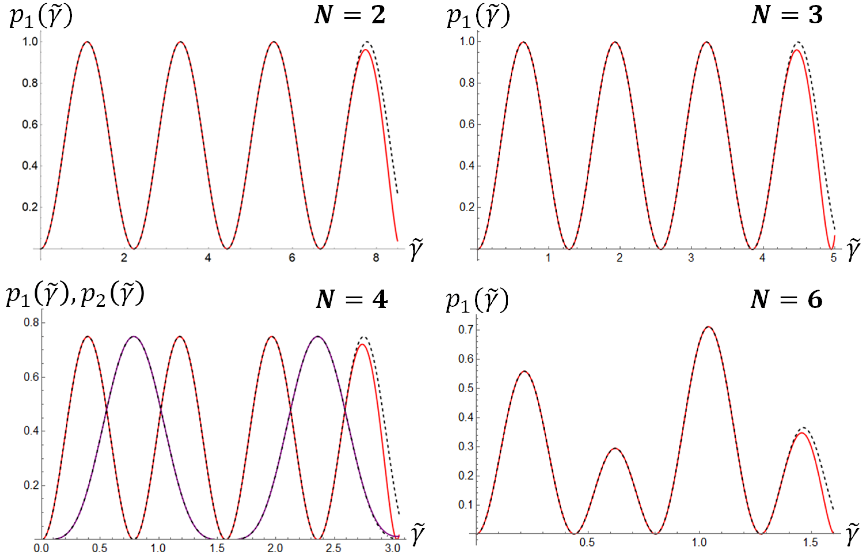
l = 1. We found out that the probability p 1 ( N , γ ˜ ) of generating a single SH photon from 2 ≤ N < 6 input photons converges, up to the order 30, to a periodic function, i.e.,
p 1 ( N , γ ˜ ) = | N 2 , 1 | ψ ( γ ˜ ) | 2 = N ! ( N 2 ) ! 1 ζ sin 2 ( ζ γ ˜ )
where:
ζ = k = 1 N / 2 k [ N 2 ( k 1 ) ] ! ( N 2 k ) ! .
The interplay among multiple creation and annihilation processes and their superposition is periodic up to six input photons, as shown in Figure 1. For N ≥ 6, this is no longer true, but still, p 1 ( N , γ ˜ ) converges to an analytic function. The reason for the aperiodic behavior of p 1 ( N , γ ˜ ) for N ≥ 6 is due to the contribution of a larger number of processes at every order, resulting in a squared sum of different periodic functions. The ratio between the periods of these functions turns out to be incommensurable, so that their sum is not a periodic function.

2.2.3. Statistics

Finally, we focus on the transformation of the statistics of the input field via SHG. We choose a particular input statistics by suitably setting the coefficients cn of the input density matrix (28). We investigate and compare the evolution of Fock, coherent, multithermal, and squeezed states. Moreover, we point out the role of the creation and annihilation processes together with their superpositions, outlined in Equation (38) by comparing the autocorrelation function for SHG (blue solid lines in the plots) with the autocorrelation function for the process k = 1 K γ ˜ 2 k N ! k ! ( N 2 k ) ! k (red dashed lines in the plots), only corresponding to the SH creation events. The latter is simply obtained by neglecting the αk and βk terms in Equation (37). Since the conversion efficiency is proportional to the input photon-number (see Equation (36)), we expect the annihilation processes and the superpositions to reduce the quantum correlations in the output state.
The moments of the output statistics are straightforward from:
n ^ SH k = Tr [ ρ ^ ( γ ˜ ) 𝟙 F n ^ k ] .
In analogy with Equation (33), the variance can be expressed as an expansion over the autocorrelation functions (32) of the input field, which here we rename g F ( 2 ) :
Δ n ^ SH 2 = g F ( 2 ) N 2 γ ˜ 2 8 3 ( g F ( 2 ) N 2 + 2 g F ( 3 ) N 3 ) γ ˜ 4 + o ( γ ˜ 6 ) = n ^ 4 3 ( g F ( 2 ) N 2 + 2 g F ( 3 ) N 3 ) γ ˜ 4 + o ( γ ˜ 6 ) .
It is possible to show that the autocorrelation function defined in Equation (32) can be written as a function of the variance and of the mean value of the number operator, so that we can compute the autocorrelation function of the SH field through:
g SH ( 2 ) = 1 + Δ n ^ SH 2 n ^ SH n ^ SH 2 .

2.2.4. Fock State

From Equation (41), we immediately get:
g SH ( 2 ) = ( N 2 ) ( N 3 ) N ( N 1 ) ( 1 + 4 γ ˜ 2 ) + o ( γ ˜ 4 ) .
which is consistent with the theoretical expectations since it is a fact (see Appendix C) that, up to the first order,
g SH ( 2 ) = g F ( 4 ) ( g SH ( 2 ) ) 2 .
The second- and fourth-order autocorrelation functions for a Fock state respectively read:
g F ( 2 ) = 1 1 N g F ( 4 ) = 1 N 3 ( N 1 ) ! ( N 4 ) !
so that, applying Equation (43), the first-order expansion for the expected second-harmonic autocorrelation function must be:
g SH ( 2 ) = ( N 2 ) ( N 3 ) N ( N 1 ) .

2.2.5. Coherent State

The case of a coherent input state can be approached by studying the evolution of Equation (28) upon requiring:
c n = e | α | 2 / 2 α n n !
where |α| is the amplitude of the generic coherent state | α = e | α | 2 k = 0 | α | 2 k / k ! | k .
Up to k = 2, the autocorrelation function reads:
g SH ( 2 ) = 1 4 3 γ ˜ 2 + o ( γ ˜ 4 )
and shows that the second-harmonic output state displays a sub-Poissonian statistics at the first perturbative order. Thus, the SH field from a coherent pump field is endowed with quantum correlations, which is due to the anti-bunching resulting from an up-conversion with efficiency proportional to Nj (Equation (36)). It is a well-known result [8,9], which has been also experimentally tested [18,19].
We here point out that, as expected, the annihilation processes and the interference between different processes contribute to reducing quantum correlations and, consequently, the nonclassicality of the output state, as shown in Figure 2.

2.2.6. Multithermal State

The probability distribution of a multithermal state reads [16]:
p μ ( n ) = n + μ 1 n 1 ( M + 1 ) μ 1 / M + 1 n ,
which is the discrete case of P(IF) (see Equation (16)). The mean number M = exp β ω 1 1 is the average boson number from the Bose–Einstein statistics [20]. If μ = 1, the well-known thermal distribution:
p ( n ) = M n ( M + 1 ) n + 1
is retrieved. The computation of the mean value and the variance from Equation (47) yields:
N = μ M
Δ N 2 = μ M ( M + 1 ) .
We note that the variance can be rewritten in terms of the mean value as Δ N 2 = N ( N / μ + 1 ) , so that it is clear that, for large mode numbers, the statistics tends to a Poissonian distribution, as expected (see the final remarks in Section 2.1). A generic input state with multithermal statistics is the mixed state ρ ^ 0 = n p μ ( n ) | n , 0 n , 0 | . Here, we write explicitly the mean value and the variance of the output statistics since this case is amenable to a comparison with the classical one:
n ^ SH = ( μ + 1 ) μ N 2 γ ˜ 2 2 3 ( μ + 1 ) μ N 2 1 + 2 μ + 2 μ N γ ˜ 4 + o ( γ ˜ 6 )
Δ n ^ SH 2 = n ^ SH + 2 ( 2 μ + 3 ) ( μ + 1 ) μ 3 N 4 γ ˜ 4 + o ( γ ˜ 6 ) .
We remark that, at the lowest orders of γ ˜ , n ^ SH and Δ n ^ SH 2 in Equations (51) and (52) exhibit the same dependence on the number of modes μ and on the input mean value N, which was retrieved in Equations (18) and (20) for the classical case.
Thus, at the first order, we find again the moments of a superthermal distribution. Furthermore, at higher orders, we still have that annihilation processes and superpositions result in a reduction of correlations, as we show in Figure 3. The computation of the SH autocorrelation function yields:
g SH ( 2 ) = ( μ + 2 ) ( μ + 3 ) μ ( μ + 1 ) 1 4 3 1 + 4 N μ γ ˜ 2 + o ( γ ˜ 4 ) .
In particular, if we compare the second panel of Figure 3 with Figure 2, we find again that if the number of modes is large, we end up with a Poissonian statistics. We remark that the contribution of the only creation processes (dashed red line) is significant to point out the effect of the back-conversion throughout the whole process, but that it has no particular physical meaning itself.

2.2.7. Squeezed State

A pure single-mode squeezed vacuum state is expanded over the number-state basis as follows [13,16]:
| ζ = 1 μ n = 0 ν 2 μ n ( 2 n ) ! n ! | 2 n
where μ = cosh(r), ν = e sinh(r), θ and r being respectively the phase and the squeezing parameter. For the sake of simplicity, we set θ = 0. The autocorrelation function for a squeezed state is given by
g F ( 2 ) = 3 + 1 N .
We found that, for such an input state, the SH autocorrelation function reads:
g SH ( 2 ) = 3 ( 1 + 3 N ) 2 [ 3 + 5 N ( 5 + 7 N ) 4 1 + 3 N ( 1 + 5 N ( 9 + 43 N 2 + 87 N 2 + 56 N 3 ) ) γ ˜ 2 ] + o ( γ ˜ 4 ) .
Firstly, we remark that the zero order in Equation (56) is the usual first approximation of the SH autocorrelation function, which is obtained through Equation (43). It is provided by the first and second orders of the perturbative expansion of the moments, then it also contains the superposition processes β2 (Equation (37)). We note that, while for a multithermal state, this contribution does not apparently affect the output correlations (see Figure 3), Figure 4 shows that for a squeezed input state, these superposition processes help to increase correlations. This is why the zero order of the SH autocorrelation function is smaller if we omit the superposition processes (red dashed line in Figure 4).
Moreover, we find that, at increasing input photon-number, g SH ( 2 ) ( 0 ) is reduced (compare the two panels in Figure 4). The same result is found for the autocorrelation function of the squeezed state (see Equation (55)), with the difference that the asymptotic value in the SH case is larger: g SH ( 2 ) ( N ) 35 3 . The fact that this value is the same as that of the zero order of the autocorrelation computed in the absence of back-conversion processes (dashed red line in Figure 4) is not accidental. From Equation (36), we know that the conversion efficiency is asymptotically smaller for higher orders, and we have superpositions just for k ≥ 2, so that their contribution is reduced as N → ∞.
Finally, we point out that, in general, the multiple back-conversion events occurring for γ ˜ > 0 contribute to reducing correlations as usual.
The high fluctuations retrieved for this SH field are a signature of the quantum properties of both the input state and the SHG process: since the squeezed state is a superposition of pairs of photons (Equation (54)) and the process always annihilates even numbers of pump photons, then SHG enhances the correlations of the input statistics.

3. Discussion

We investigated the second-harmonic generation process starting from the usual perturbative approach, but aiming to achieve some analytic results. In particular, we focused on the statistics of the output field, and helped by the comparison with the well-known classical regime, we retrieved the autocorrelation functions of the SH field for different input states, which are, as far as we know, of experimental interest. In fact, among the nonlinear parametric processes, the SHG is widely explored also in view of its multiple applications, which range from the production of laser systems with multiple wavelengths to the matching of the operation spectral range of photodetectors [21]. Moreover, nonclassical states of light are an essential resource for quantum technologies. Thus, investigating the way in which quantum optical states can be obtained through the SHG process represents a fundamental step towards their tailoring and exploitation. For instance, only a quantum approach predicts the generation of a sub-Poissonian state starting from a coherent one, a fact that is also experimentally observable.
In addition, we tried to reach a deeper understanding of the SHG process by approaching the quantum problem with different strategies and looked for the physical meaning of the perturbative terms in the expansion of the moments. In particular, we found that, at least in some cases, the conversion probability can be written in a closed form. Albeit that these latter results are not amenable for a direct experimental test, we think that they could be useful for further analytic predictions. On the one hand, an analytic formula up to a generic order k for the terms αk and βk in Equation (37), specified in Equation (38) for the first three orders, would allow us to retrieve a general expression for the moments of the SH statistics, and on the other hand, further expansions of the output SH state will lead to computing the conversion probability in more complicated cases. These two issues are both non-trivial since they require a larger number of perturbative orders, which is a computationally hard task.

Author Contributions

The authors contributed to the work in the following ways: conceptualization, G.C., M.M.W., N.F., A.A., and M.B.; validation, M.B.; formal analysis, G.C. and M.B.; investigation, G.C., M.M.W., and N.F.; writing, original draft preparation, G.C.; writing, review and editing, G.C., A.A., and M.B.; supervision, A.A. and M.B.

Funding

This research received no external funding.

Conflicts of Interest

The authors declare no conflict of interest.

Abbreviations

The following abbreviations are used in this manuscript:
SHGSecond-harmonic generation
SHSecond-harmonic

Appendix A

Theorem A1.
Given a Hamiltonian H ^ ( a ^ F , a ^ F , a ^ SH , a ^ SH ) of the form (25) with N = a ^ F a ^ F and n ^ = a ^ SH a ^ SH and assuming the initial condition a ^ SH ( 0 ) = a ^ SH ( 0 ) = 0 , then every perturbative order of n ^ can be expressed as a linear combination of the autocorrelation functions of the fundamental mode g F ( n ) in Equation (32).
Proof. 
All the terms that are a combination of ( a ^ SH ) k or a ^ SH k , with k N , do not contribute to n ^ because of the initial condition. Thus, a term survives at the kth order in the expansion of Equation (26) just if a ^ SH and a ^ SH commute, so that they are transformed into the identity, and the operators of the fundamental mode are unchanged. Moreover, the commutation relations select terms having the same number of a ^ F and a ^ F operators. The odd derivatives of n ^ all depend on the SH operators, which means that they do not contribute to n ^ and that they are given by the commutation of a ^ F and a ^ F . Therefore, the only surviving terms at a given order j are ( a ^ F ) k a ^ F k , where the exponents k are increased by two for every even derivative, but lowered by one for every odd derivative, so that k j 2 + 1 . Hence, we can conclude that n ^ is a linear combination of ( a ^ F ) k a ^ F k = γ ˜ k g F ( k ) N k .  □

Appendix B

It is well known that the autocorrelation function of order k for a Fock state | N reads:
g ( k ) = N ! N k ( N k ) ! .
As mentioned in Section 2.2, the transformation of the number state is the starting point for the analysis of the evolution of the other light distributions under investigation, from which the search of the implications of the theorem in Appendix A for an input number state follows.
Corollary A1.
If the fundamental input mode is a Fock state | ψ ( 0 ) = | N , 0 , then:
n ^ SH N j γ ˜ 2 j N j .
Proof. 
( a ^ ) k a ^ k = N ! / ( N k ) ! N k . The highest k at the order j is j 2 + 1 , but, since the odd j terms do not contribute, we only sum over the even j orders and replace j with 2j.  □

Appendix C

Up to the first order, the autocorrelation function can be approximated to Equation (43). The result is obtained through a first-order assumption on the modes, i.e., a SH = γ a F a F . Then, from Equation (41), we find:
g SH 2 = : n ^ SH n ^ SH : : n ^ SH : 2 = a ^ SH a ^ SH a ^ SH a ^ SH a ^ SH a ^ SH 2 = a ^ F a ^ F a ^ F a ^ F a ^ F a ^ F a ^ F a ^ F a ^ F a ^ F a ^ F a ^ F 2 = = a ^ F a ^ F a ^ F a ^ F a ^ F a ^ F a ^ F a ^ F a ^ F a ^ F 4 a ^ F a ^ F 2 a ^ F a ^ F a ^ F a ^ F 2 = g F 4 ( g F 2 ) 2 .

References

  1. Franken, P.A.; Hill, A.E.; Peters, C.W.; Weinreich, G. Generation of Optical Harmonics. Phys. Rev. Lett. 1961, 7, 118–120. [Google Scholar] [CrossRef]
  2. Armstrong, J.A.; Bloembergen, N.; Ducuing, J.; Pershan, P.S. Interactions between Light Waves in a Nonlinear Dielectric. Phys. Rev. 1962, 127, 1918–1939. [Google Scholar] [CrossRef] [Green Version]
  3. Bonifacio, R.; Preparata, G. Coherent Spontaneous Emission. Phys. Rev. A 1969, 2, 336–347. [Google Scholar] [CrossRef]
  4. Orszag, M.; Carrazana, P.; Chuaqui, H. Quantum Theory of Second-harmonic Generation. Opt. Acta Int. J. Opt. 1983, 30, 259–266. [Google Scholar] [CrossRef]
  5. Crosignani, B.; Di Porto, P.; Solimeno, S. Quantum effects in second harmonic generation. J. Phys. A Gen. Phys. 1972, 5, 119–121. [Google Scholar] [CrossRef]
  6. Chmela, P. Generation of light of second harmonic frequency in a Gaussian light. Czech. J. Phys. B 1973, 23, 884–887. [Google Scholar] [CrossRef]
  7. Kozierowski, M.; Tanaś, R. Quantum Fluctuations in second-harmonic light generation. Opt. Commun. 1977, 21, 229–230. [Google Scholar] [CrossRef]
  8. Bajer, J.; Perina, J. Symbolic computation of photon statistics for higher harmonics generation. Opt. Commun. 1992, 92, 99–104. [Google Scholar] [CrossRef]
  9. Bajer, J.; Haderka, O.; Perina, J. Sub-Poissonian behaviour in the second harmonic generation. J. Opt. B Quantum Semiclass. Opt. 1999, 1, 529–533. [Google Scholar]
  10. Ekert, A.; Rzazewski, K. Second harmonic generation and statistical properties of light. Opt. Commun. 1988, 65, 225–227. [Google Scholar] [CrossRef]
  11. Allevi, A.; Bondani, M. Direct detection of super-thermal photon-number statistics in second-harmonic generation. Opt. Lett. 2015, 40, 3089–3092. [Google Scholar] [CrossRef] [PubMed]
  12. Glauber, R.J. Coherent and Incoherent States of the Radiation Field. Phys. Rev. 1963, 131, 2766–2788. [Google Scholar] [CrossRef]
  13. Boyd, R.W. Nonlinear Optics, 3rd ed.; Academic Press: Cambridge, MA, USA; Elsevier: Amsterdam, The Netherlands, 2008. [Google Scholar]
  14. Qu, Y.; Singh, S. Measurements of photon statistics in second-harmonic generation. Phys. Rev. A 1995, 51, 2530–2536. [Google Scholar] [CrossRef] [PubMed]
  15. Allevi, A.; Cassina, S.; Bondani, M. Super-thermal light for imaging applications. Quantum Meas. Quantum Metrol. 2017, 4, 26–34. [Google Scholar] [CrossRef] [Green Version]
  16. Mandel, L.; Wolf, E. Optical Coherence and Quantum Optics; Cambridge University Press: Cambridge, UK, 1995. [Google Scholar]
  17. Puri, R.R. Mathematical Methods Of Quantum Optics; Springer-Verlag: Berlin/Heidelberg, Germany, 2001. [Google Scholar]
  18. Huang, J.; Kumar, P. Observation of quantum frequency conversion. Phys. Rev. Lett. 1992, 68, 2153–2156. [Google Scholar] [CrossRef] [PubMed]
  19. Youn, S.; Choi, S.-K.; Kumar, P.; Li, R.-D. Observation of sub-Poissonian light in traveling-wave second-harmonic generation. Opt. Lett. 1996, 21, 1597–1599. [Google Scholar] [CrossRef] [PubMed]
  20. Bose, S. Planck’s Law and Light Quantum Hypothesis. Z. Physic 1924, 26, 178–181. [Google Scholar] [CrossRef]
  21. Garmire, E. Nonlinear optics in daily life. Opt. Express 2013, 21, 30532–30544. [Google Scholar] [CrossRef] [PubMed]
Figure 1. Evolution of the probability of generating one SH photon from N pump photons. Solid red line: Tr [ ρ ^ ( γ ˜ ) 1 F n ^ k ] where ρ ^ is obtained by expanding U ^ in Equation (29) up to k = 30. Dashed line: theoretical prediction from Equation (39). The purple solid line in the bottom left panel is the probability of generating two photons from four. It is of the form A sin 4 ( ω γ ˜ ) .
Applsci 09 01690 g001
Figure 2. Coherent input state. Solid blue line: SH autocorrelation function, from Equation (46). Dashed line: SH autocorrelation function in the absence of annihilation processes and superpositions.
Applsci 09 01690 g002
Figure 3. Chaotic input state. Solid blue line: SH autocorrelation function, from Equation (53). Dashed line: SH autocorrelation function in the absence of annihilation processes and superpositions.
Applsci 09 01690 g003
Figure 4. Squeezed input state. Solid blue line: SH autocorrelation function, from Equation (56). Dashed line: SH autocorrelation function in the absence of annihilation processes and superpositions.
Applsci 09 01690 g004

