Compressed Learning of Deep Neural Networks for OpenCL-Capable Embedded Systems

Abstract

Deep neural networks (DNNs) have been quite successful in solving many complex learning problems. However, DNNs tend to have a large number of learning parameters, leading to a large memory and computation requirement. In this paper, we propose a model compression framework for efficient training and inference of deep neural networks on embedded systems. Our framework provides data structures and kernels for OpenCL-based parallel forward and backward computation in a compressed form. In particular, our method learns sparse representations of parameters using ${\ell }_1$-based sparse coding while training, storing them in compressed sparse matrices. Unlike the previous works, our method does not require a pre-trained model as an input and therefore can be more versatile for different application environments. Even though the use of ${\ell }_1$-based sparse coding for model compression is not new, we show that it can be far more effective than previously reported when we use proximal point algorithms and the technique of debiasing. Our experiments show that our method can produce minimal learning models suitable for small embedded devices.

1. Introduction

Modern deep neural networks (DNNs) tend to have growing numbers of parameters, which are often unavoidable to solve complex learning problems in computer vision [1], speech recognition [2], and natural language processing problems [3]. For example, the number of parameters of convolutional neural networks (CNNs) for computer vision tasks has grown. Compared to the first CNN, Lenet-5 [4], which contains less than 1M parameters, recent networks such as AlexNet [1] (60M) and VGG16 [5] (138M) consist of a much larger number of parameters.

Some networks have been optimized for their size, for example, GoogleNet (also known as Inception v1) [6], the winning method of ImageNet Large Scale Visual Recognition Challenge (ILSVRC) in 2014, only has 6.7M parameters, a surprisingly smaller number compared to the previous winners (AlexNet [1] in 2012, ZFNet [7] in 2013). However, new versions of GoogleNet such as BN-Inception [8], Inception v2 and v3 [9], and Inception v4 [10] tend to become larger for better prediction accuracy, for example, Inception v4 contains about 80M parameters. ResNet-152 [11], the winner of ILSVRC 2015 defeating Inception v3, contains 60M parameters. Other examples include Deepfaces [12] (120M parameters) and DNNs on high-performance computing systems [13] (10B parameters).

Large numbers of learning parameters, however, make it preventive to learn and apply machine learning models on small devices, e.g., smartphones, embedded computers, and wearable devices, where memory, computation, and energy consumption can be restricted. In addition, a large number of parameters may lead to overfitting, a phenomenon in machine learning that a complex and large machine learning model fits training data too much and its generalization performance on future data decreases as a result [14]. Therefore, compressing large machine learning models is an essential consideration for the training and the deployment of them in application environments such as edge computing [15] with small computation devices.

1.1. Related Work

The main idea of model compression is to reduce the effective number of parameters to be stored and computed. One of the classical ideas for DNN model compression is to use a low-rank approximation of weight matrices. This technique has been applied successfully in scene text character recognition [16], and later improved and extended for larger DNNs [17,18,19], reducing memory consumption and computational cost. However, these approaches work on fixed network architecture, requiring reiterations of decomposition, training, fine-tuning, and cross-validation.

1.1.1. Network Pruning

For the model compression of DNNs, network pruning is probably the most popular approach, which tries to remove irrelevant neural connections associated with weight values below a certain threshold. In biased weight decay [20], hyperbolic and exponential biases were introduced to the pruning objective, where brain damage [21] and brain surgeon [22] used information from the Hessian of the loss function.

More recently, Han et al. [23] suggested a network pruning approach with retraining, which performs weight training, network pruning, and then another round of weight training (retraining). The final retraining is done only for the connections not removed during the pruning step, in order to eliminate statistical bias caused by network pruning. The authors reported that pruning with ${\ell }_2$ regularization and retraining was the most successful regarding prediction accuracy, compared to ${\ell }_1$ and ${\ell }_2$ regularization alternatives with and without retraining. This method has further developed into deep compression [24], which adds two extra steps after pruning: weight quantization and the Huffman encoding. This method has been followed-up with more emphasis on compressing weights in convolutional layers, using structured sparsity regularization to induce structured sparsity in rows, columns, channels, and filters [25,26].

1.1.2. Network Pruning as Optimization

Since network pruning can be achieved by adding a regularization term in the training objective function, model compression by network pruning can be considered in terms of optimization problems. For example, stochastic optimization algorithms for ${\ell }_1$ regularization problems [27,28] have been applied to CNN model compression [29]. The forward-backward splitting algorithms in these works are closely related to our proximal point algorithms [30] to be discussed later, but only classical stochastic gradient descent has been considered in the previous work, whereas we consider more advanced training algorithms for neural networks such as RMSProp [31] and ADAM [32].

The state-of-the-art network pruning approach [33] considers reforming the network pruning into constrained optimization problems, solving them using the augmented Lagrangian method, also known as the method of multipliers [34,35]. Our proposed method also considers the penalized optimization problem as in this approach, with an important distinction that we use proximal point algorithms [30] which comes with clear benefits: lower memory consumption and faster convergence, as we show later.

Other works in model compression include guiding compression with side information such as network latency provided in forms of optimization constraints [36], designing network architecture using reinforcement learning (e.g., NAS [37] and NASNet [38]), and tuning parameters that trade-off model size and prediction accuracy automatically [39]. We refer to Cheng et al. [40] for a more detailed survey of DNN model compression.

1.2. Contribution

Even though there are quite a few works on model compression for deep neural networks, we found that they may not be well suited for learning and inference with DNNs in small embedded systems:

• Full model training is required prior to model compression: in network pruning [23,24], including the state-of-the-art method [33], and low-rank approximation [16,17,18,19], full models have to be trained first, which would be too burdensome to run on small computing devices. In addition, compression must be followed by retraining or fine-tuning steps with a substantial number of training iterations, since, otherwise, the compressed models tend to show impractically low prediction accuracy, as we show in our experiments.
• Platforms are restricted: existing approaches [23,24,25] have been implemented and evaluated mainly on CPUs because sparse weight matrices produced by model compression typically have irregular nonzero patterns and therefore are not suitable for GPU computation. In Wen et al. [25], some evaluations have been performed on GPUs, but it was implemented with a proprietary sparse matrix library (cuSPARSE) only available on the NVIDIA platforms (Santa Clara, CA, USA). He et al. [39] considered auto-tuning of model compression experimented on NVIDIA GPU and a mobile CPU on Google Pixel-1 (Mountain View, CA, USA), yet without discussion on how to implement them efficiently on embedded GPUs.

In this paper, we provide a model compression method for deep neural networks based on ${\ell }_1$-regularized optimization, often referred to as sparse coding [41,42]. Application of ${\ell }_1$-based regularization for DNNs is not entirely new; however, we discuss that it can be far more effective than previously reported. In particular, we apply ${\ell }_1$-based sparse coding with (i) proximal operators, which induce explicit sparsity in learning weights during training. In addition, it is followed by a (ii) debiasing step, which tries to reduce estimation bias due to sparse coding: we discuss that this technique allows us to compress DNNs further without sacrificing prediction accuracy much. While inducing sparsity on learning weights, we also store sparse weights in (iii) compressed data structures, being able to compute forward and backward passes with compressed weights on any (iv) OpenCL-capable devices, e.g., mobile GPUs such as ARM Mali-T880 (Cambridge, UK).

2. Method

In this section, we describe the details of our method in which network pruning is considered as an ${\ell }_1$-regularized optimization problem, i.e., sparse coding, where we aim to find a sparse representation of observations, sometimes also looking for good basis functions for such a representation (this particular task is called dictionary learning [43]). The idea of sparse coding has been applied in various fields of research, i.e., sparse regression in statistics (e.g., [44]), compressed sensing in signal processing (e.g., [45,46,47]), matrix completion in machine learning (e.g., [48]), just to name a few.

In our approach, we apply sparse coding for model compression, to find a sparse optimal weight parameters containing as many zero values as possible whenever the associated neural connections in a deep neural network are irrelevant for making an accurate prediction.

2.1. Sparse Coding in Training

To describe our method formally, let us suppose that we train a deep neural network with n examples, ${\left\{(x_i,y_i)\right\}}_{i=1}^n$, where $x_i\in {\mathbb{R}}^d$ is an input vector and $y_i\in \mathbb{R}$ (regression) or $y_i\in \{1,2,\dots ,K\}$ (classification) is the corresponding outcome. In training, we obtain the optimal weight $w^{*}\in {\mathbb{R}}^p$ by solving the following optimization problem:

$$w^{*}\in \underset{w\in {\mathbb{R}}^p}{arg\; min}\frac{1}{n}\sum _{i=1}^n\ell (w;x_i,y_i).$$

Here, $\ell (w;x_i,y_i)$ is the loss function describing the gap between the prediction made by the neural net and the desired outcome. In sparse coding, we add a regularizer $\mathsf{\Psi }\left(w\right)$ to the objective function and solve a modified training problem:

$$w^{*}\in \underset{w\in {\mathbb{R}}^p}{arg\; min}\frac{1}{n}\sum _{i=1}^n\ell (w;x_i,y_i)+\mathsf{\Psi }\left(w\right).$$

(1)

We use the ${\ell }_1$-norm $\mathsf{\Psi }\left(w\right)={\lambda \parallel w\parallel }_1$ for our method in particular, where $\lambda >0$ is a hyperparameter that controls the rate of model compression (the larger $\lambda$ is, the resulting model will be more compressed as more weight values will set to the zero value).

Note that the use of ${\ell }_1$-regularizer by itself does not automatically lead to sparse coding. We need an explicit mechanism that sets weight values to the zero value while solving Equation (1). The mechanism is called a proximal operator.

2.2. Proximal Operators

When we solve the training problem (1) for a deep neural network with a large dataset, the most popular optimization algorithms include stochastic subgradient descent [49] and its variants such as AdaGrad [50], RMSProp [31], and ADAM [32]. These methods use small subsamples of training examples $B\subset \{1,\dots ,n\}$, called minibatches, to construct stochastic subgradients in forms of:

$$g\left(w\right):=g_B\left(w\right)+\nabla \mathsf{\Psi }\left(w\right),$$

where $g_B\left(w\right):=\frac{1}{\left|B\right|}{\sum }_{i\in B}\nabla \ell (w;x_i,y_i)$ and $\nabla \mathsf{\Psi }\left(w\right)$ is a subgradient of $\mathsf{\Psi }\left(w\right)$. If we use the subgradient $g\left(w\right)$ which includes the part $\nabla \mathsf{\Psi }\left(w\right)$ from the regularizer for updating learning parameters w, it is unlikely that any updated weight value will be precisely the zero value, even though some values might be close to zero.

Instead, we consider a mechanism to set the weight values to the exact zero value whenever necessary, by means of the so-called proximal operator of a convex function $\mathsf{\Psi }(·)$. Given a vector $z\in {\mathbb{R}}^p$, the proximal operator of z with respect to $\mathsf{\Psi }$ is defined as

$${\mathrm{prox}}_{\mathsf{\Psi }}\left(z\right):=\underset{w\in {\mathbb{R}}^p}{arg\; min}\frac{1}{2}{\parallel w-z\parallel }_2^2+\mathsf{\Psi }\left(w\right).$$

When $\mathsf{\Psi }\left(w\right)={\lambda \parallel w\parallel }_1$, the regularizer we use for sparse coding, the proximal operator can be computed in a closed form independently for each component,

$${\left[{\mathrm{prox}}_{\mathsf{\Psi }}\left(z\right)\right]}_i=\mathrm{sgn}\left(z_i\right)max\left\{\right|z_i|-\lambda ,0\},i=1,\dots ,p.$$

This operator is also known as the soft-thresholding operator [51].

2.3. Optimization Algorithm

When the number of training examples n is not too large, say $n\sim 10k$, we can solve the training problem with sparse coding (1) using proximal gradient descent [30,52], which updates the weight vector at the kth iteration by:

$$w^{k+1}\leftarrow {\mathrm{prox}}_{\eta \mathsf{\Psi }}\left(w^k-\eta G\left(w^k\right)\right).$$

Here, $\eta >0$ is the learning rate and $G\left(w^k\right)$ is the full gradient involving all training examples,

$$G\left(w^k\right):=\frac{1}{n}\sum _{i=1}^n\nabla \ell (w^k;x_i,y_i).$$

The proximal gradient descent algorithm is capable of solving the regularized training problem (1) with $\mathsf{\Psi }\left(w\right)={\lambda \parallel w\parallel }_1$, while optimally fixing irrelevant weights in $w\in {\mathbb{R}}^p$ to the exact zero value. However, it will be too costly to use the method for large n, since it will require n back-propagation steps to compute the $\nabla \ell (w^k;x_i,y_i)$ for all training examples in each update.

We suggest to use a minibatch gradient $g_B\left(w\right)$ in the proximal operator so that the update will be:

$$w^{k+1}\leftarrow {\mathrm{prox}}_{\eta \mathsf{\Psi }}\left(w^k-\eta g_B\left(w^k\right)\right).$$

(2)

Due to the stochasticity in minibatch gradients, the behavior of the proximal gradient algorithm based on the update (2) will become less predictable, but some convergence results are available for the algorithm [53,54,55] (under the assumption that the loss function ℓ is convex and Lipschitz continuous in w, the objective function value converges to the optimal value with the rate $\mathcal{O}\left(k^{-1/2}\right)$ in expectation).

We further consider the update (2) within the RMSProp [31] and ADAM [32] algorithms, arguably the two most popular methods for training deep neural networks. RMSProp uses adaptive learning rates computed differently on gradient components, while ADAM combines the idea of adaptive learning rates and that of the momentum method [56] to improve convergence and to escape saddle points. We integrate proximal operators with RMSProp and ADAM: the resulting algorithms are called Prox-RMSProp (Algorithm 1) and Prox-ADAM (Algorithm 2). We can conjecture that the search directions produced by Prox-ADAM will be more stable than those of Prox-RMSProp since the former uses compositions of minibatch gradients and momentum directions, not just noisy minibatch gradients as in the latter. We show in experiments that the behavior of Prox-ADAM is indeed more stable than that of Prox-RMSProp.   

Algorithm 1. Prox-RMSProp Algorithm

Input: a learning rate $\eta$, a safeguard parameter $ϵ>0$, $\beta \in [0,1)$: a decay rate Initialize the weight vector $w\in {\mathbb{R}}^p$; $v\leftarrow 0$ (Init. 1st moment vector); $t\leftarrow 0$ (Init. timestep); while $w_t$ not converged do return $w_t$;

Algorithm 2. Prox-ADAM Algorithm

Input: a learning rate $\eta$, a safeguard parameter $ϵ>0$, ${\beta }_1,{\beta }_2\in [0,1)$: decay rates Initialize the weight vector $w\in {\mathbb{R}}^p$; $m_0\leftarrow 0$ (Init. 1st moment vector); $v_0\leftarrow 0$ (Init. 2nd moment vector); $t\leftarrow 0$ (Init. timestep); while $w_t$ not converged do

2.4. Retraining

Once we have obtained a sparse model via sparse coding, we can consider an optional step to train the weights again without any regularization, starting from the previously trained weight values, while excluding the zero-valued weights from training. This type of retraining is known as debiasing [57], which can be used to remove the unwanted reduction of weight values due to regularization. It has been shown that debiasing can improve the quality of estimation [58], although it may undo some desired effect of regularization, e.g., the reduction of distortion caused by noise [59]. Our methods work well without retraining, but our experiments show that retraining can achieve further compression without sacrificing prediction accuracy.

3. Accelerated OpenCL Operations

In order to perform forward and backward computations of deep neural networks in an accelerated manner, we must use an efficient representation of sparse weight matrices, which can be also stored in a compact form to reduce memory footprint. In the previous research, sparse data structure and matrix operations have not been discussed fully enough [23,24,25], due to the difficulty of using sparse matrix operations efficiently on GPUs. Therefore, implementations and testing were performed mainly on CPUs [23,24], or some vendor-specific support was used, e.g., the cuSPARSE library, which is not an open-source software and available only for NVIDIA hardware [25].

In this section, we discuss the details how we implement sparse weight matrices and efficient sparse matrix operations for training deep neural networks with sparse coding, making use of our proposed algorithms. We base our discussion on the OpenCL-Caffe [60] software, an OpenCL-capable version of the favorite open source deep learning software Caffe [61]. We used OpenCL-Caffe with an open source OpenCL back-end library called ViennaCL [62], which provides efficient implementations of basic linear algebra operations and some of the sparse matrix functionality.

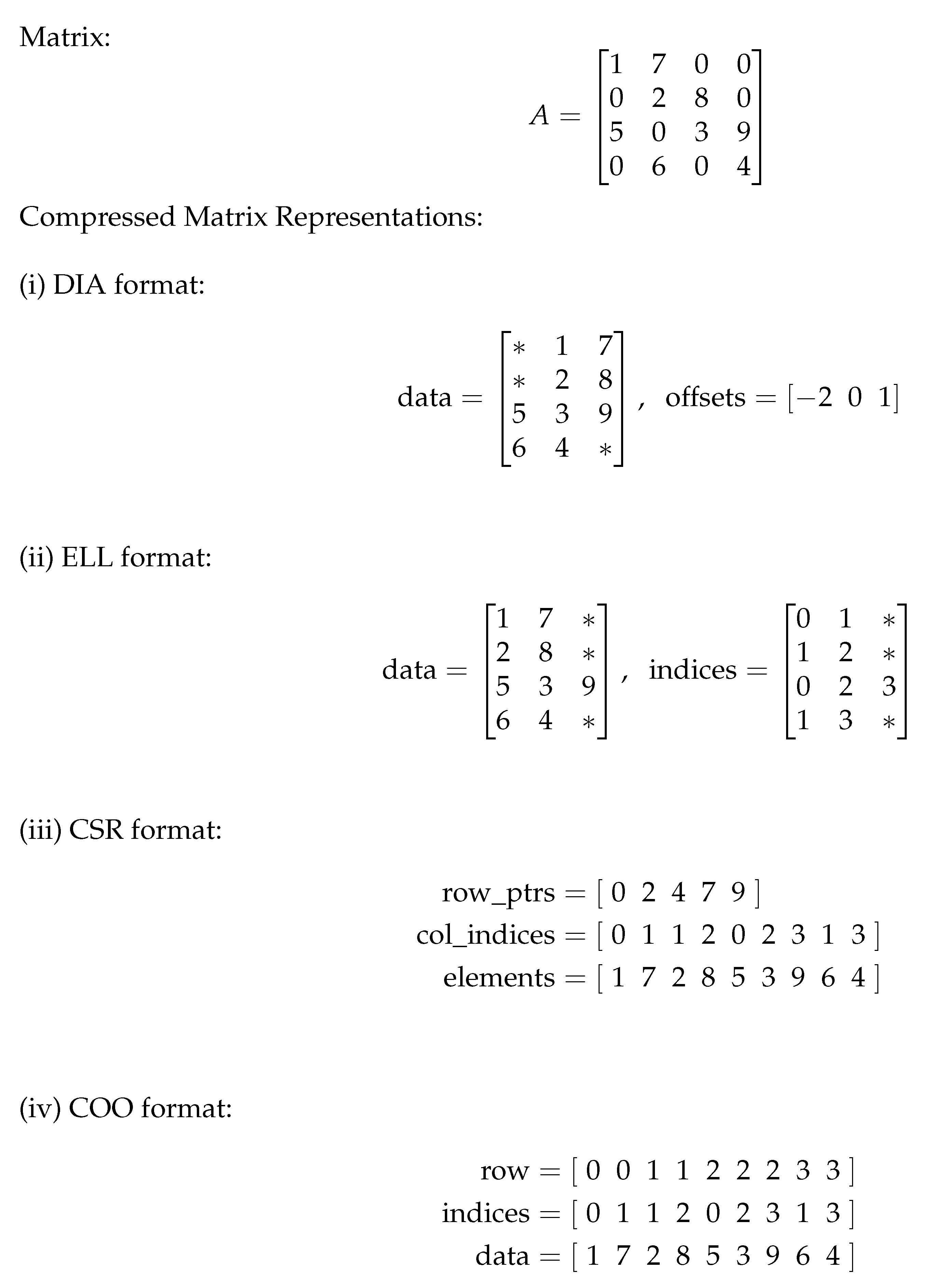
3.1. Compressed Sparse Matrix

In Section 2, we discussed how we could apply sparse coding to fix the values of irrelevant learning weights of DNNs at zero. However, if the zero values are explicitly stored in memory, the model will use the same amount of memory as the original model without compression. That is, for model compression, we need a special data structure to store only the nonzero weight values in GPU memory.

For our implementation, we have considered several popular formats, in particular, DIA, ELL, CSR, and COO matrix formats to store the sparse weight matrices [63] (see Figure 1 for comparisons of the formats). Among these, DIA is suitable for the case when nonzero values are at a small number of diagonals, and ELL is for the case when matrix rows have similar numbers of nonzero entries. Since there is usually no particular pattern of zero entries in weight matrices produced by sparse coding, we have concluded that these formats are unsuitable.

The compressed sparse row (CSR) format is probably the most popular format for representing unstructured sparse matrices. This format stores column indices and nonzero values in indices and data, respectively, while in ptr it stores the indices where new rows begin. Compared to DIA and ELL, the CSR format can store variable numbers of nonzeros in rows efficiently. The coordinate (COO) format is similar to CSR, but operations on COO can be made simpler as it also stores row indices in row for every nonzero entry. The extra storage required by COO for the row indices appears to be less economical than CSR, as our target platforms include small embedded systems. Therefore, we conclude that the CSR format will be the best for representing compressed sparse weight matrices in small, GPU-enabled devices. In ViennaCL, the CSR format is implemented as the C++ class compressed_matrix, and we have adapted this class to implement our new matrix operations for forward/backward passes of deep neural networks.

3.2. Sparse Matrix Multiplication in OpenCL

For training a deep neural network, we need efficient sparse matrix operations to deal with the compressed sparse weight matrices in the CSR format. To simplify notations, let us use W to denote the sparse weight matrix that coordinates the transfer between two consecutive DNN layers, we call the bottom and the top layers (bottom → top is the forward pass direction). Denoting by $X_B$ and $X_T$ the input from the bottom layer and the output to the top layer respectively and following the shapes and orders of matrices according to the original implementation of Caffe, we can summarize the matrix multiplications needed for the forward and the backward propagation steps as follows:

$$\begin{array}{cc}\hfill \mathrm{Forward}& :X_T\leftarrow X_B{W}^{\prime }(\mathrm{dense}\times \mathrm{compressed}{}^{\prime }),\hfill \\ \hfill \mathrm{Backward}& :\frac{\partial Loss}{\partial X_B}\leftarrow \frac{\partial Loss}{\partial X_T}W(\mathrm{dense}\times \mathrm{compressed}).\hfill \end{array}$$

Here, $X_B$ and $\frac{\partial Loss}{\partial X_T}$ are typically dense matrices, and therefore we essentially need two types of operations: dense×compressed${}^{\prime }$ ($D\times C^{\prime }$ in short), where ${}^{\prime }$ is the matrix transpose operation, and dense×compressed ($D\times C$ in short). Unfortunately, these operations are not available in the current version of ViennaCL (accessed on 19 October 2018): there exist $C\times D$ and $C\times D^{\prime }$ operations in ViennaCL, so we could use a workaround ${(C\times D^{\prime })}^{\prime }=D\times C^{\prime }$, but this requires extra memory space for transposing the result of $C\times D^{\prime }$. Furthermore, such a workaround is not available for $D\times C$ since ${(D\times C)}^{\prime }=C^{\prime }\times D^{\prime }$, and the transpose operation for compressed sparse matrices ($C^{\prime }$) is not available in ViennaCL. As a solution, we provide two new dense-compressed matrix multiplications accelerated by OpenCL.

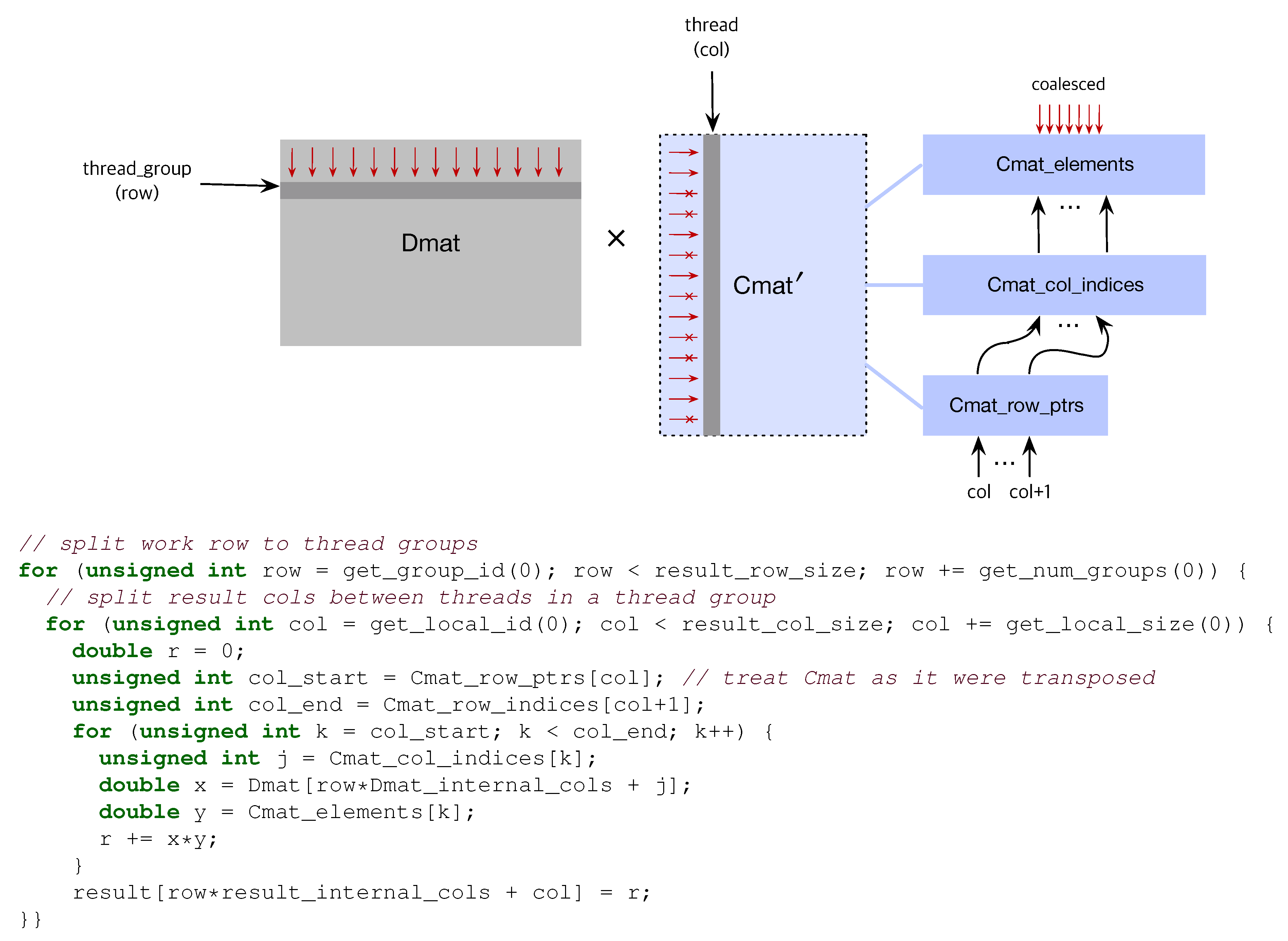
3.2.1. Dense × Compressed${}^{\prime }$

In our implementation, this operation is used for computing forward propagation. This operation is well suited for GPU acceleration, since the compressed matrix stores nonzero elements rowwise, where we access the nonzero elements stored in the compressed matrix in a rowwise fashion to compute the inner product between a row of the dense matrix and a column of the compressed${}^{\prime }$ matrix. Figure 2 shows a sketch of the operation and our OpenCL kernel code to perform this multiplication on GPUs: an OpenCL thread group is assigned to each row of Dmat (dense matrix), and multiple threads in the group will handle the assigned columns, one thread per column. For each (row, col) pair, an inner product between the row in Dmat and the column in Cmat${}^{\prime }$ (compressed${}^{\prime })$ will be computed. In our discussion hereafter, we assume that Dmat and result matrices are stored in a rowwise fashion. The column memory access of Cmat${}^{\prime }$ equals to the row access of Cmat, and therefore we can use Cmat_row_ptrs to enumerate the nonzero elements corresponding to the variable col. Each thread can access only the required nonzero elements in consecutive memory locations, and therefore thread memory access will be coalesced, leading to efficient parallelism on GPUs.

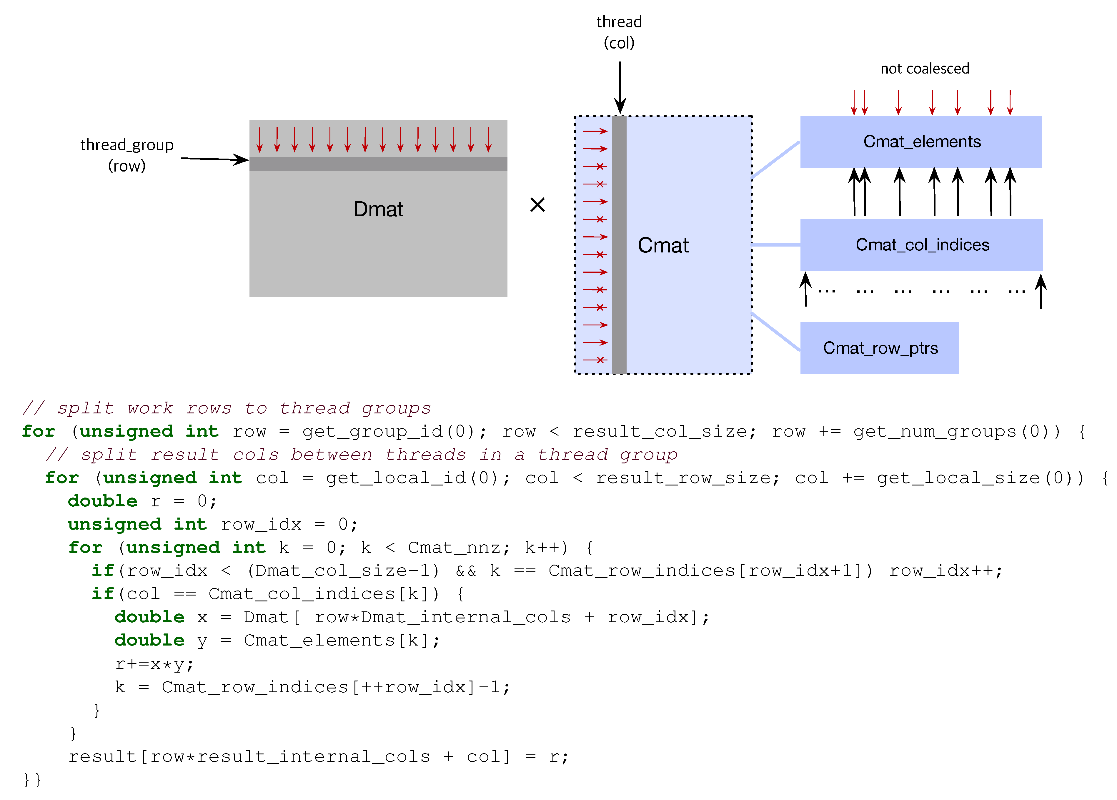
3.2.2. Dense × Compressed

This dense-compressed matrix operation is required for backward propagation. Unlike the previous one, this operation is not ideally suited for GPU parallelism since the OpenCL kernel needs to access the Cmat matrix columnwise, while the nonzero entries of the compressed matrix are stored in a rowwise fashion. Unless we store an extra array for nonzero entries stored columnwise in the compressed matrix data structure, it is unavoidable that the memory access pattern will not coalesce. Still, we can design an OpenCL kernel to parallelize the computation for each (row, col) pair, as shown in Figure 3.

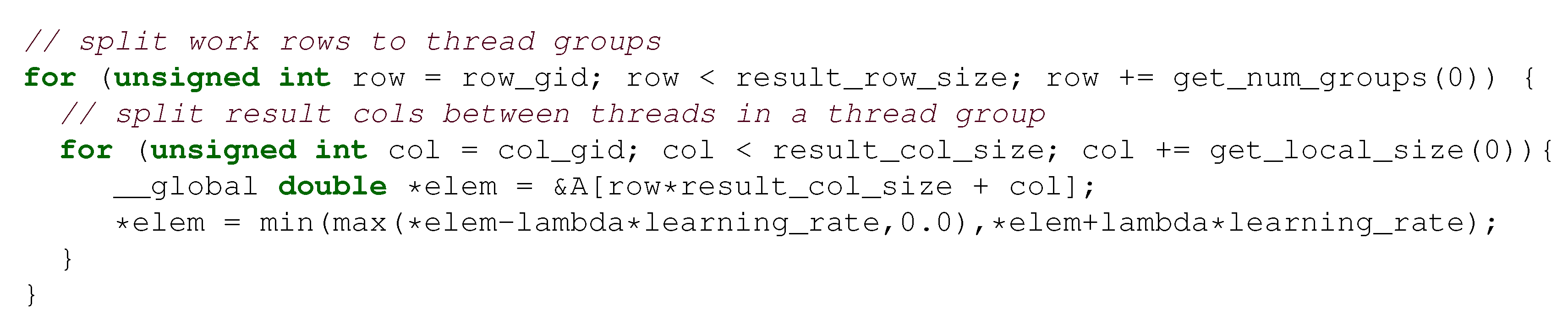
3.3. Prox Operator in OpenCL

The proximal operator discussed in Section 2.2 can be performed in parallel since the outcome can be computed elementwise, as shown in Equation (2). ViennaCL has a collection of kernels for matrix unary elementwise operations, which provides a basis for implementing our own kernel. Our code in Figure 4 assigns thread groups to rows and threads in groups to columns, similar to the two OpenCL kernels we discussed above.

4. Experiments

To show the effectiveness of our compression method for deep neural networks, we tested our method on four popular convolutional neural networks on image recognition tasks: (i) Lenet-5 on the MNIST dataset [4] and (ii) AlexNet [1], (iii) VGG16 [5], and (iv) ResNet-32 [11] on the CIFAR-10 dataset [65]. In both datasets, we have used the original split of training and test data (MNIST has $28\times 28$ grey-scaled images with no. of train/test examples = $60k/10k$, and CIFAR-10 has $32\times 32$ color images with train/test = $50k/10k$). We fixed the number of training updates to $60k$ with a minibatch size of 128 (so that the effective number of example iterations will be $60k\times 128$) since the number was large enough for the resulting neural networks to reached known top prediction accuracy. We compared our proposed method based on ${\ell }_1$-regularized sparse coding (denoted by SpC), to the existing pruning method [23] (denoted by Pru) based on thresholding and retraining and the state-of-the-art method [33] (denoted by MM) based on the method of multipliers optimization algorithm. To initialize weight values, we have used the initialization from He et al. [66], which is known to work well with neural networks containing the ReLU activation.

Our implementation is available as open-source software (https://github.com/sanglee/caffe-mc-opencl).

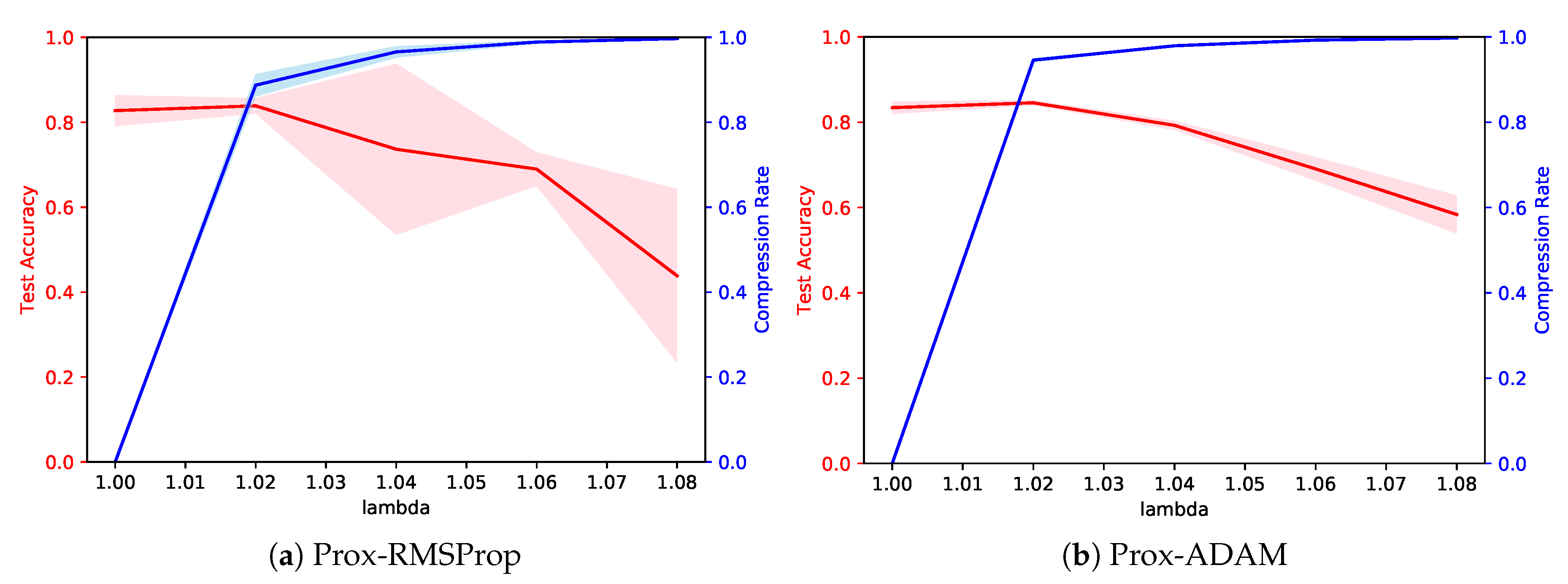
4.1. Comparison of Training Algorithms

Our algorithms Prox-RMSProp (Algorithm 1) and Prox-ADAM (Algorithm 2) use random initialization and random minibatch examples in weight updates. Furthermore, model compression will impose statistical bias compared to the reference models without compression. Hence, it is natural to expect some variation if we repeat training with different random seeds.

Here, we compare our two algorithms in order to investigate how much variation they will exhibit in training, regarding test accuracy and compression rate (the ratio of the number of zero entries to the total number of learning parameters). We have trained Lenet-5 (MNIST), AlexNet (CIFAR-10), VGGNet (CIFAR-10), ResNet-32 (CIFAR-10) multiple times with different random seeds. Amongst the experiments, our algorithms showed the most distinctive characteristics on VGGNet, as shown in Figure 5. Overall, Prox-ADAM showed smaller variance in both test accuracy and compression rate than Prox-RMSProp. This behavior is expected since the search directions produced by Prox-ADAM is more stable than those of Prox-RMSProp: in the former, the direction is a composition of a momentum direction (which brings stability) and a minibatch gradient direction, whereas in the latter it is solely based on a noisy minibatch gradient. For this reason, we chose Prox-ADAM for the rest of our experiments.

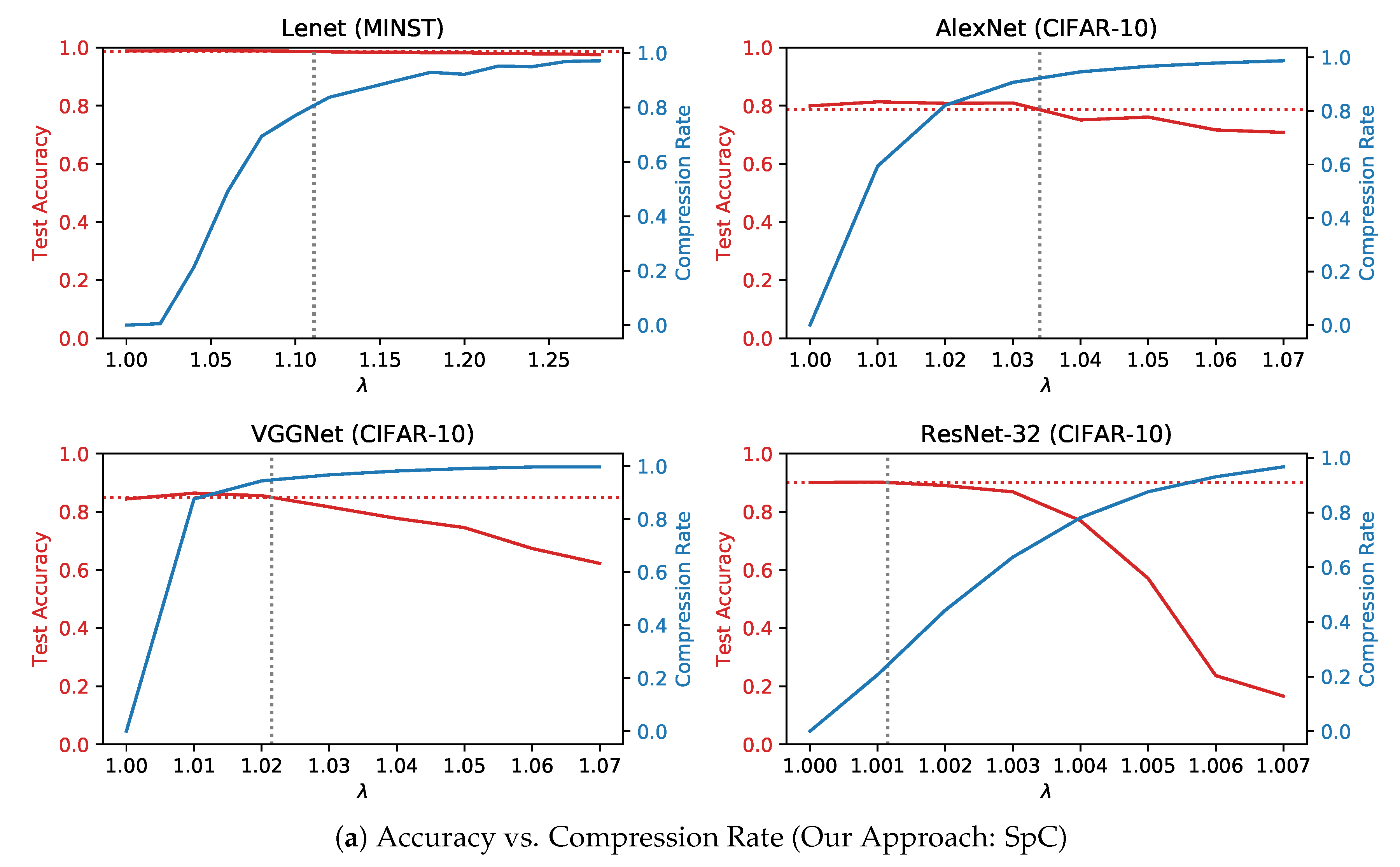
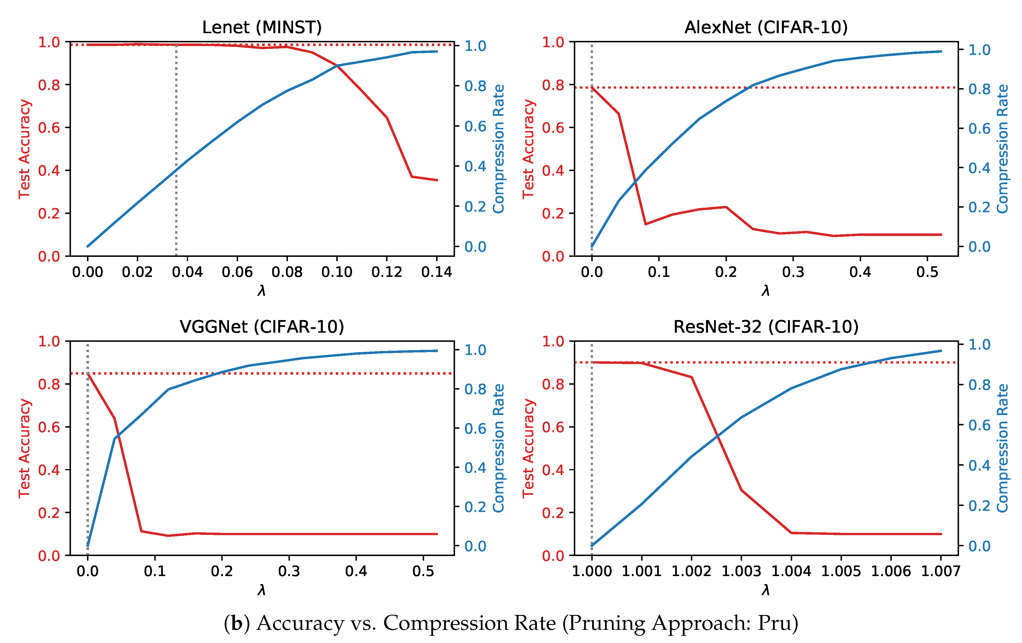
4.2. Compression Rate and Prediction Accuracy

In the training problem with sparse coding (1), we use the ${\ell }_1$-regularizer $\mathsf{\Psi }\left(w\right)={\lambda \parallel w\parallel }_1$ where $\lambda >0$ is a hyperparameter that determines the amount of compression (higher $\lambda$ gives larger numbers of zero entries in w and thereby higher compression rate).

Figure 6 shows test accuracy and compression rate of the four network-dataset pairs with respect to the change of the $\lambda$ parameter value, for our sparse coding approach (Figure 6a, SpC) and the existing pruning approach (Figure 6b, Pru). The test accuracy values of the reference networks (trained without sparse coding) are shown as the horizontal dotted lines. SpC: at small $\lambda$ values, we can see that the test accuracy of compressed models is usually better than that of the reference models. This may happen when the reference model is overfitting the data and ${\ell }_1$ regularization is mitigating the effect. When the test accuracy values of the compressed models were similar to those of the reference models (crossings of vertical and horizontal dotted lines), our method was able to remove about $90\%$ of the weights (one exception was ResNet-32, for which both Pru and SpC without retraining showed poor compression). The plots also indicate that further compression will be possible if we are ready to sacrifice prediction accuracy by a small margin. Pru: test accuracy values drop much more rapidly as we increase the compression rate, compared to our sparse coding approach. Similar test accuracy to the reference model has been achieved with about $40\%$ of compression in case of Lenet-5, but no compression was possible for AlexNet, VGGNet, and ResNet-32 if we wanted to achieve similar test accuracy to the reference model.

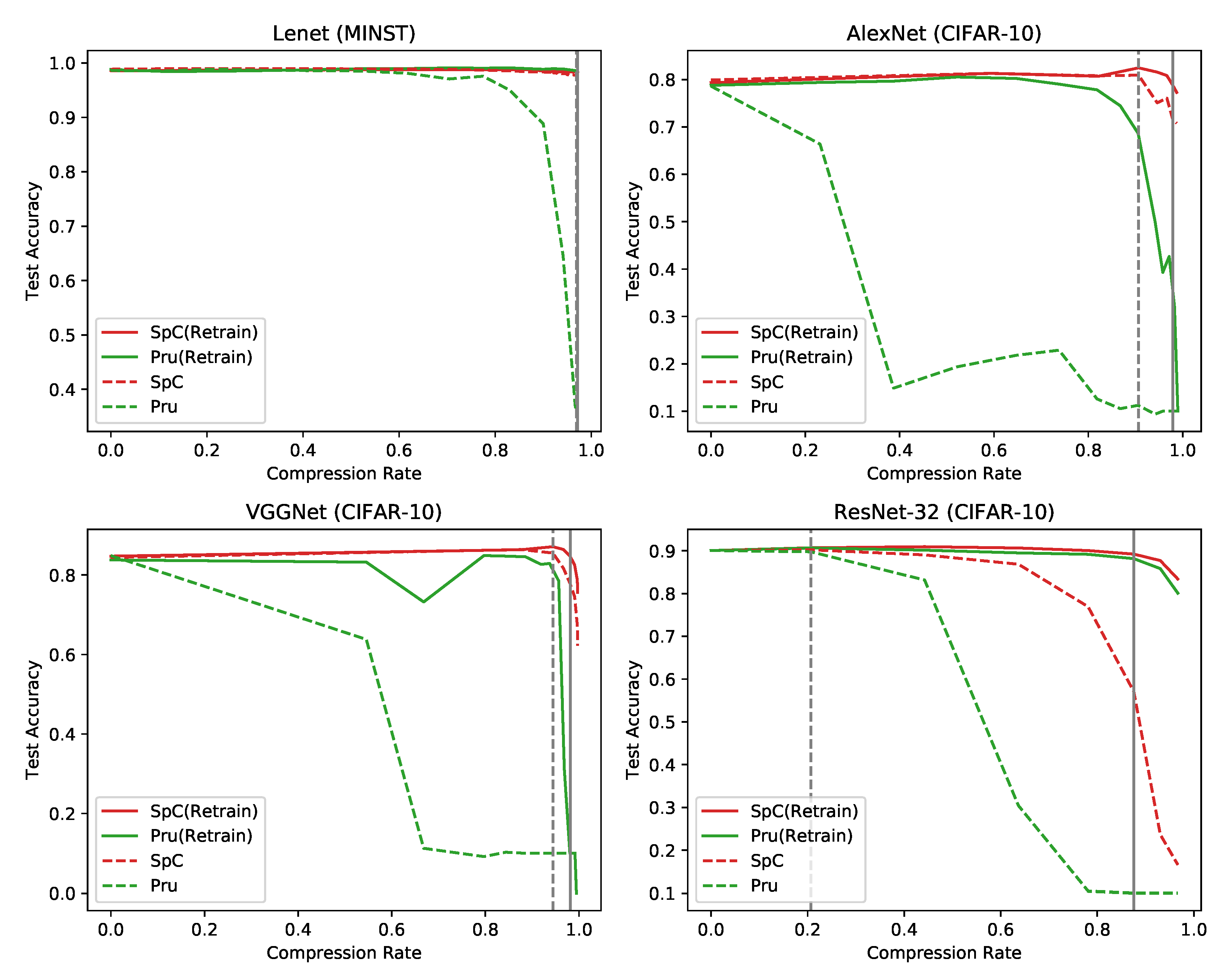
4.3. The Effect of Retraining

Compressed models can be debiased by means of an extra training the compressed networks, where the weights at the zero value are fixed and not updated during retraining. Figure 7 shows the prediction accuracy of the neural networks at different compression rates, comparing models produced by SpC and Pru, and their retrained versions, SpC(Retrain) and Pru(Retrain).

We can see that retraining is indeed a necessary step for the pruning approach (Pru) as previously known [23], since otherwise compressed models show impractically low prediction performance. The pruning method with retraining, Pru(Retrain), shows similar prediction accuracy to our sparse coding method SpC (without retraining) up to a moderate compression rate. However, when the compression rate is very high, our method SpC clearly outperforms Pru(Retrain). In addition, retraining improves the prediction accuracy of our method SpC even further, especially when the compression rate is very high, which can be seen from the solid and dotted vertical lines where SpC and SpC(Retrain), respectively, achieve at least $99\%$ of the reference accuracy with maximal compression. Therefore, for our sparse coding method SpC, retraining can be used when we aim for very high compression.

Table 1. Summary of network compression results. (Pru: network pruning, SpC: our method).

Network		Lenet-5	AlexNet	VGGNet	ResNet-32
Data		MNIST	CIFAR-10	CIFAR-10	CIFAR-10
Ref. Accuracy		$98.61\%$	$78.61\%$	$84.88\%$	$90.05\%$
Pru	Accuracy	$37.01\%$	$11.24\%$	$10.00\%$	$89.76\%$
	Compression Rate	$0.97(29\times )$	$0.91(10\times )$	$0.94(15\times )$	$0.21(1\times )$
Pru (Retrain)	Accuracy	$98.19\%$	$42.67\%$	$10.00\%$	$88.16\%$
	Compression Rate	$0.97(33\times )$	$0.97(35\times )$	$0.98(51\times )$	$0.88(8\times )$
SpC	Accuracy	$97.78\%$	$80.93\%$	$85.53\%$	$90.22\%$
	Compression Rate	$0.97(32\times )$	$0.91(10\times )$	$0.94(17\times )$	$0.21(1\times )$
SpC (Retrain)	Accuracy	$98.29\%$	$78.84\%$	$84.63\%$	$89.22\%$
	Compression Rate	$0.97(35\times )$	$0.98(47\times )$	$0.98(53\times )$	$0.88(8\times )$

summarizes the compression and prediction results of all cases.

4.4. Comparison to the State-of-the-Art Approach

We also compare our method to the state-of-the-art network pruning approach based on the method of multipliers [33], which we refer to as MM. In this method, one first duplicates the learning parameters w with an auxiliary variable $\theta$, to convert the training regularization problem (1) into the following constrained optimization problem:

$$\underset{w\in {\mathbb{R}}^p,\theta \in {\mathbb{R}}^p}{min}L\left(w\right)+\alpha \mathsf{\Psi }\left(\theta \right),\mathrm{subject}\mathrm{to}w=\theta ,$$

(3)

where $L\left(w\right)=\frac{1}{n}{\sum }_{i=1}^n\ell (w;x_i,y_i)$ is the total loss and $\mathsf{\Psi }\left(\theta \right)$ is a regularizer. Then MM constructs an augmented Lagrangian function

$$\mathcal{L}(w,\theta ,\lambda ;\mu )=L\left(w\right)+\frac{\mu }{2}{\parallel w-\theta \parallel }^2-{\lambda }^T(w-\theta )+\mathsf{\Psi }\left(\theta \right).$$

(4)

Here, $\lambda \in {\mathbb{R}}^p$ is the Lagrange multipliers and $\mu >0$ is an auxiliary parameter. Then, MM iterates (i) the minimization of $\mathcal{L}$ (in terms of w and $\theta$ in an alternating fashion) and (ii) a gradient ascent step of $\mathcal{L}$ in $\lambda$, while driving $\mu \to \infty$.

Our approach has several benefits over the MM method. First, MM requires a pre-trained model to start network pruning, whereas our method can start from random weights. Second, due to the duplication of learning weights $w\in {\mathbb{R}}^p$ by $\theta$ in Equation (3) and the introduction of the Lagrange multipliers $\lambda \in {\mathbb{R}}^p$, MM requires about double amount of memory for training than our method (ours: $(w,{\nabla }_{w}L\left(w\right))$ and MM: $(w,{\nabla }_{w}L\left(w\right),\theta ,\lambda )$). Third, the convergence of MM is quite sensitive to how we control learning rates and the auxiliary parameter $\mu \to \infty$ in the augmented Lagrangian, where our method has no such sensitivity.

Table 2. Comparison between our method SpC and the state-of-the-art MM. For MM, we used the hyperparameters and the best pretrained models as a starting point following the original paper [33]. Note that our method SpC starts from random weights and does not require complicate control of the auxiliary parameter $\mu$.

Network (Data)	Lenet-5 (MNIST)		ResNet32 (CIFAR10)
Method	SpC	MM	SpC	MM
Pretrained Model	-	Required (Test Acc = 99.1)	-	Required (Test Acc = 92.28)
Solver	Prox-Adam	SGD with Momentum	Prox-Adam	Nesterov
Aux. Parameter ($\mu$)	-	$9.76\times {10}^{-5}$ ($\times 1.1$ per 4k iter)	-	${10}^{-3}$ ($\times 1.1$ per 2k iter)
Accuracy	97.25%	97.65%	89.22%	92.37%
Compression Rate	0.98	0.98	0.88	0.85

shows the comparison between our method SpC and the state-of-the-art method MM, regarding two convolutional neural networks tested in the original paper [33]. Note that the comparison would be more favorable to MM because MM is allowed (i) to start from the state-of-the-art pretrained models and (ii) to use different solvers and auxiliary parameter control strategies as in the original paper [33]. Nevertheless, our method SpC shows a competent compression performance even though its compressed learning starts from random weight values.

Figure 8 shows the convergence behavior of SpC and MM. The compression is performed every update in SpC and every 4k updates in MM, and therefore the compression rate convergence may look smoother in MM (In fact, it is another tuning parameter in MM how often it performs weight compression, and we found that the algorithm is quite sensitive to different choices). However, our method SpC achieves the top compression rate and test accuracy much faster than MM. Therefore, our method suits better for embedded systems where we can afford only a few thousand training iterations due to time and energy constraints.

4.5. Performance on Embedded Systems

We also tested our suggested framework in an embedded system, which has a similar spec to the Samsung Galaxy S7 smartphone (Seoul, Korea). Our test system has six-core 64-bit ARM CPU, 4 GB main memory, ARM Mali-T860 GPU, OpenCL 1.2 support, and Ubuntu 16.04 operating system. In this case, we are interested in the inference time comparison between full reference models and compressed models, since in the latter the weights are stored in a compact form and will be computed with sparse matrix operations, and therefore some speedups can be expected.

Table 3. Inference speedups by model compression (Lenet-5, MNIST).

GPU	NVIDIA GTX 1080 TI		ARM Mali-T860
Compression	Yes	No	Yes	No
Model Size	148 KB	5.0 MB	148 KB	5.0 MB
Inference Time	8572 ms	16,977 ms	506,067 ms	606,699 ms
Speed up	2×		1.2×

shows the results on the test embedded system, also making a comparison to the results on a workstation with an NVIDIA GPU. Despite that we have achieved some speedup, it seems to fall short considering the size of compressed models. One reason is that the compressed convolution filters have irregular nonzero patterns for which full GPU acceleration is difficult. We plan to investigate this issue further in our future research.

5. Conclusions

In this paper, we proposed an efficient model compression framework for deep neural networks based on sparse coding with ${\ell }_1$ regularization, proximal algorithms, debiasing, and compressed computation of sparse weights using OpenCL. We believe that our method will be more versatile for embedded system applications than the previous methods as it does not require a pre-trained model as an input, while it can produce competent compressed models.

References

1. Krizhevsky, A.; Sutskever, I.; Hinton, G.E. ImageNet Classification with Deep Convolutional Neural Networks. In Advances in Neural Information Processing Systems 25; Curran Associates, Inc.: New York, NY, USA, 2012; pp. 1097–1105. [Google Scholar]
2. Graves, A.; Schmidhuber, J. Framewise phoneme classification with bidirectional LSTM and other neural network architectures. Neural Netw. 2005, 18, 5–6. [Google Scholar] [CrossRef] [PubMed]
3. Collobert, R.; Weston, J.; Bottou, L.; Karlen, M.; Kavukcuoglu, K.; Kuksa, P. Natural Language Processing (Almost) from Scratch. J. Mach. Learn. Res. 2011, 12, 2493–2537. [Google Scholar]
4. Lecun, Y.; Bottou, L.; Bengio, Y.; Haffner, P. Gradient-based learning applied to document recognition. Proc. IEEE 1998, 86, 2278–2324. [Google Scholar] [CrossRef] [Green Version]
5. Simonyan, K.; Zisserman, A. Very Deep Convolutional Networks for Large-Scale Image Recognition. In Proceedings of the International Conference on Learning Representations, San Diego, CA, USA, 7–9 May 2015. [Google Scholar]
6. Szegedy, C.; Liu, W.; Jia, Y.; Sermanet, P.; Reed, S.; Anguelov, D.; Erhan, D.; Vanhoucke, V.; Rabinovich, A. Going Deeper with Convolutions. In Proceedings of the Computer Vision and Pattern Recognition (CVPR), Boston, MA, USA, 7–12 June 2015. [Google Scholar]
7. Zeiler, M.D.; Fergus, R. Visualizing and Understanding Convolutional Networks. In Proceedings of the Computer Vision (ECCV 2014), Zurich, Switzerland, 6–12 September 2014; pp. 818–833. [Google Scholar]
8. Ioffe, S.; Szegedy, C. Batch Normalization: Accelerating Deep Network Training by Reducing Internal Covariate Shift. In Proceedings of the 32nd International Conference on Machine Learning, Lille, France, 6–11 July 2015; pp. 448–456. [Google Scholar]
9. Szegedy, C.; Vanhoucke, V.; Ioffe, S.; Shlens, J.; Wojna, Z. Rethinking the Inception Architecture for Computer Vision. In Proceedings of the IEEE Conference on Computer Vision and Pattern Recognition (CVPR), Las Vegas, NV, USA, 26 June–1 July 2016; pp. 2818–02826. [Google Scholar]
10. Szegedy, C.; Ioffe, S.; Vanhoucke, V.; Alemi, A.A. Inception-v4, Inception-ResNet and the Impact of Residual Connections on Learning. In Proceedings of the Thirty-First AAAI Conference on Artificial Intelligence, San Francisco, CA, USA, 4–9 February 2017; pp. 4278–4284. [Google Scholar]
11. He, K.; Zhang, X.; Ren, S.; Sun, J. Deep Residual Learning for Image Recognition. In Proceedings of the IEEE Conference on Computer Vision and Pattern Recognition, Las Vegas, NV, USA, 27–30 June 2016; pp. 770–778. [Google Scholar]
12. Taigman, Y.; Yang, M.; Ranzato, M.; Wolf, L. DeepFace: Closing the Gap to Human-Level Performance in Face Verification. In Proceedings of the IEEE Conference on Computer Vision and Pattern Recognition (CVPR), Columbus, OH, USA, 23–28 June 2014. [Google Scholar]
13. Coates, A.; Huval, B.; Wang, T.; Wu, D.; Catanzaro, B.; Andrew, N. Deep learning with COTS HPC systems. In Proceedings of the 30th International Conference on Machine Learning, Atlanta, GA, USA, 16–21 June 2013; pp. 1337–1345. [Google Scholar]
14. Lawrence, S.; Giles, C.L.; Tsoi, A.C. Lessons in Neural Network Training: Overfitting May be Harder than Expected. In Proceedings of the Fourtheenth National Conference on Artificial Intelligence (AAAI’97), Providence, RI, USA, 27–31 July 1997. [Google Scholar]
15. Buyya, R.; Yeo, C.S.; Venugopal, S.; Broberg, J.; Brandic, I. Cloud Computing and Emerging IT Platforms: Vision, Hype, and Reality for Delivering Computing As the 5th Utility. Future Gener. Comput. Syst. 2009, 25, 599–616. [Google Scholar] [CrossRef]
16. Jaderberg, M.; Vedaldi, A.; Zisserman, A. Speeding up Convolutional Neural Networks with Low Rank Expansions. In Proceedings of the British Machine Vision Conference, Nottingham, UK, 1–5 September 2014. [Google Scholar]
17. Denton, E.; Zaremba, W.; Bruna, J.; LeCun, Y.; Fergus, R. Exploiting Linear Structure Within Convolutional Networks for Efficient Evaluation. In Advances in Neural Information Processing Systems 27; Curran Associates, Inc.: New York, NY, USA, 2014; pp. 1269–1277. [Google Scholar]
18. Ioannou, Y.; Robertson, D.P.; Shotton, J.; Cipolla, R.; Criminisi, A. Training cnns with low-rank filters for efficient image classification. In Proceedings of the International Conference on Learning Representations, San Juan, PR, USA, 2–4 May 2016. [Google Scholar]
19. Tai, C.; Xiao, T.; Wang, X.; E, W. Convolutional neural networks with low-rank regularization. In Proceedings of the International Conference on Learning Representations, San Juan, PR, USA, 2–4 May 2016. [Google Scholar]
20. Hanson, S.J.; Pratt, L.Y. Comparing Biases for Minimal Network Construction with Back-Propagation. In Advances in Neural Information Processing Systems 1; Morgan-Kaufmann: Burlington, MA, USA, 1989; pp. 177–185. [Google Scholar]
21. LeCun, Y.; Denker, J.S.; Solla, S.A. Optimal Brain Damage. In Advances in Neural Information Processing Systems 2; Morgan-Kaufmann: Burlington, MA, USA, 1990; pp. 598–605. [Google Scholar]
22. Hassibi, B.; Stork, D.G. Second order derivatives for network pruning: Optimal Brain Surgeon. In Advances in Neural Information Processing Systems 5; Morgan-Kaufmann: Burlington, MA, USA, 1993; pp. 164–171. [Google Scholar]
23. Han, S.; Pool, J.; Tran, J.; Dally, W.J. Learning Both Weights and Connections for Efficient Neural Networks. In Advances in Neural Information Processing Systems 28; Curran Associates, Inc.: New York, NY, USA, 2015; pp. 1135–1143. [Google Scholar]
24. Han, S.; Mao, H.; Dally, W.J. Deep Compression: Compressing Deep Neural Networks with Pruning, Trained Quantization and Huffman Coding. In Proceedings of the International Conference on Learning Representations, San Juan, PR, USA, 2–4 May 2016. [Google Scholar]
25. Wen, W.; Wu, C.; Wang, Y.; Chen, Y.; Li, H. Learning Structured Sparsity in Deep Neural Networks. In Proceedings of the 30th International Conference on Neural Information Processing Systems (NIPS’16), Barcelona, Spain, 5–10 December 2016; pp. 2082–2090. [Google Scholar]
26. Lebedev, V.; Lempitsky, V. Fast ConvNets Using Group-Wise Brain Damage. In Proceedings of the IEEE Conference on Computer Vision and Pattern Recognition (CVPR), Las Vegas, NV, USA, 27–30 June 2016; pp. 2554–2564. [Google Scholar]
27. Shalev-Shwartz, S.; Tewari, A. Stochastic Methods for l1 Regularized Loss Minimization. In Proceedings of the 26th International Conference on Machine Learning (ICML), Montreal, QC, Canada, 14–18 June 2009; pp. 929–936. [Google Scholar]
28. Duchi, J.C.; Singer, Y. Efficient Learning using Forward-Backward Splitting. In Advances in Neural Information Processing Systems 22; Curran Associates, Inc.: New York, NY, USA, 2009; pp. 495–503. [Google Scholar]
29. Zhou, H.; Alvarez, J.M.; Porikli, F. Less Is More: Towards Compact CNNs. In Computer Vision (ECCV 2016); Springer: New York, NY, USA, 2016; pp. 662–677. [Google Scholar]
30. Parikh, N.; Boyd, S. Proximal Algorithms. Found. Trends Optim. 2014, 1, 127–239. [Google Scholar] [CrossRef] [Green Version]
31. Hinton, G. CSC321. Introduction to Neural Networks and Machine Learning; Lecture 6e.; Toronto University: Toronto, ON, Canada, February 2014. [Google Scholar]
32. Kingma, D.P.; Ba, J.L. Adam: A Method for Stochastic Optimization. In Proceedings of the International Conference on Learning Representations, San Diego, CA, USA, 7–9 May 2015. [Google Scholar]
33. Carreira-Perpiñán, M.Á.; Idelbayev, Y. Learning-Compression Algorithms for Neural Net Pruning. In Proceedings of the IEEE Conference on Computer Vision and Pattern Recognition (CVPR), Salt Lake City, UT, USA, 18–22 June 2018. [Google Scholar]
34. Hestenes, M.R. Multiplier and gradient methods. J. Optim. Theory Appl. 1969, 4, 303–320. [Google Scholar] [CrossRef]
35. Powell, M.J.D. A method for nonlinear constraints in minimization problems. In Optimization; Fletcher, R., Ed.; Academic Press: New York, NY, USA, 1969; pp. 283–298. [Google Scholar]
36. Chen, C.; Tung, F.; Vedula, N.; Mori, G. Constraint-Aware Deep Neural Network Compression. In Proceedings of the European Conference on Computer Vision (ECCV), Munich, Germany, 8–14 September 2018. [Google Scholar]
37. Zoph, B.; Le, Q.V. Neural Architecture Search with Reinforcement Learning. arXiv 2016, arXiv:1611.01578. [Google Scholar]
38. Zoph, B.; Vasudevan, V.; Shlens, J.; Le, Q.V. Learning Transferable Architectures for Scalable Image Recognition. arXiv 2017, arXiv:1707.07012. [Google Scholar]
39. He, Y.; Lin, J.; Liu, Z.; Wang, H.; Li, L.J.; Han, S. AMC: AutoML for Model Compression and Acceleration on Mobile Devices. In Proceedings of the European Conference on Computer Vision (ECCV), Munich, Germany, 8–14 September 2018. [Google Scholar]
40. Cheng, Y.; Wang, D.; Zhou, P.; Zhang, T. Model Compression and Acceleration for Deep Neural Networks: The Principles, Progress, and Challenges. IEEE Signal Process. Mag. 2018, 35, 126–136. [Google Scholar] [CrossRef]
41. Lee, H.; Battle, A.; Raina, R.; Ng, A.Y. Efficient sparse coding algorithms. In Advances in Neural Information Processing Systems 19; MIT Press: Cambridge, MA, USA, 2007; pp. 801–808. [Google Scholar]
42. Needell, D.; Tropp, J. CoSaMP: Iterative signal recovery from incomplete and inaccurate samples. Appl. Comput. Harmon. Anal. 2009, 26, 301–321. [Google Scholar] [CrossRef] [Green Version]
43. Bao, C.; Ji, H.; Quan, Y.; Shen, Z. Dictionary Learning for Sparse Coding: Algorithms and Convergence Analysis. IEEE Trans. Pattern Anal. Mach. Intell. 2016, 38, 1356–1369. [Google Scholar] [CrossRef]
44. Tibshirani, R. Regression Shrinkage and Selection via the Lasso. J. R. Stat. Soc. (Ser. B) 1996, 58, 267–288. [Google Scholar] [CrossRef]
45. Candes, E.; Tao, T. The Dantzig Selector: Statistical Estimation When P Is Much Larger Than N. Ann. Stat. 2007, 35, 2313–2351. [Google Scholar] [CrossRef]
46. Candes, E.J.; Tao, T. Decoding by linear programming. IEEE Trans. Inf. Theory 2005, 51, 4203–4215. [Google Scholar] [CrossRef] [Green Version]
47. Donoho, D.L. Compressed sensing. IEEE Trans. Inf. Theory 2006, 52, 1289–1306. [Google Scholar] [CrossRef]
48. Candes, E.; Plan, Y. Matrix Completion with Noise. Proc. IEEE 2010, 98, 925–936. [Google Scholar] [CrossRef]
49. Nemirovski, A.; Juditsky, A.; Lan, G.; Shapiro, A. Robust Stochastic Approximation Approach to Stochastic Programming. SIAM J. Optim. 2009, 19, 1574–1609. [Google Scholar] [CrossRef]
50. Duchi, J.; Hazan, E.; Singer, Y. Adaptive Subgradient Methods for Online Learning and Stochastic Optimization. J. Mach. Learn. Res. 2011, 12, 2121–2159. [Google Scholar]
51. Lee, S.; Wright, S. Manifold Identification of Dual Averaging Methods for Regularized Stochastic Online Learning. In Proceedings of the 28th International Conference on Machine Learning (ICML), Bellevue, WA, USA, 28 June–2 July 2011; pp. 1121–1128. [Google Scholar]
52. Auslender, A.; Teboulle, M. Interior Gradient and Proximal Methods for Convex and Conic Optimization. SIAM J. Optim. 2006, 16, 697–725. [Google Scholar] [CrossRef]
53. Nitanda, A. Stochastic Proximal Gradient Descent with Acceleration Techniques. In Advances in Neural Information Processing Systems 27; Curran Associates, Inc.: New York, NY, USA, 2014; pp. 1574–1582. [Google Scholar]
54. Patrascu, A.; Necoara, I. Nonasymptotic convergence of stochastic proximal point methods for constrained convex optimization. J. Mach. Learn. Res. 2018, 18, 1–42. [Google Scholar]
55. Rosasco, L.; Villa, S.; Vu, B.C. Convergence of Stochastic Proximal Gradient Algorithm. arXiv 2014, arXiv:1403.5074. [Google Scholar]
56. Polyak, B.T. Some methods of speeding up the convergence of iteration method. USSR Comput. Math. Math. Phys. 1964, 4, 1–17. [Google Scholar] [CrossRef]
57. Wright, S.J.; Nowak, R.D.; Figueiredo, M.A.T. Sparse reconstruction by separable approximation. IEEE Trans. Signal Process. 2009, 57, 2479–2493. [Google Scholar] [CrossRef]
58. Figueiredo, M.; Nowak, R.; Wright, S. Gradient projection for sparse reconstruction: application to compressed sensing and other inverse problems. IEEE J. Sel. Top. Signal Process. 2007, 1, 586–598. [Google Scholar] [CrossRef]
59. Donoho, D. De-noising by soft thresholding. IEEE Trans. Inf. Theory 1995, 41, 6–18. [Google Scholar] [CrossRef]
60. OpenCL-Caffe. Available online: https://github.com/amd/OpenCL-caffe (accessed on 31 August 2018).
61. Jia, Y.; Shelhamer, E.; Donahue, J.; Karayev, S.; Long, J.; Girshick, R.; Guadarrama, S.; Darrell, T. Caffe: Convolutional Architecture for Fast Feature Embedding. arXiv 2014, arXiv:1408.5093. [Google Scholar]
62. ViennaCL. Available online: http://viennacl.sourceforge.net (accessed on 31 August 2018).
63. Bell, N.; Garland, M. Efficient Sparse Matrix-Vector Multiplication on CUDA; NVIDIA Technical Report NVR-2008-004; NVIDIA Corporation: Santa Clara, CA, USA, 2008. [Google Scholar]
64. Bell, N.; Garland, M. Implementing Sparse Matrix-vector Multiplication on Throughput-oriented Processors. In Proceedings of the Conference on High Performance Computing Networking, Storage and Analysis, Portland, OR, USA, 14–20 November 2009; Volume 18, pp. 1–11. [Google Scholar]
65. Krizhevsky, A. Learning Multiple Layers of Features from Tiny Images; Technical Report; University of Toronto: Toronto, ON, Canada, 2009. [Google Scholar]
66. He, K.; Zhang, X.; Ren, S.; Sun, J. Delving Deep into Rectifiers: Surpassing Human-Level Performance on ImageNet Classification. In Proceedings of the 2015 IEEE International Conference on Computer Vision (ICCV ’15), Santiago, Chile, 11–18 December 2015; pp. 1026–1034. [Google Scholar]
Figure 1. Compressed matrix representation of a simple matrix A. The entries marked by ∗ are padding entries ([64], Figure 2).
Applsci 09 01669 g001
Figure 2. OpenCL kernel for the Dense(Dmat) × Compressed(Cmat) operation.
Applsci 09 01669 g002
Figure 3. OpenCL kernel for the Dense(Dmat) × Compressed(Cmat) operation.
Applsci 09 01669 g003
Figure 4. OpenCL kernel for the proximal operator, where the matrix A contains w k η G ( w k ) .
Applsci 09 01669 g004
Figure 5. Comparison of our suggested algorithms (a) Prox-RMSProp and (b) Prox-ADAM, on VGGNet training with the CIFAR-10 dataset. Prox-ADAM produced more stable trained models in terms of test accuracy and compression rate.
Applsci 09 01669 g005
Figure 6. Compression rate and test accuracy with respect to the change of the λ parameter value, for (a) our sparse coding approach Spc and (b) the existing pruning approach. Higher λ values result in more compression with a decrease in prediction accuracy. (a) Spc: using sparse coding, about 90 % of model parameters can be compressed achieving similar prediction accuracy to the reference models (test accuracy is shown as the horizontal dotted lines, and their crossings with accuracy curves of compressed models are marked as vertical dotted lines); (b) Pru: the existing pruning approach does not compress the networks as much: about 40 % compression for Lenet-5 but no compression for the other networks at the similar accuracy level to the reference model.
Applsci 09 01669 g006aApplsci 09 01669 g006b
Figure 7. The effect of retraining. The maximal compression rates where our methods SpC and SpC(Retrain) achieve at least 99 % of the reference prediction accuracy are indicated by vertical lines (solid: SpC, dotted: SpC(Retrain)). Retraining is indeed required for Pru since otherwise high compression rate is not possible to achieve good prediction performance. On the contrary, our method SpC without retraining can achieve high accuracy at high compression. Retraining for SpC can be considered when we aim for very high compression.
Applsci 09 01669 g007
Figure 8. Convergence behavior of the our method SpC (left) and the state-of-the-art MM (right) in terms of compression rate and test accuracy on Lenet-5 (MNIST). Our method SpC reaches top accuracy and compression much faster than MM. Note that the last iterations are 60k (SpC) and 120k (MM).
Applsci 09 01669 g008