Evaluation of Weighting Average Functions as a Simplification of the Radiative Transfer Simulation in Vertically Inhomogeneous Eutrophic Waters

Abstract

Current water color remote sensing algorithms typically do not consider the vertical variations of phytoplankton. Ecolight with a radiative transfer program was used to simulate the underwater light field of vertical inhomogeneous waters based on the optical properties of a eutrophic lake (i.e., Lake Chaohu, China). Results showed that the vertical distribution of chlorophyll-a (Chla(z)) can considerably affect spectrum shape and magnitude of apparent optical properties (AOPs), including subsurface remote sensing reflectance in water (r_rs(λ, z)) and the diffuse attenuation coefficient (K_x(λ, z)). The vertical variations of Chla(z) changed the spectrum shapes of r_rs(λ, z) at the green and red wavelengths with a maximum value at approximately 590 nm, and changed the K_x(λ, z) from blue to red wavelength range with no obvious spectral variation. The difference between r_rs(λ, z) at depth z m and its asymptotic value (Δr_rs(λ, z)) could reach to ~78% in highly stratified waters. Diffuse attenuation coefficient of downwelling plane irradiance (K_d(λ, z)) had larger vertical variations, especially near water surface, in highly stratified waters. Three weighting average functions performed well in less stratified waters, and the weighting average function proposed by Zaneveld et al., (2005) performed best in highly stratified waters. The total contribution of the first three layers to r_rs(λ, 0⁻) was approximately 90%, but the contribution of each layer in the water column to r_rs(λ, 0⁻) varied with wavelength, vertical distribution of Chla(z) profiles, concentration of suspended particulate inorganic matter (SPIM), and colored dissolved organic matter (CDOM). A simple stratified remote sensing reflectance model considering the vertical distribution of phytoplankton was built based on the contribution of each layer to r_rs(λ, 0⁻).

1. Introduction

The frequent occurrence of algal blooms in eutrophic lakes is a worldwide problem that threatens ecological and environmental safety, drinking water resources, and human activities. Under the regulation of self-buoyancy and environmental conditions (e.g., light intensity, wind, waves), algae can move up and down in the water column, and exhibit a vertically inhomogeneous distribution of chlorophyll-a (Chla(z), z refers to water depth,

Table 1. Acronyms, abbreviations, and symbols of the parameters used in this study.

Acronyms and Abbreviations
AOPs	Apparent optical properties
CDOM	Colored dissolved organic matter
IOPs	Inherent optical properties
OACs	Optically active constituents
Symbols
a(λ)	Total absorption coefficient at λ nm (m−1)
ag(λ)	Absorption coefficient of CDOM at λ nm (m−1)
bb(λ)	Total backscattering coefficient at λ nm (m−1)
Chla	Chlorophyll-a concentration (mg/m3)
Chla(z)	Vertical profile of chlorophyll-a concentration at water depth z m (mg/m3), described by three parameters: C0, h, and σ
Ed(λ, z)	Downwelling plane irradiance at λ nm and water depth z m (W m−2 nm−1)
Eu(λ, z)	Upwelling plane irradiance at λ nm and water depth z m (W m−2 nm−1)
Fr(z1, z2)	Fraction of rrs(λ,0−) at the layer between z1 m and z2 m
G(λ, z)	= rrs(λ, z)/(bb(λ, z)/(a(λ, z) + bb(λ, z)))
gGC	Average weighting function derived by Gordon and Clark (1980) [8]
gS	Average weighting function derived by Sokoletsky and Yacobi (2011) [9]
gx	Average weighting function, x represents the different functions
gZ	Average weighting function derived by Zaneveld et al. (2005) [10]
IOP’(λ, z)	= bb(λ, z)/(a(λ, z) + bb(λ, z))
Lu(λ, z)	Upwelling radiance at λ nm and water depth z m (W m−2 sr−1 nm−1)
Kd	Diffuse attenuation coefficient of downwelling plane irradiance (m−1)
KLu	Diffuse attenuation coefficient of upwelling radiance (m−1)
Ku	Diffuse attenuation coefficient of upwelling plane irradiance (m−1)
rrs(0−)	Remote sensing reflectance just below the water surface (sr−1)
rrs(z)	Remote sensing reflectance at water depth z m (sr−1)
rrs(zb)	The asymptotic value of rrs(z) at deep water zb m (sr−1)
Rrs(λ)	Remote sensing reflectance just above the water surface at λ nm (sr−1)
rrs-v(0−)	Model derived rrs(0−)of stratified waters (sr−1)
θ	Solar zenith angle (°)
Sg	Spectral slope of ag spectrum from 400 to 700 nm (nm−1)
SPIM	Suspended particulate inorganic matter (mg/L)

). The Gaussian and shifted Gaussian models have often been used to illustrate the vertical non-uniform profiles of phytoplankton in oceanic waters [1,2,3,4,5,6]. Meanwhile, four vertical distribution classes (vertically uniform, Gaussian, exponential, and hyperbolic) of Chla(z), with the maximum value on the water surface, were observed in a shallow eutrophic lake (i.e., Lake Chaohu, China) with a large content of cyanobacteria [7].

Ocean color remote sensing has been extensively used to monitor eutrophication by estimating the concentrations of Chla [11,12] and phycocyanin (PC) [13,14], area, and frequency of algal blooms [1,2,15,16] in oceanic, coastal, and inland waters. Notably, remote sensing reflectance (R_rs(λ)) is related to the optical characteristics of water constituents within a certain depth [17]. However, current remote sensing inversion models are typically developed based on the relationship between R_rs(λ) and bio-optical parameters near the water surface, or based on the assumption that Chla and the corresponding inherent optical properties (IOPs) are vertically uniform. In fact, the inhomogeneous distribution of phytoplankton considerably affects the spectrum shape and magnitude of R_rs(λ) [18,19,20]. The differences in R_rs(λ) between the vertical nonuniform and uniform water can be as high as >70% when the near-surface Chla decreases dramatically with depth [21]. Vertical variations of Chla(z) and IOPs(z) would introduce large errors in estimation of optical parameters using water color inversion algorithms built based on the assumption of vertical homogeneity [19,21,22].

Apparent optical properties (AOPs) are optical properties that depend on IOPs and ambient light [23]. The underwater light field depends on the sun’s position, the wavelength of light, the scattering and absorption properties of water constitutes, water depth, aerosols, roughness of water surface, and cloud conditions [23,24]. The radiative transfer equation (RTE) provides a connection between IOPs and AOPs. Several approaches, including Monte Carlo simulation [25,26,27,28], the invariant imbedding method [23], and the discrete ordinate method [29], have been used to obtain numerical solutions for the RTE of water via the necessary boundary conditions. Several vector radiative transfer models of coupled ocean–atmosphere system (e.g., studies in References [30,31,32,33,34,35,36]) were developed to predict the radiance and degree of polarization of the light using various numerical methods.

Through theoretical analyses and numerical modeling, sub-surface remote sensing reflectance (r_rs(0⁻)) was determined to be generally proportional to the ratio of b_b/(a + b_b), where a is the absorption coefficient and b_b is the backscattering coefficient [37,38]. The most extensively used forward remote sensing model was reported by Gordon et al. [39] and is expressed as follows:

$$r_{rs}(0^{-})=g\frac{b_b}{a+b_b},$$

(1)

$$g=g_0+g_1\frac{b_b}{a+b_b},$$

(2)

where, g₀ = 0.0949, and g₁ = 0.0794 for nadir-viewed r_rs(0⁻). Parameter g is related to the sun’s zenith angle, viewing angle, bottom reflection, and radiance distribution [40]. However, this model was built based on the assumption of vertical homogeneity, and thus, the use of Equation (1) to model r_rs(0⁻) would lead to limitations in stratified waters. For example, two waters with the same surface a and b_b but different vertical profiles of Chla(z) may have varying values and spectrum shapes of r_rs(0⁻) and R_rs(λ). In such case, r_rs(0⁻) contains the signal from vertical variation of phytoplankton, and is not related well to the b_b/(a + b_b) near the water surface in stratified waters. Stramska and Stramski [19] emphasized the necessity of understanding the relationship between the vertical distribution of IOPs(z) and R_rs(λ). The relationship between b_b(z)/(a(z) + b_b(z)) in each water depth and r_rs(0⁻) could explain the effects of vertical distribution of phytoplankton on underwater light field.

Several approaches have been proposed to reduce the effects of vertical distribution of phytoplankton on R_rs(λ) [9,10,17]. The R_rs(λ) of stratified Case I waters was interpreted and found to be identical to that of hypothetical homogeneous waters with phytoplankton pigment concentration (C_rs), which is a depth-weighted average of the actual profiles of pigment concentration [8]. This hypothesis was accepted and used in several studies on stratified waters by changing the average weighting function [2,3,10]. Zaneveld et al. [10] proposed that R_rs(λ) is a function of the derivative of the round trip attenuation of the downwelling and backscattered light, while it was usually modeled as being dependent on the round trip attenuation [8]. Pitarch et al. [41] added a degree of freedom between the aforementioned two functions [8,10] to retrieve vertical profiles of the total suspended matter concentration. Besides, the average Chla(z) within the penetration layer or certain water depth was used to replace the vertically weighted Chla in Lake Kinneret [9].

Effects of Chla(z) vertical distribution on R_rs(λ) and Chla estimation have been studied based on the relationship between R_rs(λ) and structure parameters of Chla(z) profiles in Lake Chaohu, China [21]. With the knowledge of Chla(z) profile parameters, R_rs(λ) of nonuniform waters can be corrected to the R_rs(λ) of uniform waters with same average Chla across the water column [21]. However, structure parameters of Chla(z) profiles were difficult to obtain from R_rs(λ). In addition, how the Chla(z) vertical inhomogeneous affect the underwater light field of eutrophic lakes was not known. In this study, on the basis of radiative transfer simulation, effects of Chla(z) vertical profiles on underwater light field in eutrophic lakes were first analyzed. The objectives are to (1) analyze the influence of Chla(z) vertical distribution on K_x(λ, z) and r_rs(λ, z); (2) calculate the contribution of IOPs(λ, z) between depths z₁ and z₂ to r_rs(λ, 0⁻) by evaluating different weighting average functions; and (3) establish a simple remote sensing reflectance model considering the vertical distribution of phytoplankton in eutrophic lake. Contribution of IOPs(λ, z) to r_rs(λ, 0⁻) of a certain water depth could provide useful guidance to field measurement. Considering the vertical distribution of phytoplankton on underwater light fields can help to understand the light fluctuations and improve the inversion of optically active constituents (OACs) in eutrophic lakes in the future.

2. Data and Methods

2.1. Field-Measured Dataset

Three field surveys were performed in Lake Chaohu in 2013 (28 May, 19–24 July, and 10–12 October) [7]. Water samples were obtained from 9 depths (surface, 0.1, 0.2, 0.4, 0.7, 1.0, 1.5, 2.0, and 3.0 m) using an ad hoc vertical collection device. The samples of water surface (0 m) were collected directly using a water sampler. The Chla value was measured using a Shimadzu UV-2600 spectrophotometer after filtering with Whatman GF/C glass-fibre filters (pore size of 1.1 μm) and extraction pigment using 90% acetone extraction [42,43]. For suspended particulate inorganic matter (SPIM), water samples were filtered using the pre-combusted and pre-weighted 47 mm Whatman GF/F glass fiber filters. The filters were then dried at 105 °C for 4–6 h, SPIM was derived gravimetrically by burning organic matter from the filters and weighting the filters again [44]. Water samples were filtered using 0.22-μm pore-size filters, and absorption coefficient of colored dissolved organic matter (a_g(λ), 280 nm to 700 nm with 1 nm interval) was measured using a Shimadzu UV-2600 spectrophotometer. Additional information regarding the measurements and processing methods used to derive Chla, SPIM, and a_g(λ) can be found in previous studies [21,45,46].

Chla values showed a large range (max/min ratio = 268.78) and variability (standard deviation (SD)/mean = 2.62). The CV (coefficient of variation = SD/mean) of Chla(z) vertical profiles ranged from 4% to 239% with an average value of 67% [7]. The Chla(z) vertical profiles were classified into 4 classes: Vertically uniform (Class 1), Gaussian (Class 2), exponential (Class 3), and hyperbolic (Class 4) [7]. In this study, Gaussian distribution type was analyzed, as the exponential and hyperbolic types were usually measured in the cases with high content of algal blooms.

Gaussian functions with maximum values on the water surface was used to describe Chla(z) profiles:

$$\mathrm{Chl}a(\mathrm{z})={\mathrm{C}}_0+\frac{\mathrm{h}}{\mathsf{\sigma }\sqrt{2\pi }}\exp [-\frac{1}{2}{(\frac{z}{\mathsf{\sigma }})}^2],$$

(3)

where C₀ is the background value of Chla(z) in the water column, and h and σ determine the vertical variations of Chla(z).

Mean CV of vertical profiles of SPIM and dissolved organic carbon (DOC) was 28% (8–64%) and 14% (6–34%), respectively, which was obvious lower than that of Chla(z) profiles. Note that the vertical profiles of a_g(λ) were not measured in this study, so the vertical profiles of a_g(λ) were assumed to be vertical uniform according to the vertical variation of DOC. SPIM and a_g(λ) were set to be vertically homogeneous with the average value of field measurements in Lake Chaohu (

Table 2. Input parameters of Ecolight simulation: Solar zenith angle (θ), suspended particulate inorganic matter (SPIM), absorption coefficient of colored dissolved organic matter (CDOM) at 440 nm (a_g(440)), and spectrum shape of CDOM absorption coefficient (S_g). C₀, h, and σ are structure parameters of Chla(z) profiles.

Input Parameters	Default Values	Variable Values
λ (nm)	400–750, every 5 nm	\
Wind speed (m/s)	2.25	\
θ(°)	30	15–75, every 15°
SPIM (mg/L)	30	0–60, every 5 mg/L
ag(440) (m−1)	0.85	0–4.0, every 0.5 m−1
Sg (nm−1)	0.019	\
C0	0–40, every 5	\
h	1–76, every 5	\
σ	0.2–1.4, every 0.2	\

).

2.2. Ecolight Simulation Data

Ecolight (version 5, Sequoia Scientific, Inc., Bellevue, WA, USA) was used to simulate the underwater light field of waters with four types of constituents: Pure water, phytoplankton, mineral particles, and colored dissolved organic matter (CDOM). According to the field dataset of Lake Chaohu, China, details of the input parameters of Ecolight simulation are presented in Table 2. The specific inherent optical properties (SIOPs), phase functions, and backscattering ratio were same as those in the study of Xue et al. [21] according to the field measurement of OACs and IOPs in Lake Chaohu. Water depth was set as 0–3.0 m with an interval of 0.1 m based on the mean water depth (~2.6 m) of Lake Chaohu. Furthermore, as penetration depth is evidently lower than water depth in Lake Chaohu, scattering signal from the bottom of water was not taken into consideration. The simulations were performed from 400 to 750 nm with an interval of 5 nm, and the solar zenith angle (θ) was set as 30°. Wind speed was set as 2.25 m/s to obtain the slope statistics of the air–water interface (refractive index = 1.34). Inelastic radiative processes, including Raman scattering by water molecules, fluorescence by CDOM, and fluorescence by Chla, were also considered in the Ecolight simulation. Raman scattering was calculated for the Raman scattering coefficient at a reference wavelength of 488 nm using the default algorithm in Ecolight. For Chla fluorescence, the quantum efficiency of 0.02 was used, and it was assumed to be independent of excitation wavelength [23]. The RADTRAN-X subroutine of Ecolight was used to model the incident solar and sky irradiances the water surface under clear sky conditions [23].

There were total 1008 Chla(z) profiles: The range of C₀ is 0–40 with an interval of 5, that of h is 1–76 with an interval of 5, and that of σ is 0.2–1.4 with an interval of 0.2 (Table 2). The underwater light field of the 1008 vertical inhomogeneous of Chla(z) profiles and the corresponding homogeneous cases (N = 1008) with average Chla value in the water column were simulated using Ecolight. Moreover, six representative profiles (L1–L6, Figure 1a) with different vertical variations of Chla(z) and vertical homogeneous SPIM (=30 mg/L) and a_g(440) (=0.85 m⁻¹) were selected to describe the effects of Chla(z) vertical distribution on the underwater light field. Chla(z) profiles of L1 (C₀ = 5, h = 16, σ = 0.6) and L2 (C₀ = 10, h = 16, σ = 0.6) exhibited less variability, whereas L5 (C₀ = 10, h = 16, σ = 0.2) and L6 (C₀ = 10, h = 21, σ = 0.2) changed dramatically near the water surface. The associated a(z) and b_b(z) profiles at 550 nm presented a similar vertical tendency as Chla(z) (Figure 1b,c). b_b/(a + b_b)(550) demonstrated an inverse distribution with Chla(z), a(z), and b_b(z) profiles (Figure 1d). In addition, the six representative Chla(z) profiles with varying SPIM (0−60 mg/L with an interval of 5 mg/L) and a_g(440) (0−4.0 m⁻¹ with an interval of 0.5 m⁻¹) were simulated to illustrate the effects of SPIM and a_g(440) on underwater light field.

After the Ecolight simulation, two AOP parameters, namely, subsurface remote sensing reflectance (r_rs(λ, z)) and the diffuse attenuation coefficient (K_x(λ, z)), were used to describe the spectral and vertical variations of the underwater light field. r_rs(λ, z) is the ratio of upwelling radiance (L_u(λ, z)) to downwelling plane irradiance (E_d(λ, z)) at wavelength λ nm and water depth z m in the water column:

$$r_{rs}(\mathsf{\lambda },\mathrm{z})=\frac{L_u(\mathsf{\lambda },\mathrm{z})}{E_d(\mathsf{\lambda },\mathrm{z})}.$$

(4)

K_x(λ, z), particularly K_d(λ, z), K_u(λ, z), and K_Lu(λ, z), represents the diffuse attenuation coefficients of E_d, upwelling plane irradiance (E_u(λ, z)), and L_u, respectively. K_x(λ, z) is defined as follows [23]:

$$K_d(\mathsf{\lambda },\mathrm{z})=-\frac{d\ln E_d(\mathsf{\lambda },\mathrm{z})}{dz}=-\frac{1}{E_d(\mathsf{\lambda },\mathrm{z})}\frac{d{E}_d(\mathsf{\lambda },\mathrm{z})}{dz},$$

(5)

$$K_u(\mathsf{\lambda },\mathrm{z})=-\frac{d\ln E_u(\mathsf{\lambda },\mathrm{z})}{dz}=-\frac{1}{E_u(\mathsf{\lambda },\mathrm{z})}\frac{d{E}_u(\mathsf{\lambda },\mathrm{z})}{dz},$$

(6)

$$K_{Lu}(\mathsf{\lambda },\mathrm{z})=-\frac{d\ln L_u(\mathsf{\lambda },\mathrm{z})}{dz}=-\frac{1}{L_u(\mathsf{\lambda },\mathrm{z})}\frac{d{L}_u(\mathsf{\lambda },\mathrm{z})}{dz}.$$

(7)

Although it is defined differently in practice, K_x(λ, z) often has nearly the same values in vertically homogeneous waters except near the surface, and it asymptotically approaches the same value at great depth.

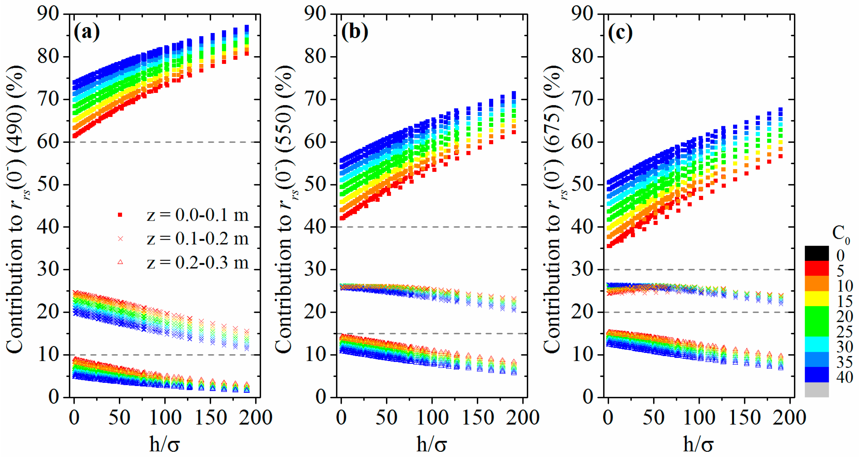
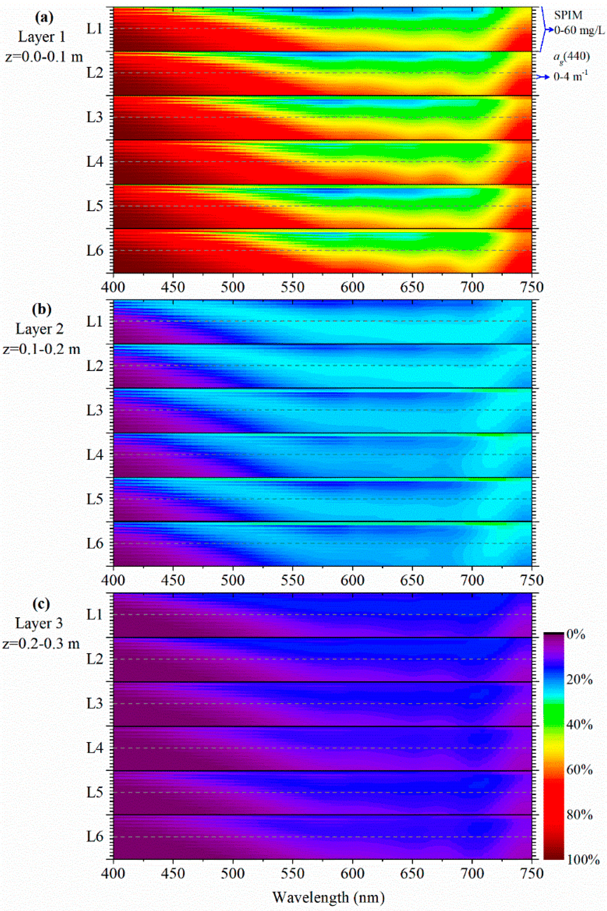
2.3. Contribution of Each Layer to r_rs(0⁻, λ)

In accordance with radiative transfer theory, Chla(z) profiles changed the AOPs(λ, z) of the underwater light field by modifying the IOP(λ, z) profiles. The relationship between the IOP(λ, z) of each layer and r_rs immediately below the water surface (r_rs(λ, 0⁻)) can be constructed through the K_x(λ, z) profiles based on the average weighting approach [8], and this relationship can then be used to calculate the contribution of each layer to the r_rs(λ, 0⁻).

The contribution of each layer between z₁ m and z₂ m to a remotely sensed signal can be derived using Equation (8) [10]:

$$Fr(z_1,z_2)={\displaystyle {\int }_{z_1}^{z_2}{IOP}^{\prime }}(z)\frac{d}{dz}[\exp \{-{\displaystyle {\int }_0^z[g_x(z^{\prime })]{dz}^{\prime }}\}]dz/{\displaystyle {\int }_0^{\infty }{IOP}^{\prime }}(z)\frac{d}{dz}[\exp \{-{\displaystyle {\int }_0^z[g_x(z^{\prime })]{dz}^{\prime }}\}]dz,$$

(8)

$${IOP}^{\prime }(z)=\frac{b_b(z)}{a(z)+b_b(z)},$$

(9)

where Fr(z₁, z₂) is the fraction of r_rs(λ, 0⁻) at the layer between z₁ m and z₂ m, g_x(z) is the average weighting function. Three weighting average functions, namely, g_GC [8], g_Z [10], and g_S [9], are as follows:

$$g_{GC}(\lambda ,z)=exp(-2{\displaystyle \underset{0}{\overset{z_{90}}{\int }}{K}_d(\lambda ,z^{\prime })}{dz}^{\prime }),$$

(10)

where z₉₀ is the depth at which 90% of the surface E_d(λ) has been attenuated.

$$g_Z(\lambda ,z)=2K_d(\lambda ,z)\exp (-2{\displaystyle \underset{0}{\overset{z}{\int }}{K}_d(\lambda ,z^{\prime })}{dz}^{\prime }),$$

(11)

where the depth dependence of g_Z is a function of the derivative of the round-trip attenuation of the downwelling and backscattering light. Gordon and Clark [8] stated that 2K_d(z) should be the sum of K_d(z) and K_Lu(z), hence K_d + K_Lu is also used to compare their performance with 2K_d in g_GC and g_Z.

$$\begin{array}{l}{g}_S(\lambda ,z)={\displaystyle {\int }_0^z{b}_{bd}(\lambda ,z)\exp \{-[K_d(\lambda ,\mathrm{z})+K_u(\lambda ,z)]\text{}}{dz}^{\prime }}\\ \approx {\displaystyle {\int }_0^z{K}_d(\lambda ,z)\exp [-3K_d(\lambda ,z)]{dz}^{\prime }}\end{array},$$

(12)

where b_bd is the diffuse backscattering coefficient, which is difficult to obtain. Thus, g_S is written as a function of K_d in the extreme case of b_b(z) $\propto$ K_d(z) [9].

To evaluate the performance of the model, the coefficient of correlations (R²) and the average absolute percentage difference (APD, %) were calculated to identify the difference between the simulated data (X_i) and the modeled data (Y_i).

$$\mathrm{APD}=\frac{1}{\mathrm{n}}{\displaystyle \sum _{\mathrm{i}=1}^{\mathrm{n}}\frac{\left|{\mathrm{Y}}_{\mathrm{i}}-{\mathrm{X}}_{\mathrm{i}}\right|}{{\mathrm{X}}_{\mathrm{i}}}}\times 100\%$$

(13)

3. Results

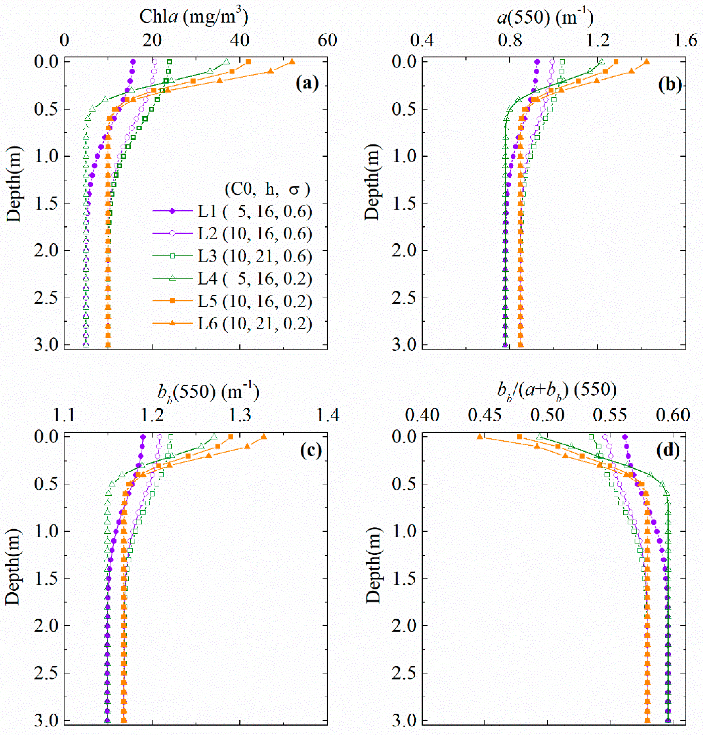
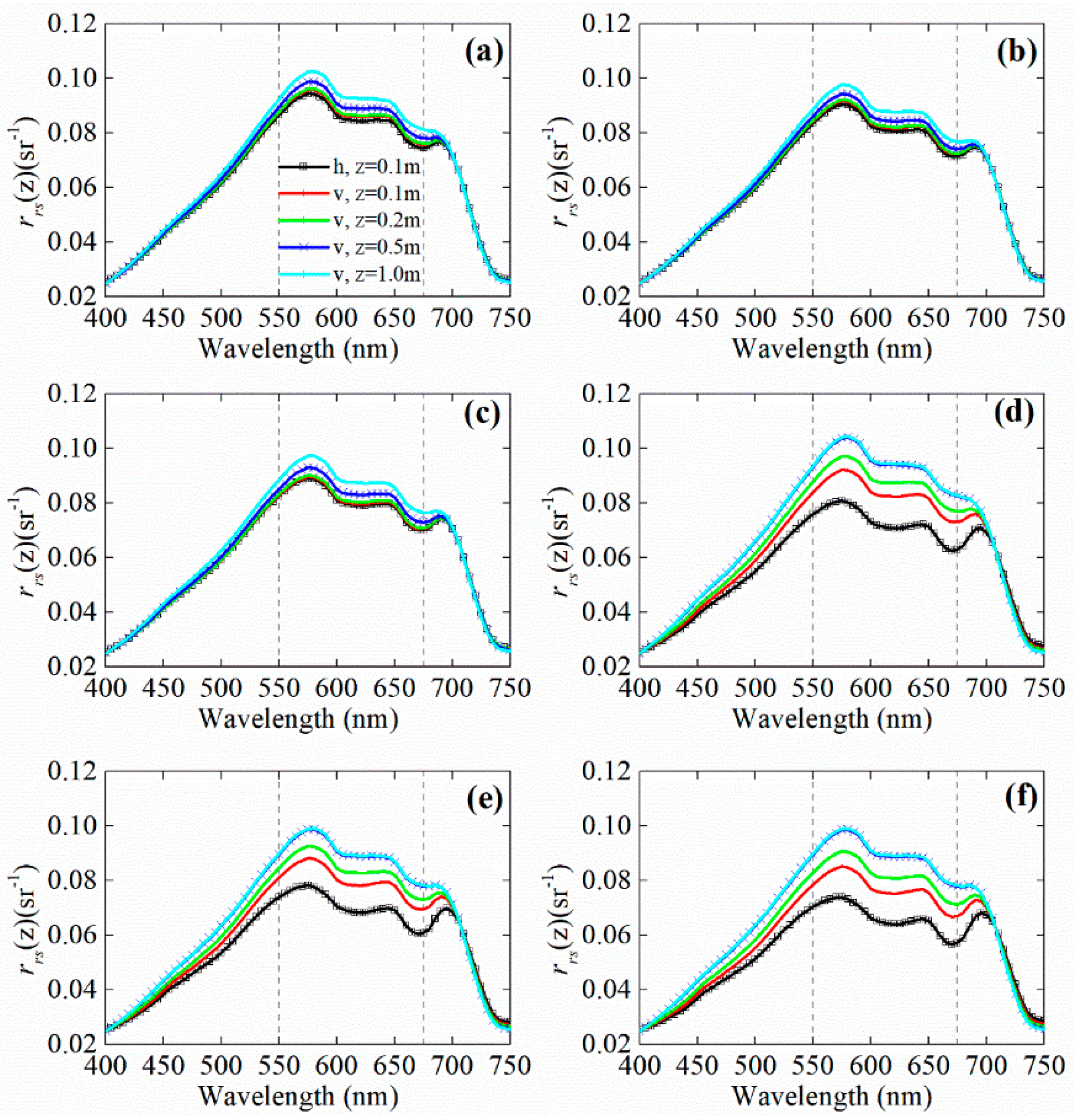
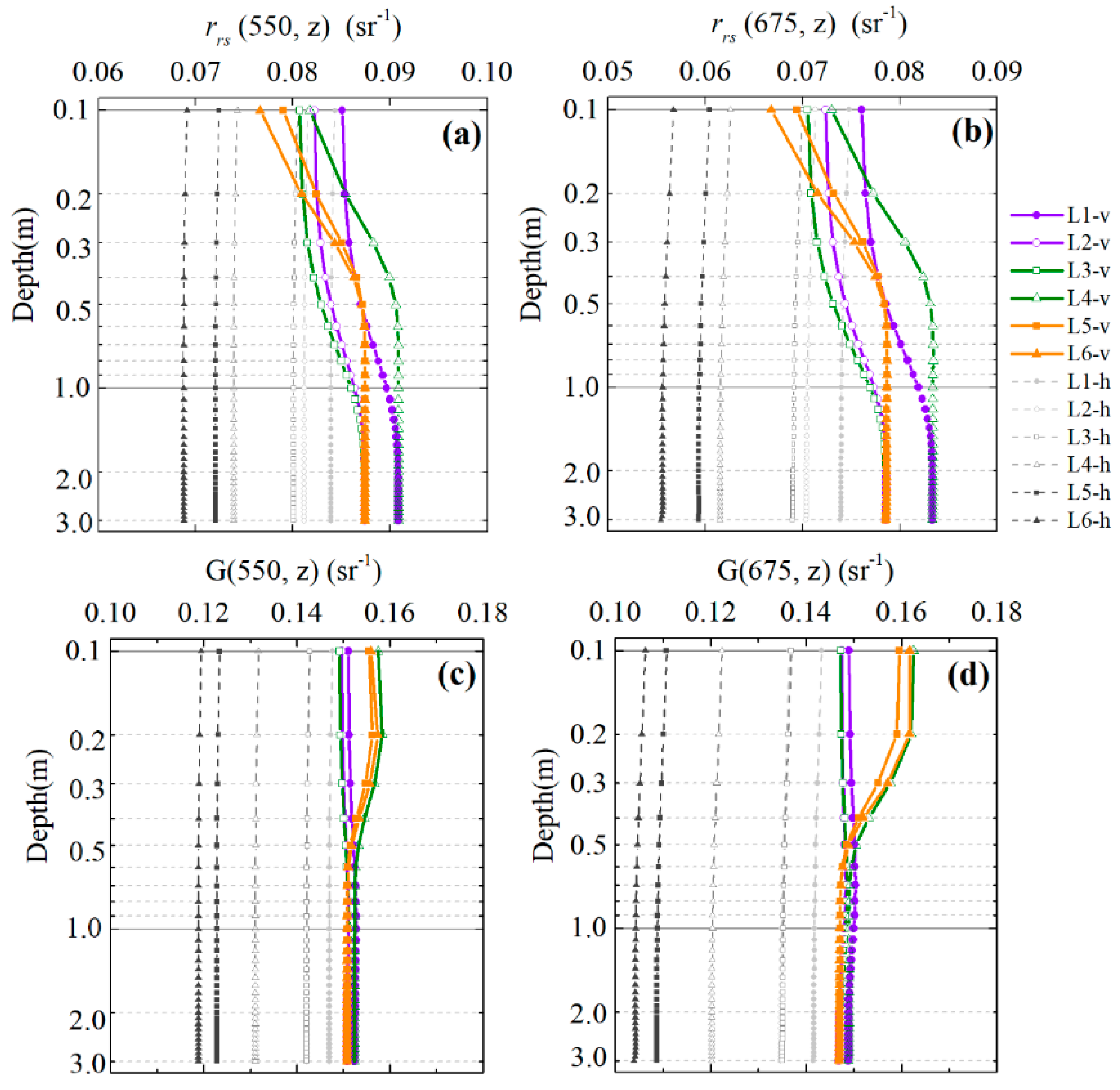
3.1. Effects of Chla(z) Profiles on r_rs(λ, z)

The six Chla(z) profiles (L1–L6, Figure 1) were used as examples to illustrate the spectral and vertical variations of r_rs(λ, z) in the vertical inhomogeneous waters (Figure 2 and Figure 3). In general, Chla(z) profiles changed the spectrum and magnitude of r_rs(λ, z) at different water depths. Compared with r_rs(λ, z) in homogeneous waters, r_rs(λ, z) considerably increased with water depth and reached the asymptotic value at a certain depth in which Chla(z) became unchangeable. In addition, the spectral variations of r_rs(λ, z) in seriously stratified waters were larger than that of Chla(z) profiles with less vertical variations. For example, the difference between r_rs(λ, z) at depth z and the asymptotic r_rs(λ, z_b) value (Δr_rs(λ, z)) of L3–L6 was noticeably larger than that of L1 and L2. Δr_rs(λ, z) exhibited spectral variations at the green and red wavelengths with a maximum value of approximately 590 nm and showed no evident spectrum shifting of the maximum value (Figure 2).

The vertical variations of r_rs(z) were also observed from profiles L1–L6 at 550 nm and 675 nm (Figure 3a,b). A large Δr_rs typically occurred at a depth in which Chla(z) exhibited large vertical variations. For example, L1 and L2 achieved the largest variations of Chla(z) and Δr_rs at the water depth between 0.5 m and 1.0 m, whereas L4 and L6 obtained the largest Δr_rs at the water depth between 0.2 m and 0.5 m. Δr_rs is also related to the vertical variation of Chla(z) profiles. For example, the difference of r_rs between 0.1 m and 0.2 m at 550 nm (Δr_rs(550, 0.1–0.2)) of L6 was 0.014 sr⁻¹, whereas the Δr_rs(550, 0.1–0.2) of L1 was close to 0.001 sr⁻¹. In general, Δr_rs(λ, z) increased with an increase in h and a decrease in σ and C₀. High h and low σ produce high vertical variation of Chla near the water surface, thereby leading to high Δr_rs(λ, z) (~78%) in L4 and L6. Moreover, the vertical Chla(z) profiles considerably affect r_rs(z) in low background concentration Chla (C₀). The Δr_rs between 0.1 m and 0.2 m of L5–L6 (C₀ = 5) was slightly larger than that of L3–L4 (C₀ = 10). That is, r_rs will vary substantially in relatively clear waters with large vertical variations of Chla(z).

The r_rs(λ, z) profiles exhibited a similar vertical trend with b_b/(a + b_b)(λ, z), but their ratio [G(λ, z) = r_rs(λ, z)/(b_b/(a + b_b)(λ, z))] varied depending on water depth (Figure 3c,d). G(λ, z) presented a slight increase in the first layer and then decreased with an increase in depth, particularly in L6 at 675 nm. However, G(λ, z) showed minimal vertical variation in cases with low vertical variation of Chla(z) profiles, such as in L1–L2. This indicated that G(λ, z) contains information of vertical variations between r_rs(λ, z) and b_b/(a + b_b)(λ, z), and the traditional bio-optical remote sensing model (Equation (1)) would not work in stratified waters. For example, b_b/(a + b_b)(675, 0⁻) of L5 is 0.535, the r_rs(675, 0⁻) would be 0.086 sr⁻¹(= 0.535*G(675, 0⁻)), but the r_rs(675, 0⁻) derived from Ecologht is 0.069 sr⁻¹. The absolute difference between r_rs(675, 0⁻) without considering vertical variations and Ecolight-derived r_rs(675, 0⁻) of L5 would be 24.6%.

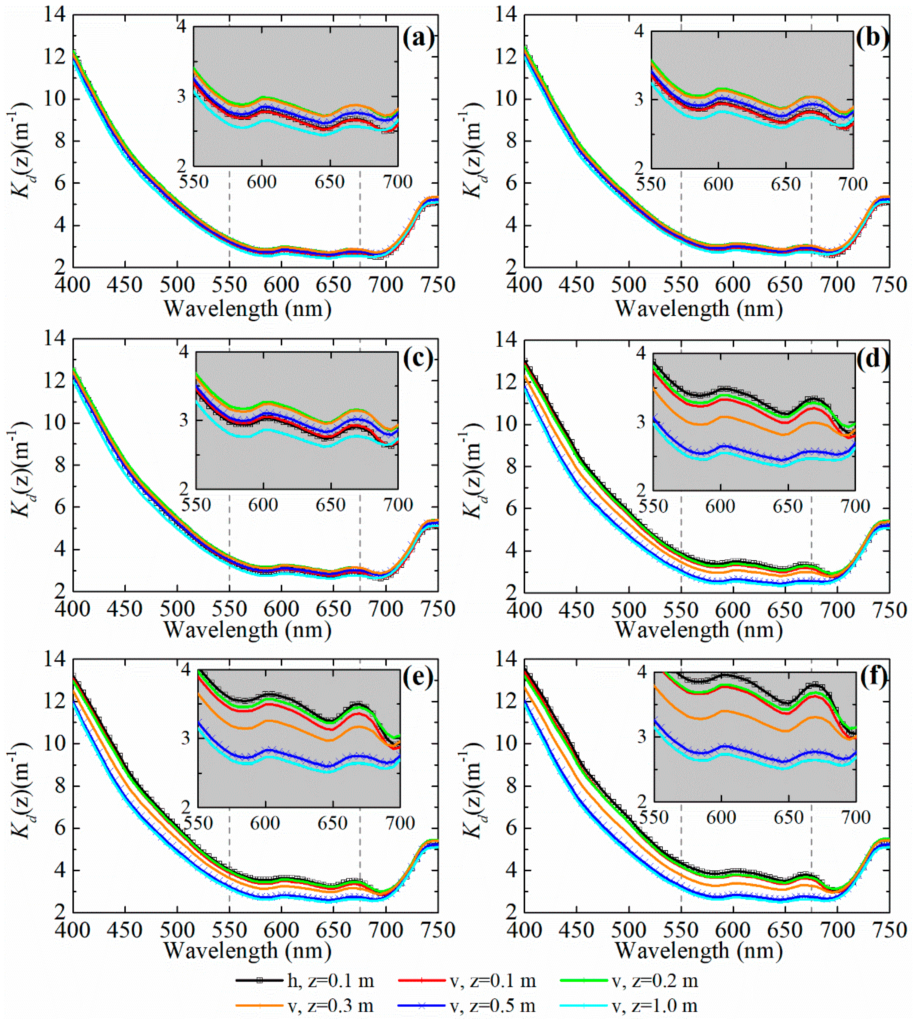
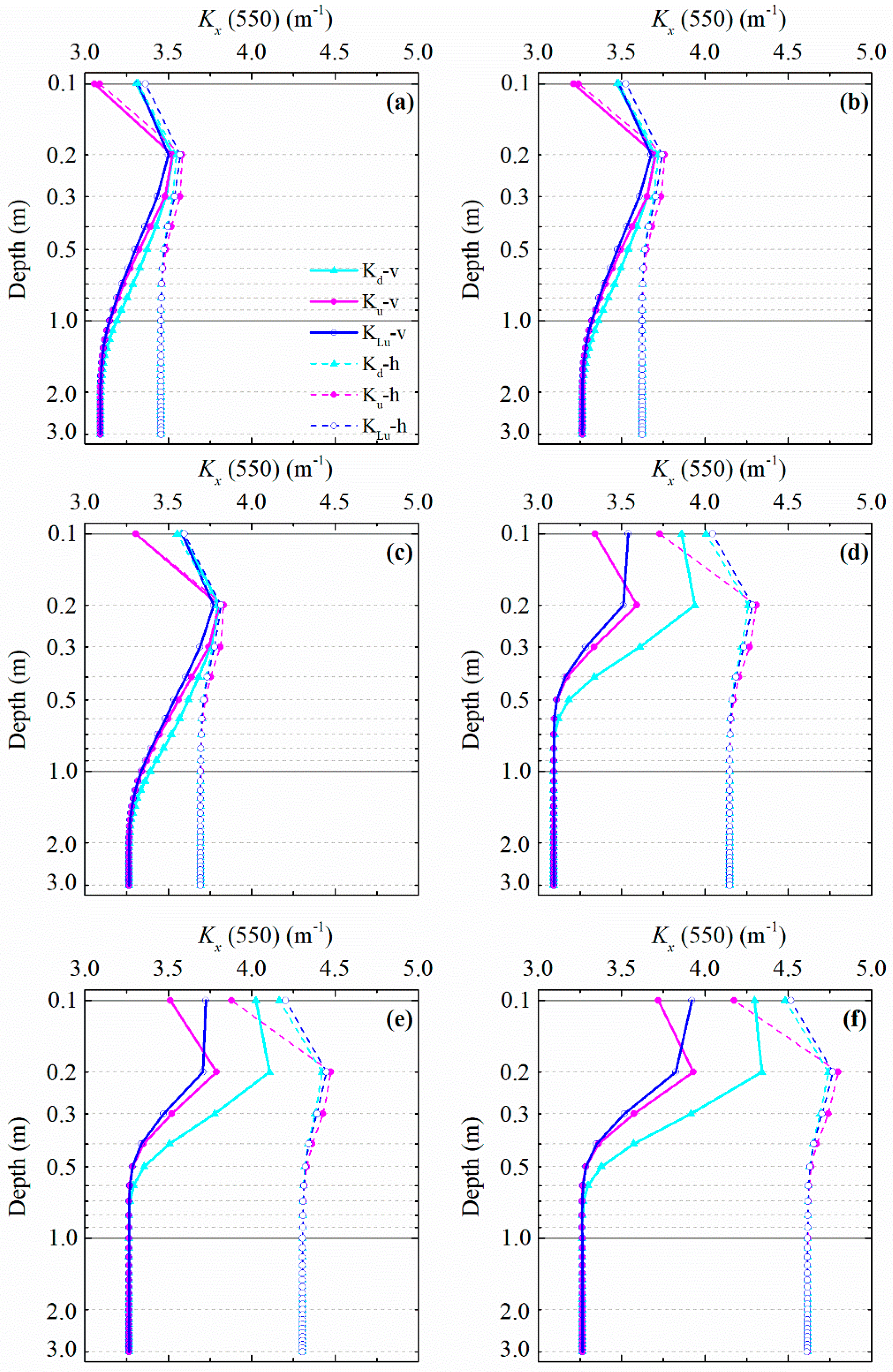
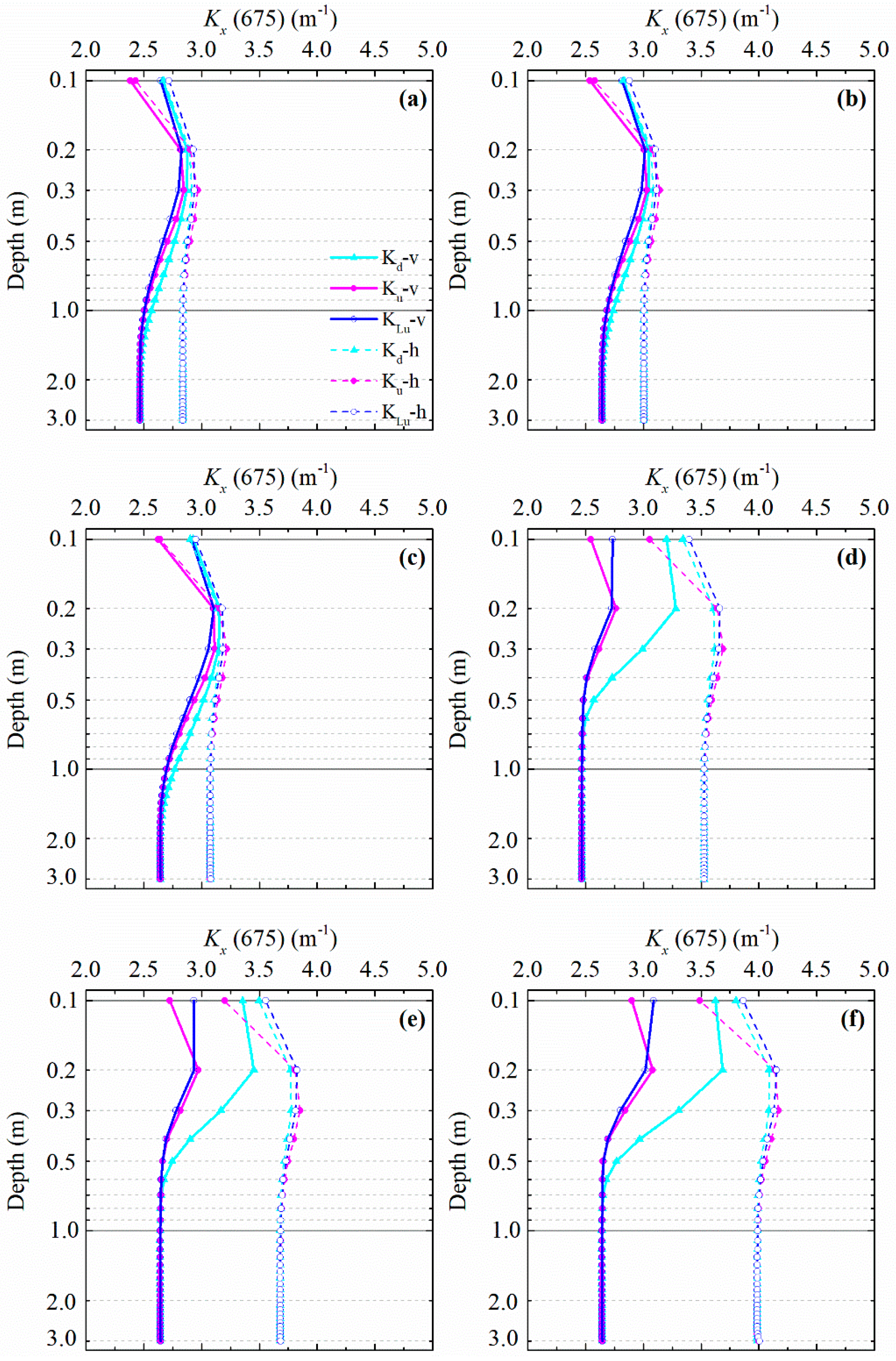
3.2. Effects of Chla(z) Profiles on K_x(λ, z)

The vertical distributions of Chla(z) also affected the spectral and vertical variations of K_x(λ, z) (Figure 4, Figure 5 and Figure 6). Similar to vertically homogeneous waters, K_d(λ, z) had a similar spectrum shape as K_u(λ, z) and K_Lu(λ, z), and K_x(λ, z) would reach the same asymptotic value when Chla(z) profiles became uniform at a great water depth. The K_d(λ, z) in the blue range was approximately thrice as that in the green and red bands due to the high content of phytoplankton, NAP, and CDOM (Figure 4a). K_d(λ, z) did not exhibit an evident spectral difference among different water depths with less vertical variation of Chla(z) (L1 and L2 in Figure 4a,b). However, K_d(λ, z) varied considerably from the blue to red wavelengths in seriously stratified waters (L4–L6 in Figure 4d–f). That is, the increase in Chla value at a certain depth added to the attenuation of this layer and increased K_x. The results showed that the K_d(λ, z) spectrum had highest values at z = 0.2 m in waters with low Chla(z) vertical variation, but had highest values at z = 0.1 m with large vertical discrepancy in stratified waters (Figure 4). In the highly stratified waters (L4–L6), K_d(λ, z) spectrum of deep water (e.g., z = 0.5, 1.0 m) showed weak spectral features in the range of 650 to 700 nm (Figure 4d–f).

The K_x(z) profiles at 550 and 675 nm in L1–L6 showed that K_d(λ, z) had larger vertical variations than K_u(λ, z) and K_Lu(λ, z) in highly stratified waters (Figure 5 and Figure 6). Note that the instability of K_x(λ, z) near water surface (z = 0.1 m) may be caused by the boundary conditions in the air–water surface. K_d(550, z) had minimal vertical variations and was slightly higher than K_u(550, z) and K_Lu(550, z) under conditions with less vertical variability (L1–L2). However, K_d(550, z) had higher value and larger vertical variability than K_u(550, z) and K_Lu(550, z) in L3–L6, thereby indicating that E_d(550, z) decreased more dramatically than E_u(550, z) and L_u(550, z) in these cases. Compared with the asymptotic value, the difference between K_x(550, z) at a depth of 0.2 m and the asymptotic K_x(550, z_b) value (ΔK_x(550)) in L6 was 1.59, 0.94, and 1.05 m⁻¹ for K_d, K_u, and K_Lu, respectively. In addition, compared with vertical homogeneous cases, K_x(550, z) and K_x(675, z) profiles were obvious lower, especially in highly stratified waters. In general, similar to Δr_rs(λ, z), ΔK_x(λ, z) increased with an increase in h, and decreased with the decrease of σ and C₀.

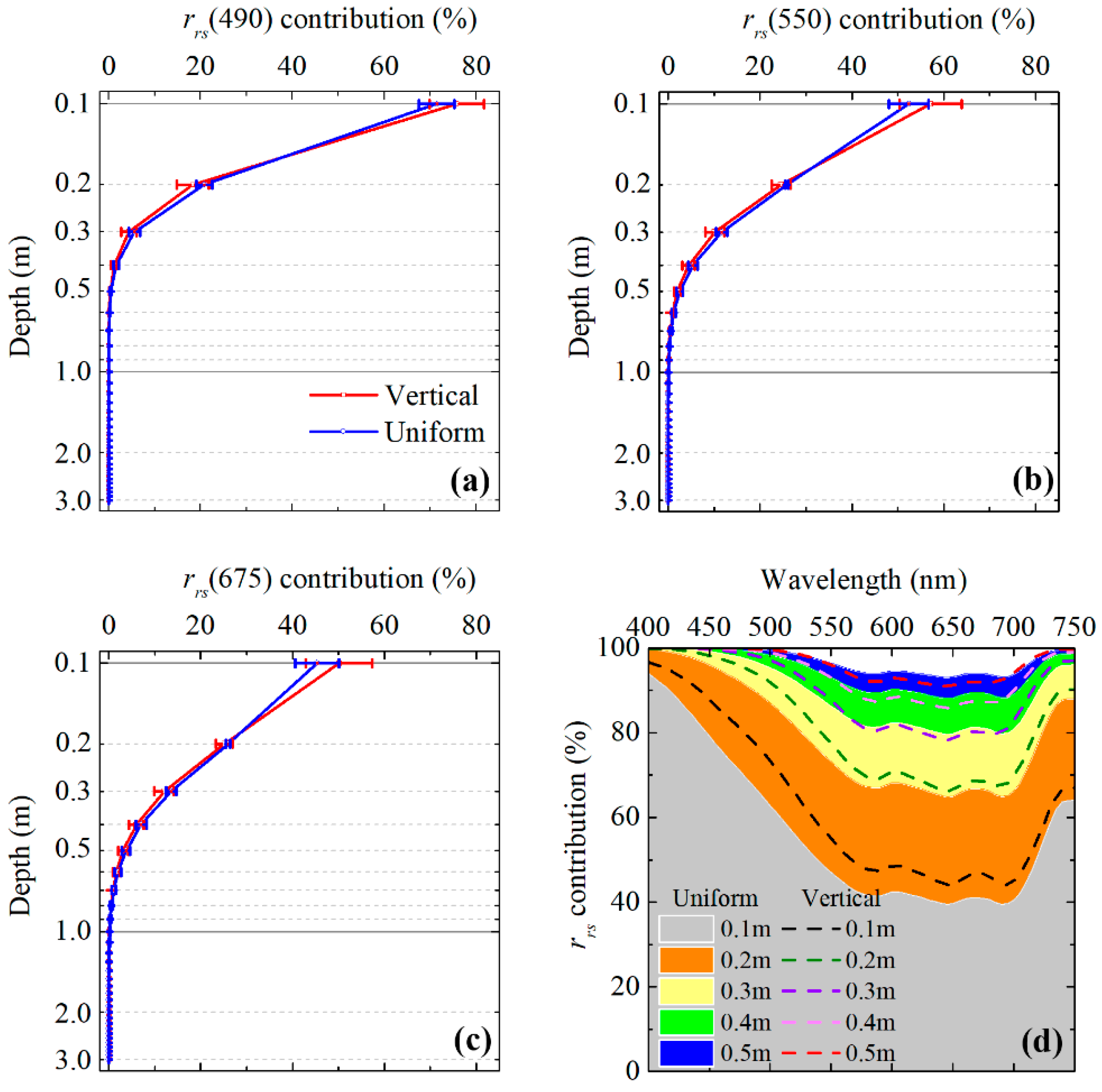
3.3. Contribution of Each Layer to r_rs(0⁻)

The contribution of each layer to r_rs(λ, 0⁻) can be derived using suitable average weighting functions and K_x(λ, z) profiles based on the average weighting theory. First, the three average weighting functions (i.e., g_GC, g_Z, and g_S, Equations (10)–(12)) were compared to select the g_x function with the best performance in our simulated data. K_d + K_Lu was compared with 2K_d in g_GC and g_Z due to the large difference between K_d(λ, z) and K_Lu(λ, z) in stratified waters. The results indicated that the combination of g_Z with K_d + K_Lu achieved relatively better performance in obtaining the weight-averaged r_rs(λ, 0⁻) (Figure 7a). Notably, the average relative error (RE) between the Ecolight-simulated and weight-averaged r_rs(λ, 0⁻) derived using g_Z(K_d + K_Lu) was low in 490 nm (~1.2%) and 550 nm (~0.9%), but obviously high in 675 nm (~7.8%). Among all the 1008 simulated data, data with RE < 2% contributed 82% (827/1008) and 90% (908/1008) in 490 nm and 550 nm, respectively; but data with RE > 10% were about 21% (208/1008) in 675 nm. Taking L1 as an example, the weight-averaged r_rs(λ, 0⁻) derived using the five weighting average functions were almost same with the Ecolight-simulated r_rs(λ, 0⁻), except the wavelength around 675 nm (Figure 7b). It indicated that Chla fluorescence affected the accuracy of average weighted r_rs(λ, 0⁻) around 675 nm. However, the weight-averaged r_rs(λ, 0⁻) showed a little departure from Ecolight-simulated r_rs(λ, 0⁻) in highly stratified waters (L4, L6), especially in the wavelength ranging from 550 nm to 700 nm (Figure 7c,d). The weight-averaged r_rs(λ, 0⁻) derived using g_Z(K_d + K_Lu) was considerably closer to the r_rs(λ, 0⁻) simulated by Ecolight in L6 (Figure 7d).

When g_Z(K_d + K_Lu) was used, the average contribution of each layer to r_rs(0⁻) at 490, 550, and 675 nm generally decreased with water depth and varied at different wavelengths (Figure 8a–c). Overall, layer 1 (0–0.1 m) contributed a noticeably larger budget to r_rs(0⁻) than the second layer (0.1–0.2 m) and the third (0.2–0.3 m), particularly within the blue range. In vertical inhomogeneous waters, the first layer contributed 75% and the second layer contributed 20% in the 490 nm; however, the first layer contributed 50% and the second layer contributed 25% in the 675 nm. That is to say, r_rs(0⁻) contained information from a certain depth, which also varied with wavelength. The contribution of each layer to the r_rs(0⁻) of L6 clearly showed the spectral differences at each layer (Figure 8d). The first two or three layers could dominate r_rs(0⁻) in the blue band, whereas 20% of the contribution would come from water deeper than 0.3 m in the L6 profile. The first two layers (z = 0–0.2 m) of L6 profile contributed more than the vertical uniform case, while, the first three layers (z = 0–0.3 m) had similar contribution in vertical inhomogeneous case and homogeneous case.

The contribution of the first three layers to r_rs(0⁻) were then related to the structure parameters (C₀, h/σ) of Chla(z) profiles (Figure 9). The contribution to r_rs(0⁻) increased with increasing h/σ in the first layer, but slightly decreased with increasing h/σ in the second and third layers. h/σ represents the vertical variation of Chla(z) near the water surface. When h/σ was high, Chla(z) would have noticeably higher value in the first layer, which increased the contribution of this layer. In addition, with increasing C₀, the background value of Chla in the column, the contribution of r_rs(0⁻) increased in the first layer but decreased in the second and third layers. The effects of the structure parameters of the Chla(z) profiles on r_rs contribution varied among different wavelengths and weakened in deep water.

Take the six Chla(z) profiles (L1–L6) as examples, the contribution of each layer to r_rs(0⁻) also varied with different SPIM (ranging from 0 to 60 mg/L) and a_g(440) (ranging from 0 to 4 m⁻¹) values (Figure 10). Compared with those of a_g(440), the variations of SPIM considerably influenced the contribution to r_rs(0⁻). In waters with low SPIM, L1 contributed lower than that in waters with high SPIM at the range of 550–700 nm. For example, the contribution of L1 to r_rs(0⁻) increased from 17% to 91% at 490 nm and from 16% to 72% at 550 nm with SPIM increasing from 0 to 60 mg/L. Meanwhile, the contribution of each layer to r_rs(0⁻) had low variations (~5%) with a_g(440) ranging from 0 to 4 m⁻¹, particularly when SPIM was high. Overall, the contribution of each layer to r_rs(0⁻) varied with water depth, wavelength, structure parameters of Chla(z) profiles, SPIM, and a_g(440). The contribution to r_rs(0⁻) varied from 30% to 85% in the first layer, ~10–25% in the second layer, and ~10% in the third layer. However, one important finding was that the contributions of the first two layers were approximately 80–90% to r_rs(0⁻) in these waters.

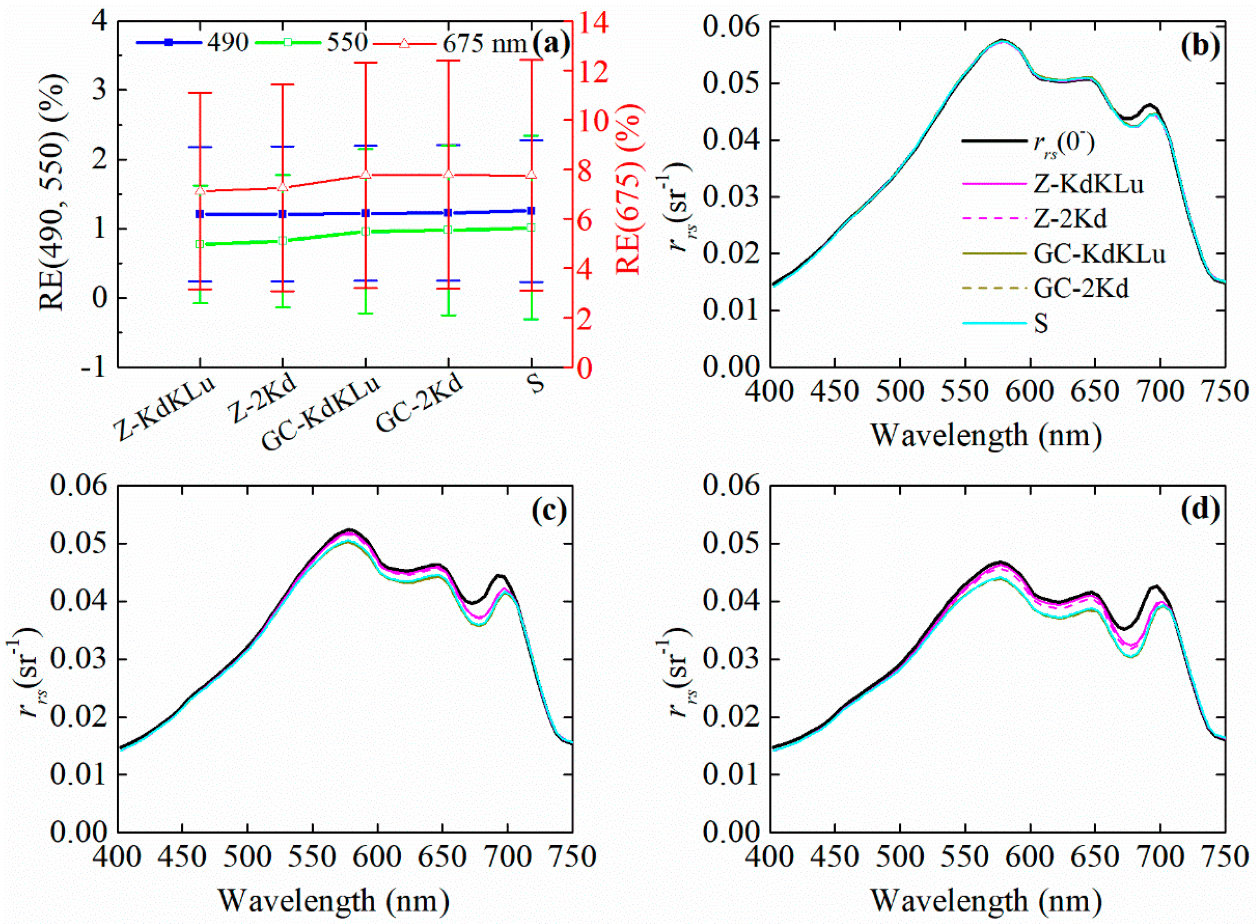
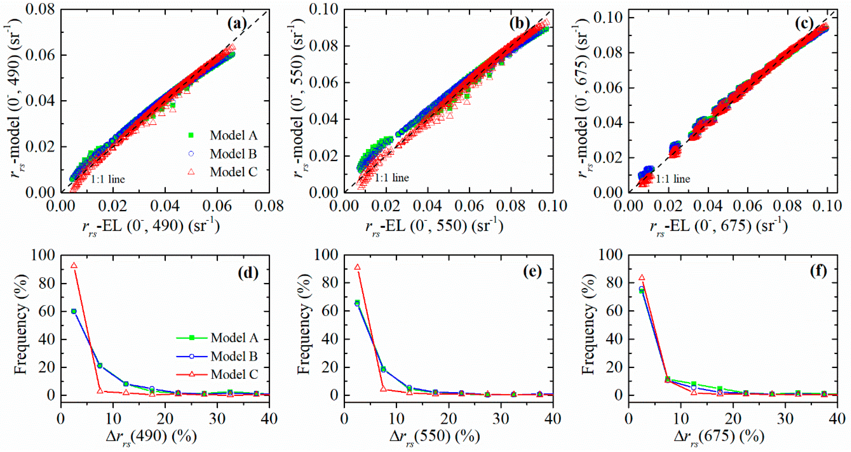
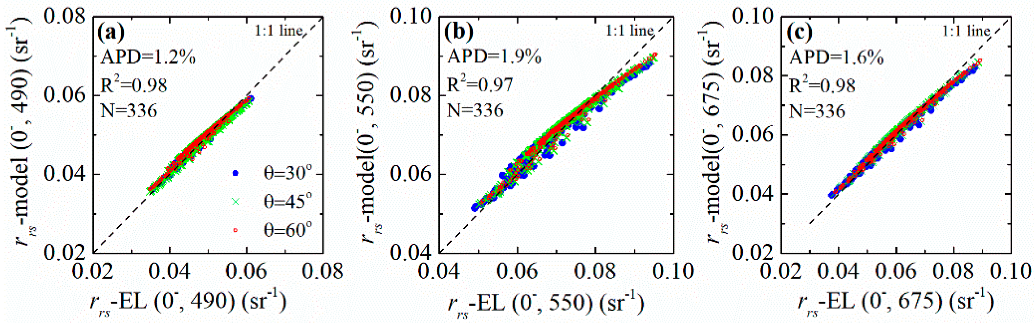
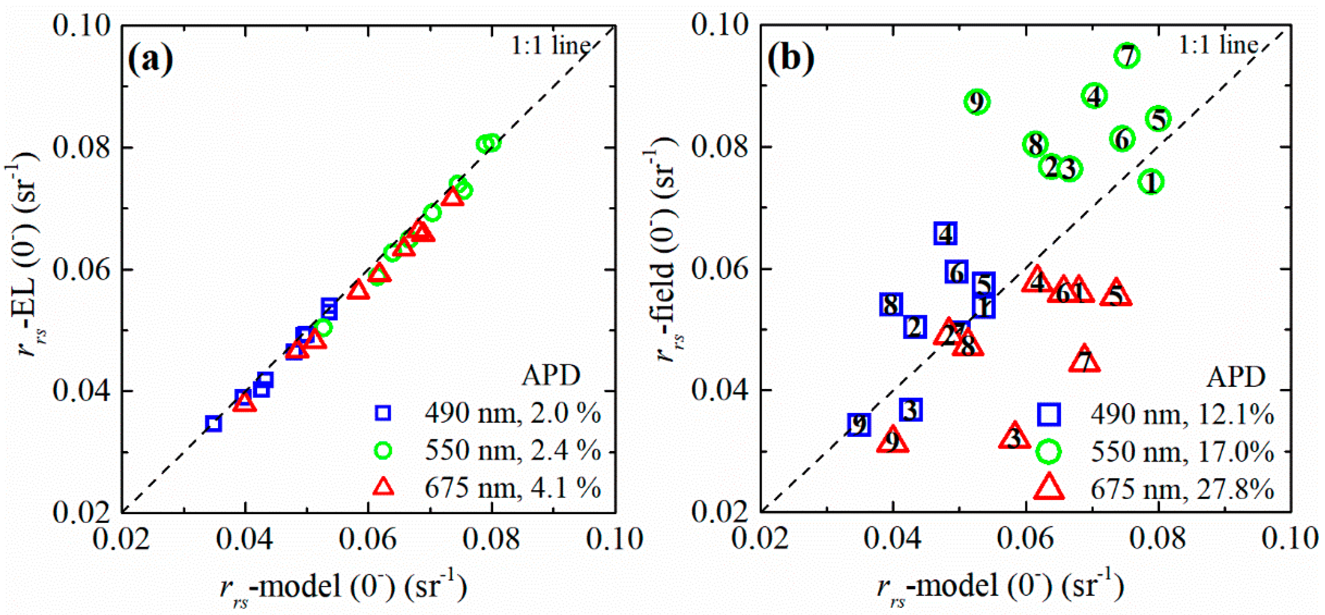
3.4. Remote Sensing Reflectance Model Considering Vertical Distribution Of Phytoplankton

The results of numerical simulations indicated that the traditional remote sensing reflectance model is insufficient for describing the relationship between r_rs(0⁻) and IOP′(z) in vertically inhomogeneous waters. In general, multiple g values (Equation (1)) will exist for the same IOP′(z = 0) value on the water surface with a vertical variation of phytoplankton. Based on weighting average theory and Equation (8), r_rs(0⁻) in vertically inhomogeneous waters (r_rs-v(0⁻)) can be related to IOP′(z), Fr(z), and g_x(z) of different water depths.

$$\begin{array}{l}{r}_{rs\text{-}v}(0^{-})={\displaystyle {\int }_0^{\infty }{IOP}^{\prime }}(z)\frac{d}{dz}[\exp \{-{\displaystyle {\int }_0^z[g_x(z^{\prime })]{dz}^{\prime }}\}]dz\\ ={\displaystyle \sum _{i=1}^{n-1}Fr(z_i,z_{i+1})\times {\displaystyle {\int }_{z_i}^{z_{i+1}}{IOP}^{\prime }}(z)\frac{d}{dz}[\exp \{-{\displaystyle {\int }_0^z[g_x(z^{\prime })]{dz}^{\prime }}\}]dz}\\ ={\displaystyle \sum _{i=1}^{n-1}{IOP}^{\prime }({\mathrm{z}}_{\mathrm{i}}\to {\mathrm{z}}_{\mathrm{i}+1})\times Fr(z_i,z_{i+1})\times {\displaystyle {\int }_{z_i}^{z_{i+1}}\frac{d}{dz}[\exp \{-{\displaystyle {\int }_0^z[g_x(z^{\prime })]{dz}^{\prime }}\}]dz}}\end{array},$$

(14)

where

$${IOP}^{\prime }(z_i\to z_{i+1})=\frac{b_b(\lambda ,z_i\to z_{i+1})}{a(\lambda ,z_i\to z_{i+1})+b_b(\lambda ,z_i\to z_{i+1})}.$$

(15)

By assuming

$$S_i=Fr(z_i,z_{i+1})\times {\displaystyle {\int }_{z_i}^{z_{i+1}}\frac{d}{dz}[\exp \{-{\displaystyle {\int }_0^z[g_x(z^{\prime })]{dz}^{\prime }}\}]dz},$$

(16)

r_rs–v(λ, 0⁻) can be written as the relationship between IOP’(λ, z) and parameter S_i(λ, z):

$$\begin{array}{l}{r}_{rs\text{-}v}(\lambda ,0^{-})={\displaystyle \sum _{i=1}^n[S_i(\lambda )\times {IOP}^{\prime }(\lambda ,z_i)}]\\ =S_1(\lambda )\times {IOP}^{\prime }(\lambda ,z_1)+S_2(\lambda )\times {IOP}^{\prime }(\lambda ,z_2)+\dots +S_{n-1}(\lambda )\times {IOP}^{\prime }(\lambda ,z_n)\end{array}.$$

(17)

As waters of the top 0.3 m contributed a large part of r_rs(0⁻) in the simulated data in Lake Chaohu; hence, a simple, stratified remote sensing model for nadir-viewed r_rs(0⁻) can be built based on Equation (17). Three simple models (Model A, Model B, and Model C) with polynomial expression were built using the absorption and backscattering coefficients of the first two or three layers. The model parameters (S_Ai, S_Bi, and S_Ci) of each model can be determined using the curve fitting toolbox in MATLAB R2015b.

Model A:

$$r_{rs\text{-}\mathrm{v}1}(\lambda ,0^{-})=S_{\mathrm{A}1}(\lambda ,z(1))\frac{b_b(\lambda ,z(1))}{a+b_b(\lambda ,z(1))}+S_{\mathrm{A}2}(\lambda ,z(2))\frac{b_b(\lambda ,z(2))}{a+b_b(\lambda ,z(2))}+S_{\mathrm{A}3}(\lambda ,z(3))\frac{b_b(\lambda ,z(3))}{a+b_b(\lambda ,z(3))}$$

(18)

Model B:

$$r_{rs\text{-}\mathrm{v}2}(\lambda ,0^{-})=S_{\mathrm{B}1}(\lambda ,z(1))\frac{b_b(\lambda ,z(1))}{a+b_b(\lambda ,z(1))}+S_{\mathrm{B}2}(\lambda ,z(2))\frac{b_b(\lambda ,z(2))}{a+b_b(\lambda ,z(2))}$$

(19)

Model C:

$$r_{rs\text{-}\mathrm{v}3}(\lambda ,0^{-})=S_{\mathrm{C}1}(\lambda ,z(1))\frac{b_b(\lambda ,z(1))}{a+b_b(\lambda ,z(1))}+S_{\mathrm{C}2}(\lambda ,z(2))\frac{b_b(\lambda ,z(2))}{a+b_b(\lambda ,z(2))}+S_{\mathrm{C}3}(\lambda )$$

(20)

A similar relative difference between modeled and simulated r_rs(0⁻) occurred in Models A and B, and approximately 20% of the calibration data had an average error of r_rs(0⁻) > 10% (Figure 11). The similar performance of Model A and Model B indicated that adding the contribution of waters between 0.2 m and 0.3 m did not improve the performance of Model A. When a constant term was added to the expression in Model C, the average difference would decrease to below 10%. Model C has a maximum error of ~3.5% and an average error of ~0.9% for nadir-viewed r_rs(0⁻) in this study. Therefore, for the given optical properties, Model C provided r_rs(0⁻) spectra that closely matched the theoretical values.

The parameters of Model C (i.e., S_C1, S_C2, and S_C3) were listed for five sun zenith angles (i.e., 15°, 30°, 45°, 60°, and 75°) and three wavelengths (i.e., 490, 550, and 675 nm) (

Table 3. Look up table of model parameters of Model C at different solar zenith angle (θ = 15°, 30°, 45°, 60°, and 75°) at 490, 550, and 675 nm.

θ (°)	Parameters	490 nm	550 nm	675 nm
	SC1	0.0978	0.0617	0.0758
15	SC2	0.0460	0.1041	0.0836
	SC3	−0.0068	−0.0123	−0.0067
	SC1	0.0998	0.0644	0.0791
30	SC2	0.0455	0.1023	0.0813
	SC3	−0.0067	−0.0120	−0.0065
	SC1	0.1034	0.0695	0.0848
45	SC2	0.0443	0.0983	0.0770
	SC3	−0.0064	−0.0114	−0.0060
	SC1	0.1050	0.0720	0.0879
60	SC2	0.0436	0.0961	0.0744
	SC3	−0.0062	−0.0110	−0.0058
	SC1	0.1063	0.0746	0.0907
75	SC2	0.0427	0.0930	0.0714
	SC3	−0.0059	−0.0104	−0.0054

). Notably, the parameters for various light geometries and wavelengths can also be developed, which can then be used to model r_rs(λ, 0⁻) over a wide range of optical properties. The proposed Model C was validated using the remaining 1/3 Ecolight-simulated data. A comparison between the Ecolight-simulated r_rs(0⁻) and the model-derived r_rs(0⁻) showed that the stratified r_rs model performed well, and only 1.43% of the validation data had APD of >5%. The average APD was 1.2%, 1.9%, and 1.6% at 490, 550, and 675 nm, respectively (Figure 12).

The Model C was then validated using the field-measured data (N = 9) in Lake Chaohu on 28 May 2013. The model parameters at 490, 550, and 675 nm were obtained from Table 3, according to the sampling location and time of each station. The measured Chla(z) profiles, SPIM, a_g(440), and SIOPs were set as the input parameters in Ecolight to derive the Ecolight-simulated r_rs(0⁻) of each sample. The comparison of model-derived r_rs(0⁻) and Ecolight-simulated r_rs(0⁻) indicated that Model C performed well with APD = 2.0%, 2.4%, and 4.1% at 490, 550, and 675 nm, respectively (Figure 13a). The model-derived r_rs(0⁻) was then compared with field-measured r_rs(0⁻), which was derived from field-measured R_rs(λ) using the Equation (21) [47].

$$r_{rs}(0^{-},\lambda )=R_{rs}(\lambda )/(0.52+1.7R_{rs}(\lambda )).$$

(21)

The results showed that acceptable relative errors were acquired when validating using the field-measured data (Figure 13). The APD of model-derived r_rs(0⁻) and field-measured r_rs(0⁻) was 12.1%, 17.0%, and 27.8% at 490, 550, and 675 nm, respectively (Figure 13b). The uncertainties may come from the difficulty in optical closure between Ecolight simulation and field measurement of natural waters, the measurement of R_rs(λ), and the derivation of r_rs(0⁻) from measured R_rs(λ).

4. Discussion

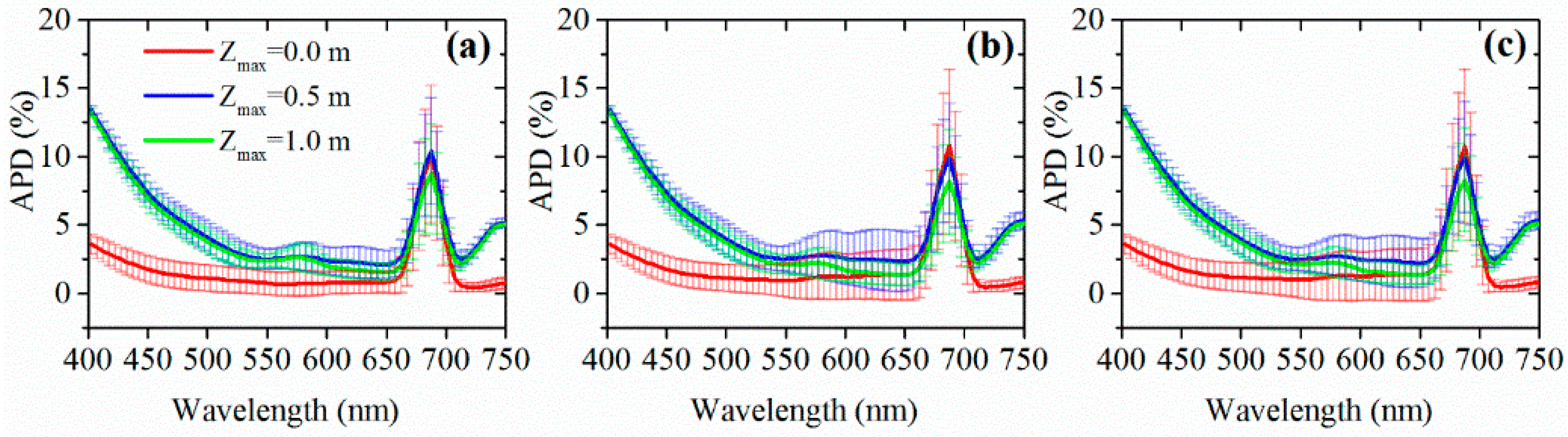
4.1. Performance of Weighting Average Functions

The stratified r_rs model was developed by evaluating the weighting average functions and calculating the contribution of each layer to r_rs(0⁻). If the weighting average function did not perform well, the contribution of each layer to r_rs(0⁻) (Equation (8)) and the modeled r_rs(0⁻) would be invalid. In the present study, five combinations of weighting average functions and K_x indicated that g_Z(K_d + K_Lu) achieved the best performance, whereas g_GC and g_S did not perform well, particularly in the green and red wavelengths in highly stratified waters (Figure 7). Moreover, Piskozub et al. [48] demonstrated that g_GC did not perform well in oceanic waters due to too much weight on the surface layer. The result in this study was also in accordance with the study of Gordon and Clark [8], in which the use of 2K_d instead of K_d + K_Lu in the weighting functions led to minimal errors only (<1%).

Gaussian function with maximum values in the water column is often used to describe Chla(z) profiles in oceanic waters and deep lakes:

$$\mathrm{Chl}a(\mathrm{z})={\mathrm{C}}_0+\frac{h}{\sigma \sqrt{2\pi }}\exp [-\frac{1}{2}{(\frac{z-z_{\max }}{\sigma })}^2].$$

(22)

To discuss the applicability of the stratified r_rs model in waters with different maximum Chla depths (Z_max = 0.0, 0.5, and 1.0 m), the performance of the three weighting average functions (g_Z-KdKLu, g_GC-KdKLu, g_S) in waters was compared (Figure 14). Evidently, g_Z-KdKLu had lower APD (<5%) than those of g_GC-KdKLu and g_S in Chla(z) profiles with maximum Chla at water surface Z_max = 0.0 m. However, these weighting functions performed worse in waters with maximum Chla under water surface Z_max > 0 m than Z_max = 0.0 m. For example, APD increased dramatically when Z_max = 0.5 m and 1.0 m, particularly in the blue spectrum (>10%). The APD in the case of Z_max = 1.0 m was slightly lower than that of Z_max = 0.5 m, thereby indicating that the effects of Chla(z) vertical profiles on R_rs could be weakened with an increase in Z_max. Overall, the performance of g_Z(K_d + K_Lu) in waters with different Z_max values verified that the weighting average functions are suitable to shallow eutrophic waters with Z_max = 0.0 m, but fail in waters with a deep Chla maximum layer [49].

K_d(λ, z) is very high in the blue region because of the rapid attenuation due to the high content of phytoplankton, NAP, and CDOM in this study. The magnitude and spectrum shape of K_d(λ, z) in this study is accordance with the previous studies in turbid productive waters [50,51,52]. However, K_d(λ, z) has low value in the blue region, and increases to high values in the red and NIR wavelength in clear waters [53,54]. The relatively high values of K_d(λ, z) in the red and NIR region results from the increasing absorption coefficients of pure water in these regions. Note that relatively large error was obvious in the wavelength ranging from 650 nm to 700 nm when calculating the contribution of each layer to r_rs(0⁻) (Figure 7) and evaluating the performance of weighting average functions (Figure 14). Owing to the large difference of attenuation rate between excitation and emission photons of inelastic scattering, inelastic scattering plays a greater role for the underwater light field at red wavelengths as depth increases [55]. One possible reason comes from the Chla fluorescence by changing the radiance field around 685 nm in the water column [56]. Similar to the previous study [55], K_d(λ, z) was spectral flat at deeper water depth (Figure 4). Note that the difference in spectral of K_x(λ, z) between different water depths added the errors of weighting average functions. In addition, it demonstrated that the inelastic processes produce strong depth dependence of the K_Lu(λ, 0⁻) in the red and NIR (near Infra-red) spectral regions within the near surface layer even within an optically homogeneous water column [56]. That is, the inelastic scattering in the red and NIR wavelength also contributes the uncertainties when using K_x(λ, z) in the weighting average functions to model the r_rs(0⁻) in vertical inhomogeneous waters. Due to the complex influence of inelastic scattering in underwater light field, we used the default model of inelastic scattering, and did not take the variations of inelastic scattering into consideration.

4.2. Limitations

A simple stratified remote sensing reflectance model considering Chla(z) vertical distribution was tested to illustrate the relationships between r_rs(0⁻) and IOP′(λ, z) with vertical variations. This model related r_rs(0⁻) to absorption and backscattering coefficients, and used model parameters, varying in wavelength and sun zenith angle, to express the relationship between IOP′(λ, z) of the top two layers (z = 0–0.1 m and 0.1–0.2 m) and r_rs(0⁻) in stratified waters. One limitation is that this model is suitable for eutrophic lakes with maximum Chla value on the water surface. The Ecolight simulation was processed based on field measurement in Lake Chaohu, a shallow eutrophic lake with frequently occurring algal blooms. Under self-regulation and appropriate environmental conditions (e.g., temperature, light, and wind), algae typically accumulate on the water surface and exhibit vertical inhomogeneous distribution with the maximum Chla value on the water surface [7]. Moreover, the performance of this model depends on the accuracy of weighting average functions; hence, one huge challenge in its further application is developing appropriate and accurate weighting functions for waters with different vertical distribution types. Another limitation is that SPIM and CDOM were assumed to be vertically uniform based on the field data of Lake Chaohu. However, SPIM and CDOM do not covary with phytoplankton and may not be vertically uniform in natural waters. Thus, attention should be directed on the different vertical structures of phytoplankton, sediments, and CDOM in Case 2 waters [10]; and it is common that they are distribute irregularly in the natural waters.

5. Conclusions

The vertical variation of IOPs characterized by Chla(z) vertical profiles with maximum value on the water surface (shifted Gaussian function) frequently occurs in shallow eutrophic waters. However, current remote sensing reflectance algorithms typically do not consider the vertical structure of Chla(z) profiles. Radiative transfer simulations of underwater light field with different vertical profiles of Chla(z) indicated that vertical variations of phytoplankton considerably affected AOPs, e.g., r_rs(λ, z) and K_x(λ, z), which are key parameters to describe the underwater light field. The vertical distribution of Chla(z) profiles changed the spectrum shape and magnitude of r_rs(λ, z) and K_x(λ, z). The substantial vertical variation of the underwater light field occurs at water depths with large vertical variations of Chla(z) profiles. Differences in r_rs(λ) between the vertical non-uniform and asymptotic values can reach 78%, particularly when the Chla(z) profiles decreases dramatically with low σ or high h. In addition, the contribution of the first three layers to r_rs(λ, 0⁻) was approximately 90%, but the contribution of each layer varied with wavelength, the structure parameters of Chla(z) profiles, SPIM, and CDOM. As an implication, a stratified remote sensing reflectance model was developed based on the contribution of each layer to r_rs(λ, 0⁻) to understand the relationship between r_rs(λ, 0⁻) and IOP’(λ, z). To apply the model to other types of waters, accurate weighting average functions and validation based on large radiative transfer simulation dataset and field-measured data are necessary. Nevertheless, the proposed remote sensing reflectance model has the potential to be used in developing water color remote sensing models in inhomogeneous waters.

References

1. Odermatt, D.; Pomati, F.; Pitarch, J.; Carpenter, J.; Kawka, M.; Schaepman, M.; Wüest, A. MERIS observations of phytoplankton blooms in a stratified eutrophic lake. Remote Sens. Environ. 2012, 126, 232–239. [Google Scholar] [CrossRef]
2. Bresciani, M.; Adamo, M.; De Carolis, G.; Matta, E.; Pasquariello, G.; Vaičiūtė, D.; Giardino, C. Monitoring blooms and surface accumulation of cyanobacteria in the Curonian Lagoon by combining MERIS and ASAR data. Remote Sens. Environ. 2014, 146, 124–135. [Google Scholar] [CrossRef]
3. Millán-Núñez, R.; Alvarez-Borrego, S.; Trees, C.C. Modeling the vertical distribution of chlorophyll in the California Current System. J. Geophys. Res. 1997, 102, 8587. [Google Scholar] [CrossRef]
4. André, J.-M. Ocean color remote-sensing and the subsurface vertical structure of phytoplankton pigments. Deep Sea Res. Part A Oceanogr. Res. Pap. 1992, 39, 763–779. [Google Scholar] [CrossRef]
5. Forget, P.; Broche, P.; Naudin, J.-J. Reflectance sensitivity to solid suspended sediment stratification in coastal water and inversion: A case study. Remote Sens. Environ. 2001, 77, 92–103. [Google Scholar] [CrossRef]
6. Nanu, L.; Robertson, C. The effect of suspended sediment depth distribution on coastal water spectral reflectance: Theoretical simulation. Int. J. Remote Sens. 1993, 14, 225–239. [Google Scholar] [CrossRef]
7. Xue, K.; Zhang, Y.; Duan, H.; Ma, R.; Loiselle, S.; Zhang, M. A Remote Sensing Approach to Estimate Vertical Profile Classes of Phytoplankton in a Eutrophic Lake. Remote Sens. 2015, 7, 14403–14427. [Google Scholar] [CrossRef] [Green Version]
8. Gordon, H.R.; Clark, D.K. Remote sensing optical properties of a stratified ocean: An improved interpretation. Appl. Opt. 1980, 19, 3428–3430. [Google Scholar] [CrossRef]
9. Sokoletsky, L.G.; Yacobi, Y.Z. Comparison of chlorophyll a concentration detected by remote sensors and other chlorophyll indices in inhomogeneous turbid waters. Appl. Opt. 2011, 50, 5770–5779. [Google Scholar] [CrossRef]
10. Zaneveld, J.R.V.; Barnard, A.; Boss, E. Theoretical derivation of the depth average of remotely sensed optical parameters. Opt. Express 2005, 13, 9052–9061. [Google Scholar] [CrossRef]
11. Duan, H.; Ma, R.; Zhang, Y.; Loiselle, S.A.; Xu, J.; Zhao, C.; Zhou, L.; Shang, L. A new three-band algorithm for estimating chlorophyll concentrations in turbid inland lakes. Environ. Res. Lett. 2010, 5, 044009. [Google Scholar] [CrossRef] [Green Version]
12. Song, K.; Li, L.; Tedesco, L.P.; Li, S.; Duan, H.; Liu, D.; Hall, B.E.; Du, J.; Li, Z.; Shi, K.; et al. Remote estimation of chlorophyll-a in turbid inland waters: Three-band model versus GA-PLS model. Remote Sens. Environ. 2013, 136, 342–357. [Google Scholar] [CrossRef]
13. Duan, H.; Ma, R.; Hu, C. Evaluation of remote sensing algorithms for cyanobacterial pigment retrievals during spring bloom formation in several lakes of East China. Remote Sens. Environ. 2012, 126, 126–135. [Google Scholar] [CrossRef]
14. Song, K.; Li, L.; Li, Z.; Tedesco, L.; Hall, B.; Shi, K. Remote detection of cyanobacteria through phycocyanin for water supply source using three-band model. Ecol. Inform. 2013, 15, 22–33. [Google Scholar] [CrossRef]
15. Kutser, T.; Metsamaa, L.; Strömbeck, N.; Vahtmäe, E. Monitoring cyanobacterial blooms by satellite remote sensing. Estuar. Coast. Shelf Sci. 2006, 67, 303–312. [Google Scholar] [CrossRef]
16. Zhang, Y.; Ma, R.; Zhang, M.; Duan, H.; Loiselle, S.; Xu, J. Fourteen-Year Record (2000–2013) of the Spatial and Temporal Dynamics of Floating Algae Blooms in Lake Chaohu, Observed from Time Series of MODIS Images. Remote Sens. 2015, 7, 10523–10542. [Google Scholar] [CrossRef] [Green Version]
17. Gordon, H.R.; McCluney, W. Estimation of the depth of sunlight penetration in the sea for remote sensing. Appl. Opt. 1975, 14, 413–416. [Google Scholar] [CrossRef] [PubMed]
18. Tsujimura, S.; Tsukada, H.; Nakahara, H.; Nakajima, T.; Nishino, M. Seasonal variations of Microcystis populations in sediments of Lake Biwa, Japan. Hydrobiologia 2000, 434, 183–192. [Google Scholar] [CrossRef]
19. Stramska, M.; Stramski, D. Effects of a nonuniform vertical profile of chlorophyll concentration on remote-sensing reflectance of the ocean. Appl. Opt. 2005, 44, 1735–1747. [Google Scholar] [CrossRef] [PubMed]
20. Kutser, T.; Metsamaa, L.; Dekker, A.G. Influence of the vertical distribution of cyanobacteria in the water column on the remote sensing signal. Estuar. Coast. Shelf Sci. 2008, 78, 649–654. [Google Scholar] [CrossRef]
21. Xue, K.; Zhang, Y.; Ma, R.; Duan, H. An approach to correct the effects of phytoplankton vertical nonuniform distribution on remote sensing reflectance of cyanobacterial bloom waters. Limnol. Oceanogr. Methods 2017, 15, 302–319. [Google Scholar] [CrossRef]
22. Silulwane, N.F.; Richardson, A.J.; Shillington, F.A.; Mitchell-Innes, B.A. Identification and classification of vertical chlorophyll patterns in the Benguela upwelling system and Angola-Benguela front using an artificial neural network. S. Afr. J. Mar. Sci. 2010, 23, 37–51. [Google Scholar] [CrossRef]
23. Mobley, C.D. Light and Water: Radiative Transfer in Natural Waters; Academic Press: Cambridge, MA, USA, 1994; pp. 155–162. [Google Scholar]
24. Sundarabalan, B.; Shanmugam, P.; Ahn, Y.H. Modeling the underwater light field fluctuations in coastal oceanic waters: Validation with experimental data. Ocean Sci. J. 2016, 51, 67–86. [Google Scholar] [CrossRef]
25. Gordon, H.R. Ship perturbation of irradiance measurements at sea. 1: Monte Carlo simulations. Appl. Opt. 1985, 24, 4172–4182. [Google Scholar] [CrossRef] [PubMed]
26. Kirk, J.T.O. Monte Carlo study of the nature of the underwater light field in, and the relationships between optical properties of, turbid yellow waters. Mar. Freshw. Res. 1981, 32, 517–532. [Google Scholar] [CrossRef]
27. Morel, A.; Gentili, B. Diffuse reflectance of oceanic waters: Its dependence on Sun angle as influenced by the molecular scattering contribution. Appl. Opt. 1991, 30, 4427–4438. [Google Scholar] [CrossRef]
28. Plass, G.N.; Kattawar, G.W. Radiative Transfer in an Atmosphere-Ocean System. Appl. Opt. 1969, 8, 455–466. [Google Scholar] [CrossRef]
29. Jin, Z.; Stamnes, K. Radiative transfer in nonuniformly refracting layered media: Atmosphere-ocean system. Appl. Opt. 1994, 33, 431–442. [Google Scholar] [CrossRef]
30. Chami, M.; Lafrance, B.; Fougnie, B.; Chowdhary, J.; Harmel, T.; Waquet, F. OSOAA: A vector radiative transfer model of coupled atmosphere-ocean system for a rough sea surface application to the estimates of the directional variations of the water leaving reflectance to better process multi-angular satellite sensors data over the ocean. Opt. Express 2015, 23, 27829–27852. [Google Scholar] [CrossRef]
31. Chami, M.; Santer, R.; Dilligeard, E. Radiative transfer model for the computation of radiance and polarization in an ocean–atmosphere system: Polarization properties of suspended matter for remote sensing. Appl. Opt. 2001, 40, 2398–2416. [Google Scholar] [CrossRef]
32. He, X.; Bai, Y.; Zhu, Q.; Gong, F. A vector radiative transfer model of coupled ocean–atmosphere system using matrix-operator method for rough sea-surface. J. Quant. Spectrosc. Radiat. Transf. 2010, 111, 1426–1448. [Google Scholar] [CrossRef]
33. Ramon, D.; Steinmetz, F.; Jolivet, D.; Compiègne, M.; Frouin, R. Modeling polarized radiative transfer in the ocean-atmosphere system with the GPU-accelerated SMART-G Monte Carlo code. J. Quant. Spectrosc. Radiat. Transf. 2019, 222–223, 89–107. [Google Scholar] [CrossRef]
34. Zhai, P.-W.; Hu, Y.; Chowdhary, J.; Trepte, C.R.; Lucker, P.L.; Josset, D.B. A vector radiative transfer model for coupled atmosphere and ocean systems with a rough interface. J. Quant. Spectrosc. Radiat. Transf. 2010, 111, 1025–1040. [Google Scholar] [CrossRef]
35. Zhai, P.-W.; Hu, Y.; Winker, D.M.; Franz, B.A.; Werdell, J.; Boss, E. Vector radiative transfer model for coupled atmosphere and ocean systems including inelastic sources in ocean waters. Opt. Express 2017, 25, A223–A239. [Google Scholar] [CrossRef] [PubMed]
36. Ota, Y.; Higurashi, A.; Nakajima, T.; Yokota, T. Matrix formulations of radiative transfer including the polarization effect in a coupled atmosphere–ocean system. J. Quant. Spectrosc. Radiat. Transf. 2010, 111, 878–894. [Google Scholar] [CrossRef]
37. Zaneveld, J.R.V. A theoretical derivation of the dependence of the remotely sensed reflectance of the ocean on the inherent optical properties. J. Geophys. Res. Oceans 1995, 100, 13135–13142. [Google Scholar] [CrossRef]
38. Morel, A.; Gentili, B. Diffuse reflectance of oceanic waters. II Bidirectional aspects. Appl. Opt. 1993, 32, 6864–6879. [Google Scholar] [CrossRef]
39. Gordon, H.R.; Brown, O.B.; Evans, R.H.; Brown, J.W.; Smith, R.C.; Baker, K.S.; Clark, D.K. A semianalytic radiance model of ocean color. J. Geophys. Res. Atmos. 1988, 93, 10909–10924. [Google Scholar] [CrossRef]
40. Lee, Z.; Carder, K.L.; Du, K. Effects of molecular and particle scatterings on the model parameter for remote-sensing reflectance. Appl. Opt. 2004, 43, 4957–4964. [Google Scholar] [CrossRef]
41. Pitarch, J.; Odermatt, D.; Kawka, M.; Wuest, A. Retrieval of vertical particle concentration profiles by optical remote sensing: A model study. Opt. Express 2014, 22 (Suppl. 3), A947–A959. [Google Scholar] [CrossRef]
42. Gitelson, A.A.; Dall’Olmo, G.; Moses, W.; Rundquist, D.C.; Barrow, T.; Fisher, T.R.; Gurlin, D.; Holz, J. A simple semi-analytical model for remote estimation of chlorophyll-a in turbid waters: Validation. Remote Sens. Environ. 2008, 112, 3582–3593. [Google Scholar] [CrossRef]
43. Werdell, P.J.; Franz, B.A.; Bailey, S.W.; Feldman, G.C.; Boss, E.; Brando, V.E.; Dowell, M.; Hirata, T.; Lavender, S.J.; Lee, Z.; et al. Generalized ocean color inversion model for retrieving marine inherent optical properties. Appl. Opt. 2013, 52, 2019–2037. [Google Scholar] [CrossRef] [Green Version]
44. Jiang, G.; Ma, R.; Loiselle, S.A.; Duan, H. Optical approaches to examining the dynamics of dissolved organic carbon in optically complex inland waters. Environ. Res. Lett. 2012, 7, 034014. [Google Scholar] [CrossRef] [Green Version]
45. Cao, Z.; Duan, H.; Feng, L.; Ma, R.; Xue, K. Climate- and human-induced changes in suspended particulate matter over Lake Hongze on short and long timescales. Remote Sens. Environ. 2017, 192, 98–113. [Google Scholar] [CrossRef]
46. Xue, K.; Zhang, Y.; Duan, H.; Ma, R. Variability of light absorption properties in optically complex inland waters of Lake Chaohu, China. J. Great Lakes Res. 2017, 43, 17–31. [Google Scholar] [CrossRef]
47. Lee, Z.; Carder, K.L.; Arnone, R.A. Deriving inherent optical properties from water color: A multiband quasi-analytical algorithm for optically deep waters. Appl. Opt. 2002, 41, 5755–5772. [Google Scholar] [CrossRef]
48. Piskozub, J.; Neumann, T.; Woźniak, L. Ocean color remote sensing: Choosing the correct depth weighting function. Opt. Express 2008, 16, 14683–14688. [Google Scholar] [CrossRef]
49. Latasa, M.; Cabello, A.M.; Massana, R.; Scharek, R. Distribution of phytoplankton groups within the deep chlorophyll maximum. Limnol. Oceanogr. 2016, 62, 635–638. [Google Scholar] [CrossRef]
50. Simon, A.; Shanmugam, P. A new model for the vertical spectral diffuse attenuation coefficient of downwelling irradiance in turbid coastal waters: Validation with in situ measurements. Opt. Express 2013, 21, 30082–30106. [Google Scholar] [CrossRef] [PubMed]
51. Simon, A.; Shanmugam, P. Estimation of the spectral diffuse attenuation coefficient of downwelling irradiance in inland and coastal waters from hyperspectral remote sensing data: Validation with experimental data. Int. J. Appl. Earth Obs. Geoinf. 2016, 49, 117–125. [Google Scholar] [CrossRef]
52. Wang, M.; Son, S.; Harding, L.W., Jr. Retrieval of diffuse attenuation coefficient in the Chesapeake Bay and turbid ocean regions for satellite ocean color applications. J. Geophys. Res. Oceans 2009, 114. [Google Scholar] [CrossRef] [Green Version]
53. Mishra, D.R.; Narumalani, S.; Rundquist, D.; Lawson, M. Characterizing the vertical diffuse attenuation coefficient for downwelling irradiance in coastal waters: Implications for water penetration by high resolution satellite data. ISPRS J. Photogramm. Remote Sens. 2005, 60, 48–64. [Google Scholar] [CrossRef]
54. Niroumand-Jadidi, M.; Pahlevan, N.; Vitti, A. Mapping Substrate Types and Compositions in Shallow Streams. Remote Sens. 2019, 11, 262. [Google Scholar] [CrossRef]
55. Zheng, X.; Dickey, T.; Chang, G. Variability of the downwelling diffuse attenuation coefficient with consideration of inelastic scattering. Appl. Opt. 2002, 41, 6477–6488. [Google Scholar] [CrossRef] [PubMed]
56. Li, L.; Stramski, D.; Reynolds, R.A. Effects of inelastic radiative processes on the determination of water-leaving spectral radiance from extrapolation of underwater near-surface measurements. Appl. Opt. 2016, 55, 7050–7067. [Google Scholar] [CrossRef] [PubMed]
Figure 1. Bio-optical properties of six representative examples: (a) Chla(z), (b) a(550), (c) bb(550), and (d) bb/(a + bb)(550). Different lines represent different vertical structure parameters (C0, h, σ) of Chla(z) profiles: L1 (5, 16, 0.6), L2 (10, 16, 0.6), L3 (10, 21, 0.6), L4 (5, 16, 0.2), L5 (10, 16, 0.2), L6 (10, 21, 0.2).
Applsci 09 01635 g001
Figure 2. rrs(z) spectrum of Chla(z) profiles: (a) L1 (5, 16, 0.6), (b) L2 (10, 16, 0.6), (c) L3 (10, 21, 0.6), (d) L4 (5, 16, 0.2), (e) L5 (10, 16, 0.2), and (f) L6 (10, 21, 0.2) at different water depths (z = 0.1, 0.2, 0.5, 1.0 m). “h” represents that the Chla value was vertical homogeneous, and the water depth is 0.1 m. “v” represents the vertical inhomogeneous cases. rrs(z) profiles at 550 and 675 nm (grey dash lines) shown in Figure 3a,b.
Applsci 09 01635 g002
Figure 3. rrs(λ, z) of Chla(z) vertical profiles (L1–L6) at (a) 550 and (b) 675 nm. G(λ, z) of Chla(z) vertical profiles (L1–L6) at (c) 550 and (d) 675 nm. Different lines represent different vertical structure parameters (C0, h, σ) of Chla(z) profiles: L1 (5, 16, 0.6), L2 (10, 16, 0.6), L3 (10, 21, 0.6), L4 (5, 16, 0.2), L5 (10, 16, 0.2), and L6 (10, 21, 0.2). The grey dashed lines represent the corresponding homogeneous cases of the vertical profiles (L1–L6).
Applsci 09 01635 g003
Figure 4. Kd(z) spectrum of Chla(z) profiles: (a) L1 (5, 16, 0.6), (b) L2 (10, 16, 0.6), (c) L3 (10, 21, 0.6), (d) L4 (5, 16, 0.2), (e) L5 (10, 16, 0.2), and (f) L6 (10, 21, 0.2) at different water depths (z = 0.1, 0.2, 0.3, 0.5, 1.0 m). The inserted figures showed the Kd(λ, z) in the range of 550 nm to 700 nm of each Chla(z) profiles. “h” represents that the Chla value was vertical homogeneous, and the water depth is 0.1 m. “v” represents the vertical inhomogeneous cases. Kd vertical profiles at 550 and 675 nm (grey dash lines) were showed in Figure 5 and Figure 6, respectively.
Applsci 09 01635 g004
Figure 5. Kx(550) vertical profiles under different Chla(z) distributions: (a) L1 (5, 16, 0.6), (b) L2 (10, 16, 0.6), (c) L3 (10, 21, 0.6), (d) L4 (5, 16, 0.2), (e) L5 (10, 16, 0.2), and (f) L6 (10, 21, 0.2). Kx represents Kd, Ku, and KLu. The solid lines represent the Kx(550, z) profiles in vertical inhomogeneous waters (“v”); the dashed lines represent the corresponding cases in vertical homogeneous waters (“h”).
Applsci 09 01635 g005
Figure 6. Kx(675) vertical profiles under different Chla(z) distributions: (a) L1 (5, 16, 0.6), (b) L2 (10, 16, 0.6), (c) L3 (10, 21, 0.6), (d) L4 (5, 16, 0.2), (e) L5 (10, 16, 0.2), and (f) L6 (10, 21, 0.2) at 550 nm. Kx represents Kd, Ku, and KLu. The solid lines represent the Kx(675, z) profiles in vertical inhomogeneous waters (“v”); the dashed lines represent the corresponding cases in vertical homogeneous waters (“h”).
Applsci 09 01635 g006
Figure 7. Performance of the five combinations of weighting average functions and Kx. (a) Average relative error of all the simulated data at 490, 550, and 675 nm. Note that 490 nm and 550 nm use the left axis, and 675 nm uses the right axis. Weighting averaged rrs of (b) L1 (5, 16, 0.6), (c) L4 (10, 16, 0.2), and (d) L6 (10, 21, 0.2) derived by the five weighting average functions. “Z-KdKLu” represents the approach of Zaneveld et al. (2005) using Kd + KLu in the weighting average function, “Z-2Kd” represents the approach of Zaneveld et al. (2005) using 2Kd, “GC-KdKLu” represents the approach of Gordon and Clark (1992) using Kd + KLu, “GC-2Kd” represents the approach of Gordon and Clark (1992) using 2Kd, and “S” represents the approach of Sokoletsky and Yacobi (2011).
Applsci 09 01635 g007
Figure 8. Average contribution of each layer to rrs of simulated data in vertical nonuniform (N = 1008) and uniform waters (N = 1008) at (a) 490, (b) 550, and (c) 675 nm. (d) Take L6 as an example, stacked rrs contribution of different layers in vertical nonuniform and uniform waters. The dashed lines represent the cases of vertical inhomogeneous water.
Applsci 09 01635 g008
Figure 9. Contribution of each layer to rrs(0) on different vertical structure parameters (C0, h/σ) at z = 0.1, 0.2, 0.3 m: (a) 490 nm, (b) 550 nm, (c) 675 nm. It indicated that the first three layers would contribute about 90% to rrs(0).
Applsci 09 01635 g009
Figure 10. Contribution of each layer to rrs(λ, 0) at different values of SPIM (0–60 mg/L with an interval of 5 mg/L, increasing from top to bottom in each large grid) and ag(440) (0–4 m−1 with an interval of 0.5 m−1, increasing from top to bottom in each small grid) in the wavelength region from 400 to 750 nm. Layer 1 is the water depth between 0.0 and 0.1 m; Layer 2 is the water depth between 0.1 and 0.2 m; Layer 3 is the water depth between 0.2 and 0.3 m. The grey dashed lines represent the cases with average SPIM and ag(440) values.
Applsci 09 01635 g010
Figure 11. Performances of Model A, Model B, and Model C: (ac) comparisons between modeled rrs(0) and Ecolight-simulated rrs(0) at 490, 550, and 675 nm, respectively; (df) frequency of Δrrs(0) of different models at 490, 550, and 675 nm, respectively.
Applsci 09 01635 g011
Figure 12. Validation of stratified rrs model using Ecolight-simulated data at (a) 490 nm, (b) 550 nm, and (c) 675 nm at different sun zenith angles (θ = 30°, 45°, 60°), respectively.
Applsci 09 01635 g012
Figure 13. Validation of stratified rrs model using field-measured data (N = 9) of Lake Chaohu on May 28, 2013. Comparison of rrs-model(0) with (a) Ecolight-simulated rrs-EL(0), and (b) field-measured rrs-field(0) at 490, 550, and 675 nm. Note that the model parameters were obtained from Table 3 according to the sampling time and location.
Applsci 09 01635 g013
Figure 14. Performance of weighting average functions: (a) gZ-KdKLu, (b) gGC-KdKLu, and (c) gS on Ecolight-simulated data with different maximum depth (Zmax) of Chla profiles.
Applsci 09 01635 g014