Abstract
This article aims to determine the most suitable cross-sectional area for a high voltage alternating current (HVAC) submarine cable in the design phase of new projects. A thermal ladder network method (LNM) was used to analyse the thermal behaviour in the centre of the conductor as the hottest spot of the cable. On the basis of the calculated cable parameters and a thermal cable analysis of transient conditions applied by a step function with a time duration greater than 1 h, this article proposes a method for a dynamic rating of submarine cables. The dynamic rating is accomplished through an iterative process. The method was tested with a MATLAB simulation and validated in comparison with a finite element method (FEM)-based approach.
1. Introduction
It has not always been as challenging as it is today to match energy generation levels with consumers’ power consumption patterns. Energy sources based on fossil fuels are being replaced by renewable power generation, such as wind energy, to reach one of the global climate goals of achieving at least a 27% share of renewable energy by 2030 [1]. Therefore, it is essential to investigate methods to reduce the cost associated with the transmission of renewable power generation. Multiple studies have discussed the application of Dynamic Line Rating (DLR) forecasting to already constructed lines to optimise transmission capacity [2,3]. The market for renewable power generation is growing fast, and the number and size of offshore wind farms have increased rapidly in the past several years. According to the Global Wind Energy Council, the annual installed global wind energy capacity has increased from 6.5 GW in 2001 to 52.4 GW in 2017 [4]. The disadvantage of such renewable power generation is the uncontrollability, as the power production varies with the speed of the wind. In order to carry massive amounts of power through a submarine cable (shown in Figure 1) connecting an offshore renewable power generation source, such as a wind farm, to an onshore station and simultaneously minimise the levelised energy costs (LEC) [5], it is essential to select the most suitable cable for each specific case. A way to achieve this is to change the design phase and dynamically rate cables on the basis of a worst-case estimation of varying load profiles and surrounding conditions (shown in Figure 1) of different cable environments. Such changing variables include burial depth L, thermal soil resistivity and ambient temperature .
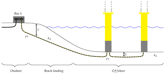
Figure 1.
Submarine cable installations between onshore grid (Bus 1) and wind turbine generator (WTG) foundations illustrating surrounding conditions: onshore, at the beach landing and offshore.
High voltage alternating current (HVAC) submarine cables are developed to carry a great amount of power across the water. The cable conductors consist of copper (Cu) or aluminium (Al), depending on size and price. Cross-linked polyethene (XLPE), with a maximum operational temperature of 90 C, is a commonly used insulation material. A common construction of a three-core XLPE separate lead (SL), sheath-type submarine cable is shown in Figure 2, where the internal part of the cable contains : Conductor, : Conductor screen, : Insulation, : Insulation screen, : Swelling tape, : Metallic sheath/screen, : Anti-corrosion sheath and the common covering, containing : Bedding, : Armour and : Outer serving. The element is the optical fibre used for communication and distributed temperature sensing (DTS) [6], and represents the fillers, which are usually filled with water while in operation.
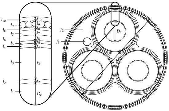
Figure 2.
General structure of a three-core cross-linked polyethene (XLPE) separate lead (SL)-type submarine cable with all layers included; diameters D, thickness t and layers l are illustrated and labelled.
The static rating of HVAC cables can be calculated by using a series of standards from the International Electrotechnical Commission named IEC 60287 [4] and has been historically conservative as it is based on worst-case assumptions and does not take into account real-time changes of surrounding conditions [7].
Renewable power generation such as wind energy delivers an unpredictable production profile that varies from no- to full-load several times within 24 h. In Figure 3, a typical current profile from a wind farm in Denmark is shown. By considering the thermal behaviour caused by the production variation, the cable parameters can be designed according to the actual load, which is the peak value of the actual flowing current , instead of using the steady-state rated current . Rating cables to conduct the actual current is performed through a thermal cable behaviour analysis, proposed in IEC 60853-2 [8]. This way, the selection of cable parameters can be improved, which can result in an economic advantage in the development phase [5]. Thermal considerations of offshore submarine cables are worthy of investigation, as the thermal soil conditions are better than those onshore. Thus, there is an excellent opportunity to utilise the surrounding conditions in the cable current rating phase.
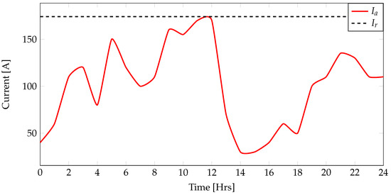
Figure 3.
Example of a current profile to illustrate rating issues, where is the actual current and is the current used for static rating.
Previous work has shown that on the basis of a more dynamic approach, a significant improvement in the transmission ability of cables can be achieved using real-time monitoring systems on existing cables, such as DTS [6]. This opens opportunities to investigate possibilities to use a dynamic cable rating method in the design phase of new projects.
2. Dynamic Cable Rating
Dynamic rating of cables, as the main focus of this paper, involves rating cables considering variable cable loading. It is an iterative method that comprises calculating electrical and thermal parameters on the basis of the IEC 60287 series [4] and conducting a thermal cable analysis according to IEC 60853-2 [8]. The method can be used for AC cables with a voltage above 36 kV, as defined by IEC 60853-2 [8]. In order to find an analytical solution for heat transfer from the centre of the conductor to the surface of the cable and take into account the impact of the surroundings, a thermal ladder network is built up to represent the electrical parameters of the cable and accordingly evaluate the transient temperature response by a step function.
Figure 4 is a simplified overview of the iterative method. The first stage is to determine an initial cable to design, and the second stage, which is detailed in Section 2.2, involves the determination of cable loading and electrical and thermal parameters. The third process, explained in Section 2.3, evaluates the transient temperature behaviour in the centre of the conductor on the basis of the electrical and thermal parameters determined in Section 2.2. The first decision box represents the iterative process of assessing the transient temperature response on the basis of the applied step function. With the usage of XLPE as insulation, the upper boundary is at 90 C. If the cable temperature is not within the temperature tolerance, a new cable is selected. The fifth stage represents the output of a suitable cable according to dynamic cable rating.
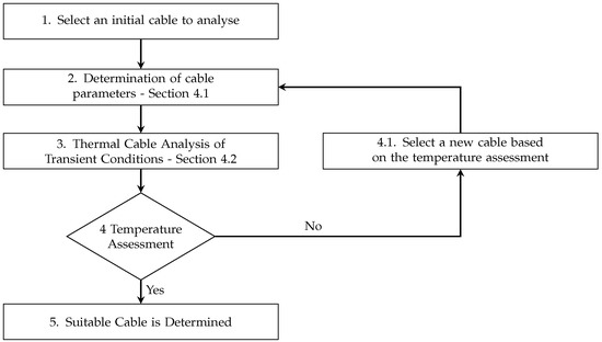
Figure 4.
Flowchart of the iterative dynamic cable rating method.
2.1. Thermal-Electrical Analogy for Cables
To model a ladder network consisting of thermal parameters, analogical thermal and electrical parameters must be determined. This section walks through the modelling of a thermal ladder network representing a three-core XLPE submarine cable and defines the thermal parameters. Insulation materials other than XLPE can be used if the cable structure is equivalent to the cable illustrated in Figure 2. The IEC 60287 series [4] and IEC 60853-2 [8] describe the electrical and thermal properties of the most common insulation materials. The electrical properties of a cable are often represented by infinite small sections of lumped parameters containing resistance and reactance in series and two capacitances C divided into two equal parts in parallel [9]. To represent the properties thermally, the electrical reactance X is neglected since it is the resistance R of the cable that determines the voltage drop and the capacitance C that defines the time constant of the voltage. Comparing the electrical model shown in Figure 5 and the thermal analogy of Figure 6, we can conclude proportionality between voltage V and temperature ; current I and heat flow w; electrical resistance R and thermal resistance T; electrical capacitance C and thermal capacitance Q.
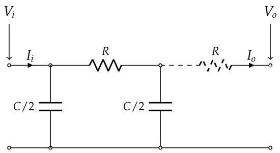
Figure 5.
Electrical analogy for cables.
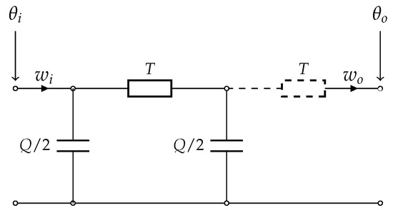
Figure 6.
Thermal analogy for cables.
The IEC 60853-2 [8] considerations of thermal analogies were written at the time when oil–paper cables were used; this means that the computation of a thermal ladder network does not represent a modern submarine cable with high accuracy. To represent the thermal properties of a three-core XLPE submarine cable with asymmetry between the internal and external parts of the cable and a lot of non-conductive layers, it is necessary to split the physical objects of the cable into small parts and represent each of them with thermal resistance and thermal capacitance. The thermal resistance represents the ability of the material to impede heat flow, and the thermal capacitance is defined as the ability to store heat [8]. This method is only applicable in cases where thermal parameters do not change as a function of temperature variations, because it solves heat flow equations using the superposition principle, which is used exclusively for linear systems.
2.2. Determination of Cable Parameters
Thermal and electrical parameters are used to perform a temperature analysis and are calculated according to IEC 60287-1-1 [10] and IEC 60287-2-1 [11]. The thermal parameters represent the heat flow through the materials of the cable, and the electrical parameters represent the losses that contribute to heating.
2.2.1. Determination of Cable Losses and Loss Factors
IEC 60287-1-1 [10] proposes a method to determine the conductor AC resistance , dielectric losses , sheath loss factor and armour loss factor . The conductor AC resistance is calculated in IEC 60287-1-1 [10] Clause 2.1. The calculation for a round stranded (extruded insulation) or round solid three-core XLPE SL-type cable can be summarised as follows.
The dielectric loss is small and can be neglected for some voltage levels, as described in [10]. The dielectric loss is calculated in IEC 60287-1-1 [10] Clause 2.2. The calculation for a cable with XLPE insulation and a voltage level greater than 30 kV nominal voltage, can be summarised as follows:
The sheath loss factor is calculated in IEC 60287-1-1 [10] Clause 2.3 and 2.3.10, and the calculation for a three-core SL-type cable is as follows:
The armour loss factor is calculated in [10] Clause 2.4 and 2.4.2.5 as summarized below for a three-core SL-type cable:
The IEC method for calculating the armour loss of three-core SL-type cables has been questioned by cable production companies [12] and researchers [13]. The article [13] presented different methods to calculate a much more accurate armour loss, resulting in up to half the loss calculated by IEC’s suggested method. To further optimise the method of dynamic cable rating, one of the suggested alternative methods could be applied instead of the IEC approach.
2.2.2. Determination of Thermal Resistances
To determine the cable rating, the thermal resistances are needed. IEC 60287-2-1 [11] defines the thermal resistances , , and , where is the resistivity between the conductor and metallic sheath/screen, representing the layers in Figure 2; is between the metallic sheath and armour, representing the layers in Figure 2; is between the armour, representing the layer in Figure 2 and surroundings; and represents the surroundings illustrated in Figure 7. To simplify the calculation, the following assumptions are made:
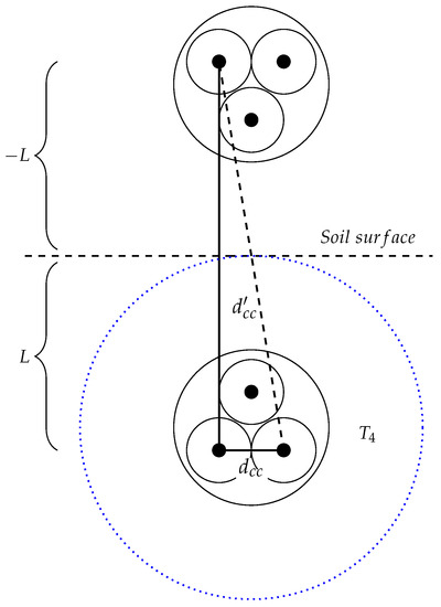
Figure 7.
Surrounding cable to soil surface dimensions and mirror of adjacent cable dimensions; representation of the surrounding thermal resistance (the drawing is not to scale).
- Metallic layers are neglected, as their thermal resistance is negligible compared with that of poly-composite materials.
- The optical fibre inside the fillers is assumed to have no thermal impact.
- Swelling tape is assumed to be a part of the insulation since its thickness is small, and it is assumed to have the same thermal resistivity.
- The bedding material is assumed to be the same material as that composing the anti-corrosion sheath.
Figure 8 shows a static thermal representation of a three-core cable based on the cable construction in Figure 2, where the electrical resistances are equivalent to the thermal resistances, as shown in Figure 5 and Figure 6, and define the ability of the materials to impede heat flow. In Figure 8, is the conductor temperature, is the outer covering (cable surface) temperature and is the ambient temperature of the surroundings. As the cable is a three-core cable, and represents the resistance of the inner cables, the circuit is represented with as three resistances in parallel.
Figure 8.
Static representation of thermal resistances in a three-core XLPE SL-type submarine cable, including power losses located in the respective layers and temperature denotation.
The thermal resistances shown in Figure 8 are determined by Equations (9)–(12) [11], where the thermal resistivity for commonly used cable materials and surrounding seabed conditions is defined in Table 1, t is the thickness of the respective cable layers, is the conductor diameter, is the outer diameter of the armour, is the outer cable diameter, is a geometric factor as a function of thickness of material between sheaths and armour and expressed as a fraction of the outer diameter of the sheath in Equation (13).

Table 1.
Commonly used thermal resistivity for materials and surroundings.
The geometric factor is found as the function and is determined by Equation (14) [11].
2.2.3. Static Temperature Calculation
IEC 60287-1-1 describes the calculation of current rating and losses at load. However, with the method proposed in this paper, more accurate results can be achieved. In the proposed method, it is assumed that the cable loading is known. IEC assumes a maximum conductor temperature of C; for the proposed method, this value is calculated by an iterative process with the steady-state reached temperature given by Equation (15) [10].
2.3. Thermal Cable Analysis of Transient Conditions
A three-core XLPE submarine cable contains multiple non-conductive layers. An equivalent electrical circuit can be developed to represent the thermal properties of the cable layers according to the thermal-electrical analogous parameters.
By constructing a thermal analogy ladder network, it is possible to study the thermal behaviour in the centre of the conductor. Equation (16) is used to calculate the thermal capacitance of the respective layers, where S is the cross-sectional area of the respective layer, and is the specific heat capacity of the material. Typical heat capacity values can be found in Table 1.
2.3.1. Thermal Ladder Network Construction
To analyse the transient temperature response in the centre of the conductor, it is essential to thermally model the cable with high accuracy. The cable is transformed from the three-core cable into a single-core equivalent cable with the same thermal properties to simplify the equivalent thermal circuit. According to IEC 60853-2 [8], transients greater than 1 h are assumed to be long duration transients, which usually is the case, of an offshore wind farm. Therefore, this method is based on long transients and is intended for the use of long duration temperature transients only. The ladder network method (LNM) is only applicable in cases where the thermal parameters do not change as a function of temperature variations, as it solves heat flow equations using the superposition principle, which is used exclusively for linear systems.
Figure 9 shows a quarter of the cross-section of the equivalent single-core cable, with thermal resistances represented on the x-axis below the respective layer and thermal capacitances represented on the left-hand side of the y-axis beside the respective layer.
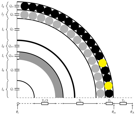
Figure 9.
Quarter cross-sectional area of a single-core XLPE SL-type equivalent submarine cable with thermal resistances T and thermal capacitances Q represented along the axes.
To visually demonstrate the modelling of the total thermal ladder network representing a three-core XLPE submarine cable, the ladder network is divided into three sections, each surrounding a thermal resistance.
Representing the insulation layer and the screens surrounding it, the thermal resistances are divided by three, , to represent the three internal parts of the cable in parallel. The thermal capacitance of the insulation is divided into two non-equal lumped parameters, distributed in parallel on each side of the thermal resistance . Figure 10 shows the thermal representation of the dielectric layers, where Van Wormer’s coefficient, shown in Equation (17), is applied to determine the allocation of the thermal capacitance more accurately [9].
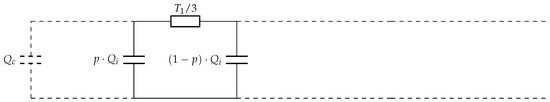
Figure 10.
Transient representation of thermal parameters for insulation.
In order to improve the accuracy in the use of lumped parameters, the thermal insulation capacitance is distributed between the single-core equivalent conductor diameter given in Equation (18) and the external diameter of insulation using Van Wormer’s coefficient p [9], shown in Equation (17), for long duration transients.
As mentioned before, due to the asymmetry of the internal parts of the three-core cable shown in Figure 8, the allocation of thermal resistance has to be defined as an equivalent single-core conductor diameter dissipating the same losses as that determined by Equation (18).
Representing the sheaths around the thermal resistance , the metallic sheath and anti-corrosion sheath are distributed on each side of , as they do not have the same specific heat capacity coefficient . Due to the asymmetry of the internal part of the cable, the thermal resistance is calculated using the geometric factor to include the fillers in the thermal resistance [10].
Estimations of the single-core diameter of the fillers are made on the basis of the assumption that each layer is occupied by insulation, and this means that the thermal capacitance is separated into two equal capacitances because the diameter varies in the original three-core cable. Figure 11 shows the distribution of the sheath parameters.
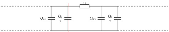
Figure 11.
Transient representation of thermal parameters for sheath.
To represent the cable’s outer covering surrounding the thermal resistance , the armour and the outer serving layer must be distributed around. As the armour is a metallic layer, the thermal capacitance is placed in the original position, and the thermal capacitance of the outer serving is divided into two capacitances by Van Wormer’s coefficient in Equation (19) to allocate the thermal capacitance distribution of the outer covering [8]. Figure 12 shows the distributed parameters of the armour and the outer covering.
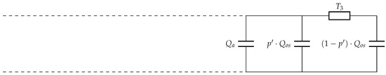
Figure 12.
Transient representation of thermal parameters for outer covering.
By developing lumped parameters for each part of the cable, a three-core XLPE submarine cable is thermally represented by connecting the models of Figure 10, Figure 11 and Figure 12, as shown in Figure 13.
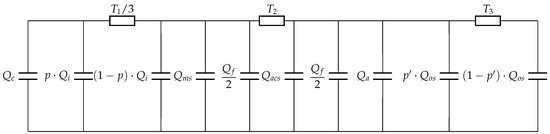
Figure 13.
Thermal three-core XLPE submarine cable ladder network.
To represent the cable in operation, the thermal ladder network must include the cable losses. Using the Cigre two-loop method [8] to reduce the mathematical complexity of the circuit analysis, the final thermal ladder network including power losses can be derived as shown in Figure 14, where is the denotation of the conductor temperature and represents the temperature at the outer serving.
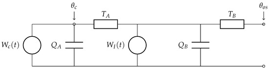
Figure 14.
Reduced thermal ladder network representing a three-core XLPE submarine cable.
According to IEC 60853-2 [8], the apparent thermal resistances in the ladder network can be defined as shown in Equations (20) and (21), and the apparent thermal capacitances are defined in Equations (22) and (23). The cable losses are equally found; cable conductor loss is determined by Equation (24), and the total internal cable losses , including dielectric, sheath and armour losses, are determined by Equation (25).
2.3.2. Transient Temperature Response to a Step Function
To evaluate the transient temperature behaviour in the centre of the conductor resulting from an applied step function, it is necessary to model the thermal temperature response mathematically. A step function is made to reduce the number of calculations needed. Figure 15 illustrates a current step function with a total number of i 4 h constant load steps . is the average value of the actual flowing current for each step during the current profile segment illustrated in Figure 3.
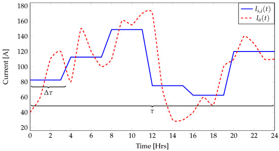
Figure 15.
Step function construction of a wind-based load profile.
To determine an appropriate length for the constant time-steps , an empirical calculation was proposed by George J. Anders [9] as given by Equation (26). This method was proposed at a time when computing time meant a lot; nowadays, the computing time is not an issue. Considering wind-based load profiles, it is not recommendable to use time-steps greater than 4 times the data resolution, as it does not represent the behaviour of the wind.
In this case, the step function has to represent the dynamic power losses, and , inside the cable, as shown in Figure 14 and determined by Equations (24) and (25).
Fourier transform of the unit impulse [9] as the transfer function is used to represent the response of the network [9]. The transfer function of the two-loop network shown in Figure 6 can be represented by the ratio between the conductor temperature and the cable power losses , according to Equation (27).
where and are polynomial of the transfer function obtained by Kirchhoff’s current law of the two-loop network; s is the complex transfer function variable. Considering any node h in the thermal ladder network, the temperature response as function of time can be expressed as shown in Equation (28) [8].
where is the time constant [s]; is a thermal coefficient [K · m/W]; t is time [s]; h is the node index; J is the loop index (1, 2); and are obtained from poles and zeros of the transfer function given in Equation (27).
The coefficient is given by Equation (29), developed by Valkenburg [8].
where is a coefficient of the numerator equation; is the first coefficient of the denominator equation; denotes zeros and poles of the transfer function, respectively; denotes poles. As the equivalent circuit shown in Figure 14 only consists of two loops (J = 1, 2) and the purpose of this analysis is to obtain the conductor temperature, represented in loop one (h = 1), from Equation (29) is simplified using the notation in the following Equations (30) and (31), where is the thermal coefficient of loop one, and is the thermal coefficient of loop two.
From Equation (27), zeros of the transfer function are obtained as shown in Equation (32), and the poles and representing each of the loops are obtained as shown in Equations (33) and (34) [8,9].
To simplify the notation of the poles, the substitutions shown in Equations (35) and (36) are applied [9].
From Equation (27), can be found as shown in Equation (37) for loop one, and is found in Equation (38). Thus, the first part of Equation (29) can be found as shown in Equation (39).
Multiplying from Equation (33) with from Equation (34), an expression is found in Equation (41) to reduce the thermal coefficients.
Using Equation (41) to simplify Equation (40), an expression is found and shown in Equation (42) to find the thermal coefficient of the first loop in the thermal ladder network. Following the same procedure for the thermal coefficient of the second loop, an expression is found and shown in Equation (43).
With the thermal coefficients determined for each of the loops in the thermal ladder network, the total transient temperature response above the ambient temperature is available. The total temperature transient is found as the function of three contributing transients that are due to the ith load step of the step functions and , as shown in Equation (44).
The transient temperature response , which is derived from Equation (28), describes the conductor () to cable surface () transient temperature response as a function of time in Equation (45).
IEC 60853-2 [8] proposes a method to determine the transient temperature rise and fall due to the impact of the surrounding conditions. The function is developed from an isotherm process between the centre of the conductor and the soil surface, as shown in Figure 7. The temperature response from the surroundings is given as an exponential integral function in Equation (46).
where is the exponential integral, defined as , which can be developed in the series shown in Equation (47); is the distance from the centre of the conductor to the image of an adjacent conductor centre [m]. Figure 7 shows the relation between the burial depth L and the conductor centre to centre distance and an approximation to determine the distance from the centre of the conductor to the image of an adjacent conductor centre, given by Equation (48).
To determine the real temperature gradient of the first part of a temperature response from the surroundings, an attainment factor is added. The attainment factor is computed as the ratio of the first part of the transient to the same segment in steady-state. This factor takes into account the heat dissipation from the centre of the conductor to the cable surface and is calculated by Equation (49) [9].
With all three contributing transients from Equation (44) determined, it is possible to illustrate each of the transients and the total transient temperature response by an example, shown in Figure 16. In this figure, each contributing transient due to one current step i (i = 1) is evaluated for a step time duration of 24 [h]. The figure shows that the conductor to cable surface temperature rises due to one step of the dynamic power loss function . As expected, the temperature rises rapidly during the first part of the transient, after which it exponentially reaches the steady-state temperature after a certain period. At this time, a common temperature of the cable for the layers between the conductor and the cable surface is achieved. The attainment factor is intended to describe the ratio of the first part of the transient to the same segment in steady-state. It is multiplied by the temperature response of the surrounding conditions and is intended to attain the real ability of the environment to absorb heat in the first part of the transient. The transient temperature response itself that results from the impact of the surrounding conditions is modelled to determine the ability of the environment to absorb heat as a function of time due to the total dynamic power loss function . Compared with the cable to surface transient , it is a long-term process to reach steady-state conditions, and it can be justified by the fact that the surroundings of the cable can be considered as a circular large thermal capacitance around the cable, as shown in Figure 7. Generally, in the first part of the temperature transient, the conductor to cable surface transient has a significant influence on the temperature increase. After a certain amount of time, it reaches a steady-state temperature, whereas the temperature response of the surrounding conditions still increases.
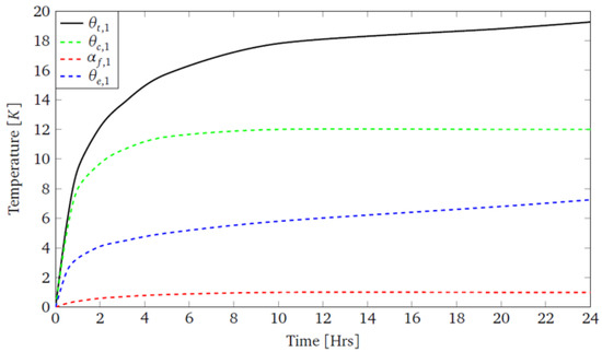
Figure 16.
Total transient temperature response of a single load step given by Equation (50).
By introducing multiple load steps, the superposition principle can be utilised as illustrated by Equation (50) to calculate the transient temperature as a function of time. Figure 17 shows three randomly selected load steps and the total temperature progress .
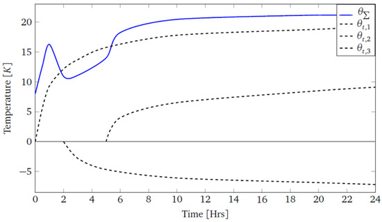
Figure 17.
Total transient temperature response of multiple load steps given by Equation (51).
Each evaluated temperature transient is calculated using multiple loops and is saved in a matrix. In order to sum the partial transients above an ambient temperature, an -matrix storing all partial temperature transients is formed, as shown in Equation (51).
The sum of all partial transient temperatures above ambient is determined as the temperature series of the sum of every single column in the matrix . To determine the complete temperature response to a forcing step function, the ambient temperature is added to the temperature series , as shown in Equation (52).
3. Results
This study shows how to construct a thermal ladder network that represents three-core XLPE submarine cables at 36 kV AC and above. By deriving the thermal coefficient contained in the thermal ladder network from the Fourier transfer function, it is possible to describe the temperature behaviour in the centre of the cable by applying a load step to the cables. Using the superposition principle, this study proves the ability to represent a load profile by the sum of each temperature transient.
The study could be extended to a cable ageing analysis, as the most noticeable wear on cables is due to temperature changes, using an insulation ageing diagnosis of XLPE power cables. These parameters are a significant part of the developed calculations and can potentially be extended to analyse the lifetime of the cables on the basis of an estimated load profile [17].
4. COMSOL Multiphysics Finite Element Method (FEM) Validation
To compare the results of the temperature evaluation performed on the basis of the thermal LNM calculations with simulations performed by an FEM, the cable construction, materials and surrounding conditions must be identical. The FEM is a computer-based calculation method solving partial differential and integral equations. It is based on a unique connection between the field sizes in nodes and field sizes anywhere in the element and solved as a mathematical interpolation problem. The purpose of this validation is to analyse the transient temperature behaviour in the centre of the cable and compare the results between the two methods.
No-Load Full-Load Test of a 220 kV 3× 1800 [] XLPE SL Type Submarine Cable
In this subsection, a validation of the proposed method is presented with an estimated 220 kV 3×1800 [mm] Al XLPE submarine cable. The validation was performed using the cable data shown in Table A1 and surrounding conditions in Table A2 in Appendix A. The test is a full-load no-load test, where the cable is applied to two long-term step sequences. This test aims to show the entire transient temperature progress due to a step applied to the cable until it nearly reaches steady-state temperature conditions. The first step is a 2000 [h] step with a current loading of 930 [A] corresponding to 100% load, and the second step is similar: a 2000 [h] step with a current loading of 0 [A] corresponding to 0% load, as shown in Appendix A, Figure A1. The test result is illustrated in Figure 18 and shows major agreement between the two methods used to evaluate the transient temperature behaviour in the same cable. The FEM-based approach is represented by the blue line and the LNM-based method is represented with orange. Comparing the transient temperature behaviours caused by the full-load and the no-load step shows almost identical temperature behaviours.
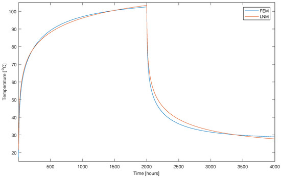
Figure 18.
Transient temperature response to a full-load no-load current step for COMSOL Multiphysics finite element method (FEM) validation of a 220 [kV] 3×1800 [mm] Al XLPE SL-type submarine cable.
The temperature progress of the FEM-based and LNM-based evaluation shows that the transient temperature curves cross each other twice on each step. The first part of the transient is almost identical until they cross the first time, after which temperature differences occur. From Figure 16, it can be concluded that the deviation at the end of the temperature progression is caused by the modelling of the surroundings.
The difference in the calculation methods causes the deviation. The transient temperature evaluation using the FEM is divided into an infinite number of small thermal capacitances that are continuously charged along the layer of the cable. Using the LNM, the thermal capacitances are modelled as two dominant thermal capacitances and . The maximum negative temperature deviation in this test is 1.19 [C].
5. Discussion
On the basis of this study, there are several topics to discuss and, furthermore, to highlight as potential future study areas and applications for use. In comparison with previous works with similar hypotheses, the proposed proved to be a very efficient approach to performing thermal temperature analysis. Previous works on cables or overhead lines have been conducted to improve the current ampacity of existing lines and often used a DTS system for emergency rating. The method presented in this article is a simple process to evaluate the temperature progress with acceptable deviations compared to an FEM-based simulation. The point where this method is preferable is that, instead of a simulation time measured in a couple of hours, this method can determine a dynamical rating in just a few minutes. Therefore, this method can be used together with the FEM to reduce the number of simulations for an initial cable guess, since the LNM provides a good starting point for the cable rating phase. As pointed out in the study, some of the approaches from the approved standards can be considered questionable. In particular, the calculation of armour losses has been found to be significantly higher using IEC’s method. Using a two-loop reduction method of the thermal ladder network creates some deviations. The deviation is caused by the difference in the calculation method, as the transient temperature evaluation using the FEM is divided into an infinite number of small thermal capacities that are continuously charged along the thickness of the layer inside the cable. Using the LNM, the thermal capacitances are modelled as two dominant thermal capacitances, and . This method is directly able to take a quick first shot at a dynamic rating of a three-core XLPE submarine cable. In addition, it will be possible to use a method like this to check the cable supplier’s calculations. Looking at the proposed method in a broader context, it would be available for making continuous temperature estimations on the basis of a loading forecast and the use of a DTS system to measure the reference temperature. In this case, users should be aware of the limitation of the individual time constant of the cables found in Equation (53) [8].
6. Materials and Methods
To perform this study, 17 different references were used. There are four sources that establish the foundation for recreating the calculations and results obtained through this study. The first three sources are all approved standards written by IEC—IEC 60287-1-1: 2006; IEC 60287-2-1: 2015; IEC 60853-2: 1989. The last source is by George J. Anders, “Rating of Electric Power Cables— Ampacity Computations for Transmission, Distribution and Industrial Applications”: 1997. It provides extended explanations and derivations of terms described in the IEC standards.
7. Conclusions
This article shows how to determine internal cable parameters and model the thermal ladder network to represent a three-core XLPE submarine cable with heat dissipation from the surroundings. It proposes an iterative method combining two approved standards to make a dynamic rating of three-core XLPE submarine cables by an evaluation of the transient temperature behaviour in the centre of the conductor. The method is validated in comparison with an FEM-based simulation and shows, in the above specific case, a maximum deviation of 1.19 C. In comparison with an FEM-based approach, the method presented in this article is remarkably faster at evaluating the temperature progress and will, in most cases, be a good first-shot computation of the cable rating phase of a project.
Author Contributions
T.V.M.N. and S.J. developed methodology, performed the analysis, modelling and software simulation study, write the draft manuscript and the revised version. M.S. supervised the research activities: In addition, he reviewed and commented on the original and revised manuscripts.
Acknowledgments
This study was made as a part of the education Electrical Power Engineering at the 7th semester, at the University of Southern Denmark, Odense, Denmark. Thanks to the cooperating companies Energinet Eltransmission A/S and Vattenfall Wind Power A/S for the contribution of the needed data and expert knowledge, when needed.
Conflicts of Interest
The authors declare no conflict of interest.
Abbreviations
The following abbreviations are used in this manuscript:
| AC | Alternating Current |
| Al | Aluminium |
| CIGRE | Conseil International des Grands Réseaux Électriques (International Council on Large Electric Systems) |
| Cu | Copper |
| DC | Direct Current |
| DLR | Dynamic Line Rating |
| DTS | Distributed Temperature Sensing |
| FEM | Finite Element Method |
| HVAC | High Voltage Alternating Current |
| IEC | International Electrotechnical Commission |
| LEC | Levelised Energy Costs |
| LNM | Ladder Network Method |
| MDPI | Multidisciplinary Digital Publishing Institute |
| SL | Separate Lead Sheath |
| WTG | Wind Turbine Generator |
| XLPE | Cross-linked Polyethylene |
Appendix A. Cable Data, Surrounding Conditions and Step Function for COMSOL Multiphysics Finite Element Method Validation
Table A1.
Cable data for COMSOL Multiphysics FEM validation of an estimated 220 [kV] 3×1800 [mm] Al XLPE SL-type submarine cable (cable layer numbering according to Figure 2).
Table A1.
Cable data for COMSOL Multiphysics FEM validation of an estimated 220 [kV] 3×1800 [mm] Al XLPE SL-type submarine cable (cable layer numbering according to Figure 2).
| Layer | Thickness t [mm] | Material |
|---|---|---|
| 25.9 | Al | |
| 1.70 | XLPE | |
| 23.0 | XLPE | |
| 1.70 | XLPE | |
| 0.60 | PE | |
| 3.10 | LA | |
| 2.50 | PE | |
| 3.00 | PE | |
| 5.00 | St | |
| 4.00 | PP |
Table A2.
Surrounding conditions for COMSOL Multiphysics FEM validation of an estimated 220 [kV] 3×1800 [mm] Al XLPE SL-type submarine cable.
Table A2.
Surrounding conditions for COMSOL Multiphysics FEM validation of an estimated 220 [kV] 3×1800 [mm] Al XLPE SL-type submarine cable.
| Parameter | Unit | Value |
|---|---|---|
| Burial depth L | [m] | 10.0 |
| Ambient temperature | [C] | 15.0 |
| Thermal soil resistivity | [K·m/W] | 0.9 |
| Soil diffusivity | [m/s] |

Figure A1.
Full-load no-load current step for COMSOL Multiphysics FEM validation of a 220 [kV] 3×1800 [mm] Al XLPE SL-type submarine cable.
References
- European Commission. 2030 Climate & Energy Framework. Available online: https://ec.europa.eu/clima/policies/strategies/2030 (accessed on 6 November 2018).
- Dupin, R.; Michiorri, A. Renewable Energy Forecasting: From Models to Applications, 1st ed.; Kariniotakis, G., Ed.; Woodhead Publishing: Sawston, UK; Cambridge, UK, 2017; p. 325. [Google Scholar]
- Hemparuva, R.J.C.; Simon, S.P.; Kinattingal, S.; Padhy, N.P. Geographic information system and weather based dynamic line rating for generation scheduling. Eng. Sci. Technol. Int. J. 2018, 21, 564–573. [Google Scholar] [CrossRef]
- GWEC. Global Statistics. Available online: http://gwec.net/global-figures/graphs (accessed on 8 November 2018).
- Ebenhoch, R.; Matha, D.; Marathe, S.; Muñoz, P.C.; Molins, C. Comparative Levelized Cost of Energy Analysis. Energy Procedia 2015, 80, 108–122. [Google Scholar] [CrossRef]
- Huang, R.; Pilgrim, J.A.; Lewin, P.L.; Payne, D. Dynamic cable ratings for smarter grids. In Proceedings of the IEEE PES ISGT Europe 2013, Lyngby, Denmark, 6–9 October 2013. [Google Scholar]
- Li, H.; Tan, K.; Su, Q. Assessment of underground cable ratings based on distributed temperature sensing. IEEE Trans. Power Deliv. 2006, 21, 1763–1769. [Google Scholar] [CrossRef]
- International Electrotechnical Commision. IEC 60853-3:1989 Calculation of the Cyclic and Emergency Current Rating of Cables. Part 2: Cyclic Rating of Cables Greater Than 18/30 (36) kV and Emergency Ratings for Cables of All Voltages; International Electrotechnical Commission: Geneva, Switzerland, 1989. [Google Scholar]
- Anders, G.J. Rating of Electric Power Cables: Ampacity Computations for Transmission, Distribution, and Industrial Applications; IEEE Press: New York, NY, USA, 1997. [Google Scholar]
- International Electrotechnical Commision. IEC 60287-1-1:2006 Electric Cables—Calculation of the Current Rating—Part 1-1: Current Rating Equations (100 % Load Factor) and Calculation of Losses—General; International Electrotechnical Commission: Geneva, Switzerland, 2006. [Google Scholar]
- International Electrotechnical Commision. IEC 60287-2-1:2015 Electric Cables—Calculation of the Current Rating—Part 2-1: Thermal Resistance—Calculation of the Thermal Resistance; International Electrotechnical Commission: Geneva, Switzerland, 2015. [Google Scholar]
- Palmgren, D.L. Armour Loss in Three-Core Submarine XLPE Cables; ABB AB: Växjö, Sweden, 2013. [Google Scholar]
- Goddard, K.F.; Pilgrim, J.A.; Chippendale, R.; Lewin, P.L. Induced losses in three-core SL-type high-voltagecables. IEEE Trans. Power Deliv. 2015, 30, 1505–1513. [Google Scholar] [CrossRef]
- Brakelmann, H.; Stammen, J. Thermal Emissions of the Submarine Cable Installation Viking Link in the German AWZ; BCC Cable Consulting: Rheinberg, Germany, 2017. [Google Scholar]
- Aegerter, D.; Meier, S. Cableizer—Parameter. 2018. Available online: https://www.cableizer.com/documentation/sigma1/ (accessed on 22 October 2018).
- Engineeringtoolbox. Specific Heats for Metals. 2003. Available online: https://www.engineeringtoolbox.com/specific-heat-metals-d152.html (accessed on 5 November 2018).
- Liu, F.; Huang, X.; Wang, J.; Jiang, P. Insulation ageing diagnosis of XLPE power cables under service conditions. In Proceedings of the 2012 IEEE International Conference on Condition Monitoring and Diagnosis, Bali, Indonesia, 23–27 September 2012. [Google Scholar]
© 2019 by the authors. Licensee MDPI, Basel, Switzerland. This article is an open access article distributed under the terms and conditions of the Creative Commons Attribution (CC BY) license (http://creativecommons.org/licenses/by/4.0/).