Numerical Evaluation of Sample Gathering Solutions for Mobile Robots

Abstract

This paper applies mathematical modeling and solution numerical evaluation to the problem of collecting a set of samples scattered throughout a graph environment and transporting them to a storage facility. A team of identical robots is available, where each robot has a limited amount of energy and it can carry one sample at a time. The graph weights are related to energy and time consumed for moving between adjacent nodes, and thus, the task is transformed to a specific optimal assignment problem. The design of the mathematical model starts from a mixed-integer linear programming problem whose solution yields an optimal movement plan that minimizes the total time for gathering all samples. For reducing the computational complexity of the optimal solution, we develop two sub-optimal relaxations and then we quantitatively compare all the approaches based on extensive numerical simulations. The numerical evaluation yields a decision diagram that can help a user to choose the appropriate method for a given problem instance.

1. Introduction

Much robotics research develops automatic planning procedures for autonomous agents such that a given mission is accomplished under an optimality criterion. The missions are usually related to standard problems such as navigation, coverage, localization, and mapping [1,2]. Some works provide strategies directly implementable on particular robots with complicated dynamics and multiple sensors [3]. Other research aims to increase the task expressiveness [4], e.g., starting from Boolean-inspired specifications [5,6] up to temporal logic ones [7,8,9,10], even if the obtained plans may be applied only to simple robots.

It is often common to construct discrete models for the environment and robot movement capabilities, by using results from multiple areas such as systems theory, computational geometry [11,12], and discrete event systems [13,14].

The current research is focused on solving a sample gathering problem. The considered task belongs to the general class of optimal assignment problems [15], since the sample can correspond to jobs and the robots to machines. The minimization of the overall time for gathering all samples (yielded by the “slowest” agent) thus translates to so-called min-max problems [16] or bottleneck assignment problems [15] (Chapter 6.2). However, these standard frameworks do not consider different numbers of jobs and machines, nor machines (agents) with limited energy amounts.

A broad taxonomy of allocations in multi-robot teams is presented in [17,18], according to which our problem belongs to the class of assignments of single-robot tasks (one task requiring one robot) in multi-task robot systems (a robot can move, pick up, and deposit samples). Again, the general solutions assume utility estimates for different job–machine pairs.

For such problems, various Mixed-Integer Linear Programming Problem (MILP) formulations are given as in [17,19,20]. Some resemble our problem, but they are not an exact fit because of the specificities that all samples should be eventually gathered into the same node, a robot can carry one sample at a time, there are limited amounts of energy, and we do not know a priori a relationship between number of samples and number of robots. Furthermore, we provide a second MILP for the case of problems infeasible due to energy requirements. We further relax the complex MILP solutions into sub-optimal solutions as non-convex Quadratic Programming (QP) and iterative heuristics. Our goal is to draw rules of choosing the appropriate method for a given problem, based on extensive tests.

Some preliminary mathematical formulations that generalize traveling salesman problems are included in [21], with targeted application to exploring robots that must collect and analyze multiple heterogeneous samples from a planetary surface. Other works focus on specific applications as task allocation accomplished by agents with different dynamics [22], or allocation in scenarios with heterogenous robots that can perform different tasks [23]. Various works propose auction-based mechanisms for various assignments problems or develop and apply distributed algorithms for specific cases with equal number of agents and tasks [24]. Research [25] assumes precedence constraints on available tasks and builds solutions based on integer programming forms and auction mechanisms. However, we do not include auction-based methods here. The closest solution we propose may be our iterative heuristic algorithm from Section 4.2, which can be viewed as a specific greedy allocation method [17].

Our problem can be seen as a particular case of Capacity and Distance constrained Vehicle Routing Problem (CDVRP) [26] with capacity equal to one and the distance constrains related to the limited energy. For this problem, many algorithms have been provided, for the exact methods [27,28] and for heuristic methods [29,30,31,32]. However, our problem is different in multiple aspects. First, in the CDVRP problem, the capacity of each vehicle (robot in our case) should be greater than the demand of each vertex [26]. In our case this cannot hold since the robot capacity is one (we assume that each robot can transport maximum one good) and the number of goods at the vertices is, in many cases, greater than one. Second, up to our knowledge, the heuristics considered in this work, which include relaxing the optimal solution of the MILP to a QP problem, have not been considered for the CDVRP. Finally, most of the works on CDVRP try to characterize worst-case scenarios through cost differences between heuristic and optimal methods.

In this paper, we are also interested in the computational complexity and we evaluate the proposed solutions using numerical simulations. To the best of our knowledge, none of the mentioned works contains a directly applicable formulation that yields a solution for our specific problem. This work builds on solutions reported in [33,34,35]. In [33] we constructed a MILP problem that solves the minimum time sample gathering problem. Different than in [33], we also design a MILP solution that can be used when the initial problem is infeasible due to scarce energy limits. Besides the MILP formulations, one of the main goals of this research are to provide computationally efficient sub-optimal solutions for the targeted problems. The MILP solution was relaxed to a QP formulation in [34]. Here we also construct an iterative sub-optimal solution inspired by [35] as a QP alternative. Based on extensive simulations that involve the three proposed solutions, we conclude with a decision scheme that helps a user to choose the appropriate method for a specific problem instance.

The purpose of this work is to plan a team of mobile agents such that they gather the samples scattered throughout the environment into a storage facility. The problem’s hypothesis consists in a team of mobile robots which must bring to a deposit region a set of samples that exist in an environment at known locations. As main contributions we claim the new mathematical models for the considered problems and the numerical evaluation of the obtained solutions.

The environment is modeled by a graph where an arc weight corresponds to consumed energy and time for moving between the linked nodes. Each robot has limited energy, and the goal is to collect all samples in minimum time. Because the robots are initially deployed in the storage (deposit) node and given the static nature of the environment, it is customary to build movement plans before the agents start to move. The problem reduces to a specific case of optimal assignment or task allocation [15,17,18]. The paper combines results from our previous research reported in [34,36,37]. We first build an optimal solution involving a MILP formulation. Then, we design two solutions with lower complexities, one as a Quadratic Programming (QP) relaxation of the initial MILP, and the other as an Iterative Heuristic (IH) algorithm. A numerical evaluation between the formulated solutions yields criteria as time complexities for computing robotic plans and the difference of costs between these plans. Based on these criteria, a decision diagram is provided such that a user can easily choose the appropriate method to embed.

The remainder of the paper is structured as follows. Section 2 formulates the targeted problem, outlines the involved assumptions and introduces an example that will be solved throughout the subsequent sections. Section 3 details two optimal solutions, from which the first will be relaxed to a QP formulation, while the second can be used when robots have low energy supplies. The sub-optimal methods based on QP optimization or IH algorithm are presented in Section 4. The developed methods are numerically evaluated and compared in Section 5 and rules are given for choosing the proper method for a specific problem instance.

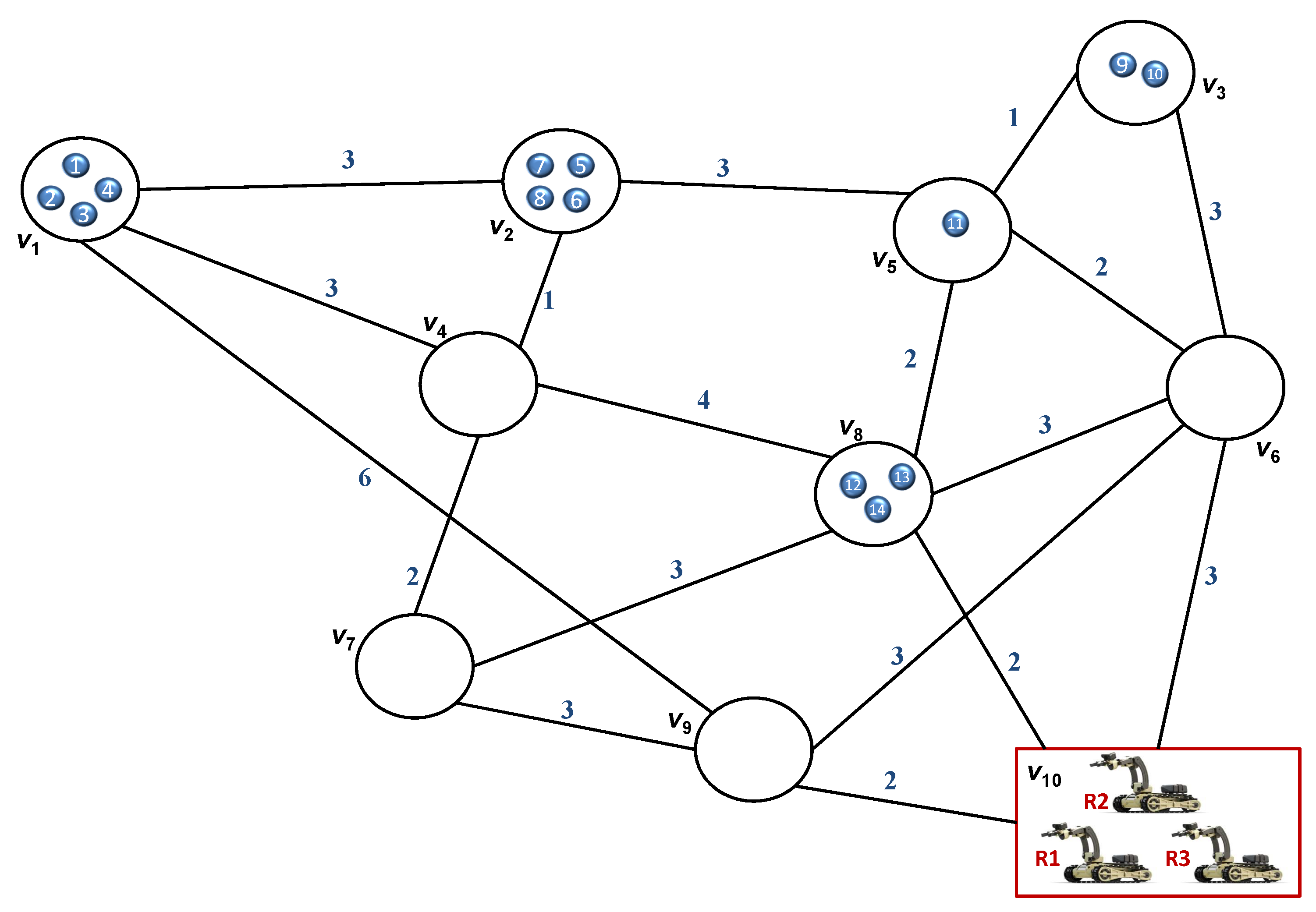
2. Problem Formulation

Consider a team of $N_R$ identical robots that are labeled with elements of set $R=\{r_1,r_2,\dots ,r_{N_R}\}$. The robots “move” on a weighted graph $G=(V,E,c)$, where $V=\{v_1,v_2,\dots ,v_{\left|V\right|}\}$ is the finite number of nodes (also called locations or vertices), $E\subseteq V\times V$ is the adjacency relationship corresponding to graph edges, and $c:E\to {\mathbb{R}}_{+}$ is a cost (weight) function.

We mention that there are multiple approaches for creating such finite-state abstractions of robot control capabilities in a given environment [1,2]. A widely used idea is to partition the free space into a set of regions via cell decomposition methods, each of these regions corresponding to a node from V [6,11,38]. The graph edges correspond to possible robot movements between adjacent partition regions, i.e., $\forall v,v^{\prime }\in V$, if an agent can move from location v to $v^{\prime }$ without visiting any other node from graph, then $(v,v^{\prime })\in E$. Each edge corresponds to a continuous feedback control law for the robot such that the desired movement is produced, and various methods exist for designing such control laws based on agent dynamics and partition types [39,40]. Alternatives to cell decomposition methods, as visibility graphs or generalized Voronoi diagrams, can also produce discrete abstractions in form of graphs or transition systems [1].

We assume that the graph G is connected, and the adjacency relationship E is symmetric, i.e., if a robot from R can travel from location v to $v^{\prime }$, then it can also move from $v^{\prime }$ to v. For any $(v,v^{\prime })\in E$, we consider that the cost $c(v,v^{\prime })$ represents the amount of energy spent by the robot for performing the movement from v to $v^{\prime }$ and that $c(v^{\prime },v)=c(v,v^{\prime })$. By assuming identical agents with constant velocity and a homogenous environment (i.e., the energy for following an arc is proportional with the distance between linked nodes), we denote the time necessary for performing the movement from location v to $v^{\prime }$ by $\gamma ·c(v,v^{\prime })$, where $\gamma \in {\mathbb{R}}_{+}$ is a fixed value.

Initially, all agents are deployed in a storage (deposit) node $v_{\left|V\right|}$ (labeled for simplicity as the last node in graph G), and each robot $r\in R$ has a limited amount of energy, given by map $\mathcal{E}:R\to {\mathbb{R}}_{+}$, for performing movements on abstraction G. For homogenous environments and constant moving speeds, energy $\mathcal{E}\left(r\right)$ can be easily linked with battery level of robot r, with the distance it can travel, or the sum of costs of followed edges.

There are $N_S$ samples or valuable items scattered throughout the environment graph G. The samples are indexed (labeled) with elements of set $S=\{1,2,\dots ,N_S\}$, while a map $\pi :S\to V$ shows to which node each sample belongs.

Problem 1.

For every robot $r\in R$ find a moving strategy on G such that:

• the team of robots gathers (collects) all samples from graph G in the storage node $v_{\left|V\right|}$ within minimum time;
• each robot can carry at most one sample at any moment;
• the total amount of energy spent by each robot is at most its initially available energy.

Remark 1

(NP-hardness). Our problem is related to the so-called Set Partitioning Problems (SPPs) [17], which are employed in various task allocation problems for mobile agents. A SPP formulation aims to find a partition of a given set such that a utility function defined over the set of acceptable partitions with real values is maximized. Various SPPs are solved by using Operations Research formulations that employ different standard optimization problems. In our case, the given set is S (samples to be collected), while the desired partition should have $N_R$ disjoint subsets of S, each subset corresponding to the samples a robot should collect. The utility relates to the necessary time required for collecting all samples (being a maximum value over utilities of elements of obtained partition), while the partition is acceptable if each robot has enough energy to collects its samples. The maximization over individual utilities show that our problem is more complicated than standard SPPs. Since an SPP is NP-hard [41], we conclude that Problem 1 is also NP-hard. Therefore, we expect computationally intensive solutions for optimally solving Problem 1, while sub-optimal relaxations may be used when an optimal solution does not seem tractable.

Since the sample deployment and robot energy limits are known, the searched solution is basically an off-line computed plan (sequence of nodes) for each robot such that the mission requirements are fulfilled. The first requirement from Problem 1 can be regarded as a global target for the whole team (properly assign robots to collect samples such that the overall time for accomplishing the task is minimized), while the last two requirements are related to robot capabilities. As in many robot planning approaches where global tasks are accomplished, we do not account for inter-robot collisions when developing movement plans. In real applications, such collisions can be avoided by using local rules during the actual movement, and the time (or energy) offset induced by such rules is negligible with respect to the total movement time (or required energy). Clearly, in some cases Problem 1 may not have a solution due to insufficient available energy for robots, these situations will be discussed during solution description.

Example 1.

For supporting the problem formulation and solution development, we introduce an example that will be discussed throughout the next sections. Thus, we assume an environment abstracted to the graph from Figure 1, composed by 10 nodes ($v_1,v_2,\dots ,v_{10}$), with the deposit $v_{10}$. The costs for moving between adjacent nodes are marked on the arcs from Figure 1, e.g., $c(v_{10},v_8)=2$. The team consists of 3 robots labeled with elements of set $R=\{r_1,r_2,r_3\}$. For simplicity of exposition, we consider $\gamma =1$ (the constant that links the moving energy with necessary time) and equal amounts of energy for robots, $\mathcal{E}\left(r\right)=100$, $\forall r\in R$. There are 14 samples scattered in this graph (labeled with numbers from 1 to 14), with locations given by map π, e.g., $\pi \left(9\right)=\pi \left(10\right)=v_3$.

The problem requires a sequence of movements for each robot such that all the 14 samples are gathered into storage $v_{10}$, each robot being able to carry one sample at any time.

3. Mathematical Model and Optimal Solution

To solve Problem 1, defined in the previous section, our approach consists from the following main steps:

(i)

Determine optimal paths in graph G from storage node to all nodes containing samples.

(ii)

Formulate linear constraints for correctly picking samples and for not exceeding robot’s available energy based on a given allocation of each robot to pick specific samples.

(iii)

Create a cost function based on robot-to-sample allocation and on necessary time for gathering all samples.

(iv)

Cast the above steps in a form suitable for applying existing optimization algorithms and thus find the desired robot-to-sample allocations.

Step (i) is accomplished by running a Dijkstra algorithm [42] on the weighted graph G, with source node $v_{\left|V\right|}$ and with multiple destination nodes: $v\in V$ for which $\exists s\in S$ such that $\pi \left(s\right)=v$. Please note that a single run of Dijkstra algorithm returns minimum cost paths to multiple destinations.

Let us denote with $path\left(v\right)$ the obtained path (sequence of nodes) from deposit $v_{\left|V\right|}$ to node $v\in V$ and with $\omega \left(v\right)/2$ its cost. Due to symmetrical adjacency relationship of G, the retour path from v to storage is immediately constructed by following $path\left(v\right)$ in inverse order. The retour path is denoted by $pat{h}^{-1}\left(v\right)$ and it has the same cost $\omega \left(v\right)/2$. (Because are interested in the round-trip cost between nodes $v_{\left|V\right|}$ and v, we denote the one-way cost by $\omega \left(v\right)/2$ and thus the cost of the full path is simply denoted by $\omega \left(v\right)$.). Therefore, for collecting and bringing to storage location the sample $s\in S$, a robot spends $\omega \left(\pi \left(s\right)\right)$ for the round-trip given by $path\left(\pi \left(s\right)\right)$, $pat{h}^{-1}\left(\pi \left(s\right)\right)$.

For solving steps (ii)–(iv), let us first define a decision function as $x:N_R\times N_S\to \{0,1\}$ by:

$$x(r,s)=\left\{\begin{array}{cc}1,\hfill & \mathrm{if}\mathrm{robot}r\mathrm{picks}\mathrm{sample}s\hfill \\ 0,\hfill & \mathrm{otherwise}\hfill \end{array}\right.,\forall r\in R,s\in S.$$

(1)

The actual values returned by map x for any pair $(r,s)\in R\times S$ give the most important part of solution to Problem 1, and these values are unknown, yet. The outcomes of x will constitute the decision variables in an optimization problem that is described next.

Step (ii) is formulated as the following set of linear constraints:

$$\begin{array}{cc}{\displaystyle {\displaystyle \sum _{r\in R}}}x(r,s)=1,\hfill & \hfill \forall s\in S\\ {\displaystyle {\displaystyle \sum _{s\in S}}}\left(\omega \left(\pi \left(s\right)\right)·x(r,s)\right)\le \mathcal{E}\left(r\right),\hfill & \hfill \forall r\in R\end{array},$$

(2)

where the first set of equalities impose that exactly one robot is sent to collect each sample, while the subsequent inequalities guarantee that the energy spent by robot r for collecting all its assigned samples does not exceed its available energy.

The cost function from step (iii) corresponds to the first requirement of Problem 1. It means to minimize the maximum time among all robots required for collecting the assigned samples, and it formally translates to finding outcomes of x that minimize the objective function $J\left(x\right)$ from

$$J\left(x\right)={\displaystyle \underset{x}{min}}{\displaystyle \underset{r\in R}{max}}\left(\gamma ·{\displaystyle \sum _{s\in S}}\left(\omega \left(\pi \left(s\right)\right)·x(r,s)\right)\right).$$

(3)

The objective function from (3) and the constraints from (2) form a minimax optimization problem [43,44]. However, decision function x should take binary values. To use available software tools when solving for values of x, step (iv) transforms the minimax optimization into a MILP problem [44,45], by adding an auxiliary variable $z\in {\mathbb{R}}_{+}$ and additional constraints that replace the max term from (3). This results in the following MILP optimization:

$$\begin{array}{cc}{\displaystyle \underset{x,z}{min}}\hfill & z\hfill \\ \mathrm{s}.\mathrm{t}.:\hfill & {\displaystyle \sum _{r\in R}}x(r,s)=1,\forall s\in S\hfill \\ & {\displaystyle \sum _{s\in S}}\left(\omega \left(\pi \left(s\right)\right)·x(r,s)\right)\le \mathcal{E}\left(r\right),\forall r\in R\hfill \\ & \gamma ·{\displaystyle \sum _{s\in S}}\left(\omega \left(\pi \left(s\right)\right)·x(r,s)\right)\le z,\forall r\in R\hfill \\ & x(r,s)\in \{0,1\},\forall (r,s)\in R\times S\hfill \\ & z\ge 0\hfill \end{array}.$$

(4)

The MILP (4) can be solved by using existing software tools [46,47,48]. The solution is guaranteed to be globally optimal because both the feasible set defined by the linear constraints from (4) and the objective function (z) are convex [45,49]. Thus, solution of (4) gives the optimal outcomes for x (unknown decision variables $x(r,s)$), as well as the time z in which the team solves Problem 1.

Please note that the obtained map x indicates the samples that must be collected by each robot, as in (1). However, it does not impose any order for collecting these samples. For imposing a specific sequencing, each robot is planned to collect its allocated samples in the ascending order of the necessary costs. This means that robot r first picks the sample s for which $x(r,s)=1$ and $\omega \left(\pi \left(s\right)\right)\le \omega \left(\pi \left(s^{\prime }\right)\right)$, $\forall s^{\prime }\in S$ with $x(r,s^{\prime })=1$, and so on for the other samples. The optimum path for collecting sample s from node $\pi \left(s\right)$ was already determined in step (i). Under the above explanations, Algorithm 1 includes the steps for obtaining an optimal solution for Problem 1.

Algorithm 1: Optimal solution

Input: $G,R,S,\mathcal{E},\pi$    Output: Robot movement plans

Example 2.

We apply the optimal solution from this section on the example introduced in Section 2. The Dijkstra algorithm (line 1 from Algorithm 1) returns paths and corresponding energy for collecting each sample, e.g., $path\left(\pi \left(1\right)\right)=path\left(v_1\right)=v_{10},v_9,v_1$ and $\omega \left(\pi \left(1\right)\right)=16$. The MILP (4) was solved in about 0.7 s and it returned an optimal solution with $z=54$ (time for fulfilling Problem 1) and allocation map x. Based on robot-to-sample allocations x, lines 3–13 from Algorithm 1 yield the robotic plans for collecting samples from the following nodes (the sequences of nodes and the collect/deposit commands are omitted due to their length):

$$\begin{array}{c}Robot{r}_{1}collectssamplesfrom:\hfill \\ \left(v_8\right),\left(v_8\right),\left(v_2\right),\left(v_1\right),\left(v_1\right)\hfill & \hfill (\mathrm{time}:54)\\ Robot{r}_{2}collectssamplesfrom:\hfill \\ \left(v_3\right),\left(v_2\right),\left(v_2\right),\left(v_1\right)\hfill & \hfill (\mathrm{time}:54)\\ Robot{r}_{3}collectssamplesfrom:\hfill \\ \left(v_8\right),\left(v_5\right),\left(v_3\right),\left(v_2\right),\left(v_1\right)\hfill & \hfill (\mathrm{time}:52)\end{array}$$

(5)

In the remainder of this section we focus on the situation in which the mobile robots cannot accomplish Problem 1 due to energy constraints.

Remark 2.

Relaxing infeasible problems:If MILP (4) is infeasible, this means that Problem 1 cannot be solved due to insufficient available energy of robots for collecting all samples.

Intuitive argument. Whenever (4) has a non-empty feasible set (the set defined by the linear constraints), it returns an optimal solution from this set [45,49]. The feasible set can become empty only when the first two sets of constraints and the fourth ones from (4) are too stringent. The third set of constraints cannot imply the emptiness of feasible set, because there is no upper bound on z. It results that (4) has no solution whenever the first, second and fourth sets of its constraints cannot simultaneously hold. The fourth constraints cannot be relaxed, and therefore only the first two sets may imply the infeasibility of (4). This proves the remark, since the first constraints require all samples to be collected, while the second ones impose upper bounds on consumed energy.

MILP (4) has a non-empty feasible when the required energy for collecting all samples is small enough, or when the available energy limits $\mathcal{E}\left(r\right)$ are large enough. This is because the connectedness of G implies that the coefficients $\omega \left(\pi \left(s\right)\right)$ are finite, $\forall s\in S$. Therefore, the first two sets of constraints from (4) could be satisfied even by an initial solution of form $x(r,s)=1$ for a given $r\in R$, $\forall s\in S$, and $x(r^{\prime },s)=0$ for any $r^{\prime }\in R\setminus \left\{r\right\}$.

This aspect yields the idea that one can relax the first constraints from (4) whenever there is no solution, i.e., collect as many samples as possible with the available robot energy. Such a formulation is given by the MILP problem (6), which allows that some samples are not collected (inequalities in first constraints) and imposes a penalty in the cost function for each uncollected sample. Basically, for a big enough value of $W>0$ from (6), any uncollected sample would increase the value of the objective function more than the decrease resulted from saved energy. The constant W can be lower-bounded by:

$$W>\gamma ·{\displaystyle \sum _{s\in S}}\omega \left(\pi \left(s\right)\right).$$

For this lower bound, the cost function increases whenever a sample s is not collected, because the term z decreases with $\gamma ·\omega \left(\pi \left(s\right)\right)$ and the second term increases with more than this value. Since MILP optimization returns a global optimum, minimizing the cost function under constraints from (6) guarantees that the largest possible number of samples are collected while minimizing the necessary time.

Observe that when (6) is employed, the returned value of the minimized function does not represent the time for collecting all samples, but this time is given by the returned z.

$$\begin{array}{cc}{\displaystyle \underset{x,z}{min}}\hfill & z-W·{\displaystyle \sum _{s\in S}}{\displaystyle \sum _{r\in R}}x(r,s)\hfill \\ \mathrm{s}.\mathrm{t}.:\hfill & {\displaystyle \sum _{r\in R}}x(r,s)\le 1,\forall s\in S\hfill \\ & {\displaystyle \sum _{s\in S}}\left(\omega \left(\pi \left(s\right)\right)·x(r,s)\right)\le \mathcal{E}\left(r\right),\forall r\in R\hfill \\ & \gamma ·{\displaystyle \sum _{s\in S}}\left(\omega \left(\pi \left(s\right)\right)·x(r,s)\right)\le z,\forall r\in R\hfill \\ & x(r,s)\in \{0,1\},\forall (r,s)\in R\times S\hfill \\ & z\ge 0\hfill \end{array}$$

(6)

The optimization problem from Equation (6).

4. Sub-Optimal Planning Methods

In the general case, a MILP optimization is NP-hard [50]. The computational complexity increases with the number of integer variables and with the number of constraints, but exact complexity orders or upper bounds on computational time cannot be formulated [51]. These notes imply that for some cases the complexity of MILP (4) or (6) may render the solution from Section 3 as being computationally intractable, although the optimization is run off-line, i.e., before robot movement.

This section includes two approaches for overcoming this issue. Section 4.1 reformulates the MILP problem (4) as in [34] and obtains a QP formulation. Section 4.2 proposes an IH algorithm, inspired by allocation ideas from [35].

4.1. Quadratic Programming Relaxation

We aim to relax the binary constraints from MILP (4), and for accomplishing this we embed them into a new objective function. The idea starts from various penalty formulations defined in [52], some being related to the so-called big M method [49].

Let us replace the binary constraints $x(r,s)\in \{0,1\}$ from (4) with lower and upper bounds of 0 and respectively 1 for outcomes of map x. At the same time, add to the cost function of (4) a penalty term depending on $M>0$, as shown in the objective

$${\displaystyle \underset{x,z}{min}}z+M·{\displaystyle \sum _{r\in R}}{\displaystyle \sum _{s\in S}}\left(x(r,s)·\left(1-x(r,s)\right)\right).$$

(7)

For a large enough value of the penalty parameter M, the minimization of the new cost function from (7) tends to yield a binary value for each variable $x(r,s)$. This is because only binary outcomes of x imply that the second term from sum (7) vanishes, while otherwise this term has a big value due to the large M. The quadratic objective from (7) can be re-written in a standard form of an objective function of a QP problem, and together with the remaining constraints from (4) we obtain the QP formulation:

$$\begin{array}{cc}{\displaystyle \underset{x,z}{min}}\hfill & z+M·{\displaystyle {\displaystyle \sum _{r\in R}}}{\displaystyle {\displaystyle \sum _{s\in S}}}x(r,s)-M·{\displaystyle {\displaystyle \sum _{r\in R}}}{\displaystyle {\displaystyle \sum _{s\in S}}}{\left(x(r,s)\right)}^2\hfill \\ \mathrm{s}.\mathrm{t}.:\hfill & {\displaystyle {\displaystyle \sum _{r\in R}}}x(r,s)=1,\forall s\in S\hfill \\ & {\displaystyle {\displaystyle \sum _{s\in S}}}\left(\omega \left(\pi \left(s\right)\right)·x(r,s)\right)\le \mathcal{E}\left(r\right),\forall r\in R\hfill \\ & \gamma ·{\displaystyle {\displaystyle \sum _{s\in S}}}\left(\omega \left(\pi \left(s\right)\right)·x(r,s)\right)\le z,\forall r\in R\hfill \\ & 0\le x(r,s)\le 1,\forall (r,s)\in R\times S\hfill \\ & z\ge 0\hfill \end{array}.$$

(8)

Under the above informal explanations and based on formal proofs from [52], the MILP (4) and QP (8) have the same global minimum for a sufficiently large value of parameter M (The actual value of M is usually chosen based on numerical ranges of other data from the optimization problem, as values returned by maps $\omega$ and $\mathcal{E}$.).

Remark 3

(Sub-optimality or failure). Please note that the cost function from $\left(\right)$ is non-convex, because of the negative term in $x{(r,s)}^2$. Therefore, optimization (8) could return local minima, while in some cases the obtained values of x may even be non-binary. If the obtained outcomes of x are binary, the value of completion time z for collecting all samples is directly returned as the cost of QP (8), while otherwise a large cost is obtained due to the non-zero term in M from (7).

The QP optimization (8) can be solved with existing software tools [46,48]. As noted, it may return a sub-optimal solution. Nevertheless, such a sub-optimal solution is preferable when the optimal solution from Section 3 is computationally intractable. If the QP returns a (local minimum) solution with non-integer values for outcomes of map x, then this result cannot be used for solving Problem 1.

Example 3.

Consider again the example from the end of Section 2. The paths in G and outcome values of map ω were already computed as in Section 3, where the optimal cost from MILP (4) was 54. QP (8) was solved in less than 0.4 s and it led to a sub-optimal total time of 60 for bringing all samples in $v_{10}$. The robots were allocated to collect samples as follows:

$$\begin{array}{c}Robot{r}_{1}collectssamplesfrom:\hfill \\ \left(v_8\right),\left(v_3\right),\left(v_2\right),\left(v_1\right),\left(v_1\right)\hfill & \hfill (\mathrm{time}:60)\\ Robot{r}_{2}collectssamplesfrom:\hfill \\ \left(v_8\right),\left(v_8\right),\left(v_3\right),\left(v_2\right),\left(v_1\right)\hfill & \hfill (\mathrm{time}:48)\\ Robot{r}_{3}collectssamplesfrom:\hfill \\ \left(v_5\right),\left(v_2\right),\left(v_2\right),\left(v_1\right)\hfill & \hfill (\mathrm{time}:52)\end{array}$$

(9)

A similar QP relaxation may be constructed for MILP (6) by considering $M>>W$.

4.2. Iterative Solution

This subsection proposes an alternative sub-optimal allocation method, described in Algorithm 2. The method iteratively picks an uncollected sample whose transport to deposit requires minimum energy (line 7) and assigns it to a robot that has spent less energy (time) than other agents (lines 8–15). If a robot does not have enough energy to pick the current sample s, it is removed from further assignments (lines 16–17), because the remaining samples would require more energy than $\omega \left(\pi \left(s\right)\right)$. If the current sample s cannot be allocated to any robot, the procedure is stopped (lines 18–19), and in this case some samples remain uncollected. When Algorithm 2 reaches line 20, the robot assignments constitute a solution to Problem 1 for collecting all samples from S. The robot-to-sample allocations returned by Algorithm 2 can be easily transformed to robot plans, as in lines 4–13 from Algorithm 1. The total time for completing the mission can be easily computed by maximizing over the times spent by each robot.

Algorithm 2: Iterative heuristic solution

Input: $R,S,w,\mathcal{E}$    Output: Robot-to-sample assignments

Under these ideas, Algorithm 2 can be seen as a greedy approach (first collect samples that require less energy/time), while the allocations to robots with less spent energy tries to reduce the overall time until the samples are collected.

Observe that this IH solution always returns a solution for collecting some (if not all) samples, whereas MILP from Section 3 may become computationally impracticable, while QP (8) may fail in providing a solution (Remark 3). Moreover, the software implementation of Algorithm 2 does not require additional tools, in contrast with specific optimization packages needed by MILP and QP solutions. A detailed analysis of the three methods is the goal of Section 5.

Example 4.

For illustrating Algorithm 2 on the example considered in the previous sections, we give here the sample picking costs: $\omega \left(\pi \left(s\right)\right)=16$, $s=1,\dots ,4$, $\omega \left(\pi \left(s\right)\right)=14$, $s=5,\dots ,8$, $\omega \left(\pi \left(s\right)\right)=10$, $s=9,10$, $\omega \left(\pi \left(11\right)\right)=8$, $\omega \left(\pi \left(s\right)\right)=4$, $s=12,\dots ,14$. First, IH solution allocates sample 12 to $r_1$, then 13 and 14 to $r_2$, $r_3$, sample 11 to $r_1$ and so on. Algorithm 1 was run in 0.015 s and it yielded the following robotic plans:

$$\begin{array}{c}Robot{r}_{1}collectssamplesfrom:\hfill \\ \left(v_8\right),\left(v_5\right),\left(v_2\right),\left(v_2\right),\left(v_1\right)\hfill & \hfill (\mathrm{time}:56)\\ Robot{r}_{2}collectssamplesfrom:\hfill \\ \left(v_8\right),\left(v_3\right),\left(v_2\right),\left(v_1\right),\left(v_1\right)\hfill & \hfill (\mathrm{time}:60)\\ Robot{r}_{3}collectssamplesfrom:\hfill \\ \left(v_8\right),\left(v_3\right),\left(v_2\right),\left(v_1\right)\hfill & \hfill (\mathrm{time}:44)\end{array}$$

(10)

5. Numerical Evaluation and Comparative Analysis

5.1. Additional Examples

Besides the remarks and examples from Section 3 and Section 4, we present some slight modifications of the Example from Section 2 with the purpose of emphasizing the need for a comparative analysis of the three proposed solutions.

Example A: Let us add one more sample in node $v_1$ of the environment from Figure 1, leading to a total number of 15 samples. By running the MILP optimization (4), a solution was obtained in almost 40 s and it leads to an optimum time of 60. The QP relaxation (8) was run in almost 0.4 s (negligible increase from example from Section 4.1), and it implied a time cost of 62 for collecting all samples. The IH solution from Algorithm 2 yielded a cost of 60 in 0.016 s (practically no different to in Section 4.2). The actual robotic plans are omitted for this case.

Example B: If we assume a team of 4 robots for Example A, the MILP running time exhibits a significant decrease, being solved in less than 0.1 s. The QP optimization was solved in 0.5 s, and the IH in less than 0.02 s. The resulted time costs were 44 for MILP (optimum) and 50 for QP and IH (sub-optimum).

Example C: By adding one more robot to the team from Example B, the MILP optimization did not finish in 1 h, so it can be declared computationally unfeasible for this situation. The QP optimization finished in slightly more than 0.5 s, while the IH in around 0.02 s. Both QP and IH solutions returned a cost of 40.

Similar modifications of the above examples suggested the following empirical ideas:

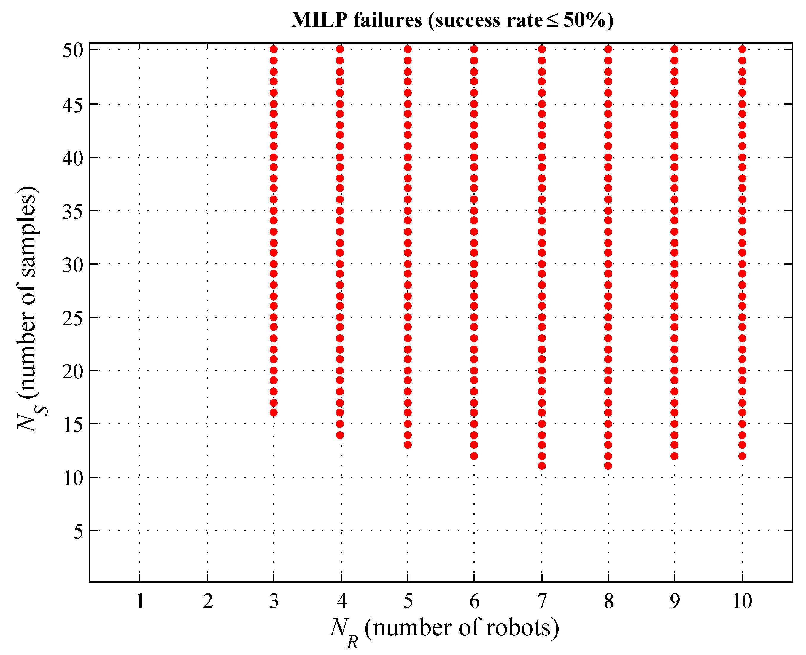
• The running time of the MILP optimization may exhibit unpredictable behaviors with respect to the team size and to the number and position of samples, leading to impossibility of obtaining a solution in some cases;
• In contrast to MILP, the running times of the QP and IH solutions have insignificant variations when small changes are made in the environment;
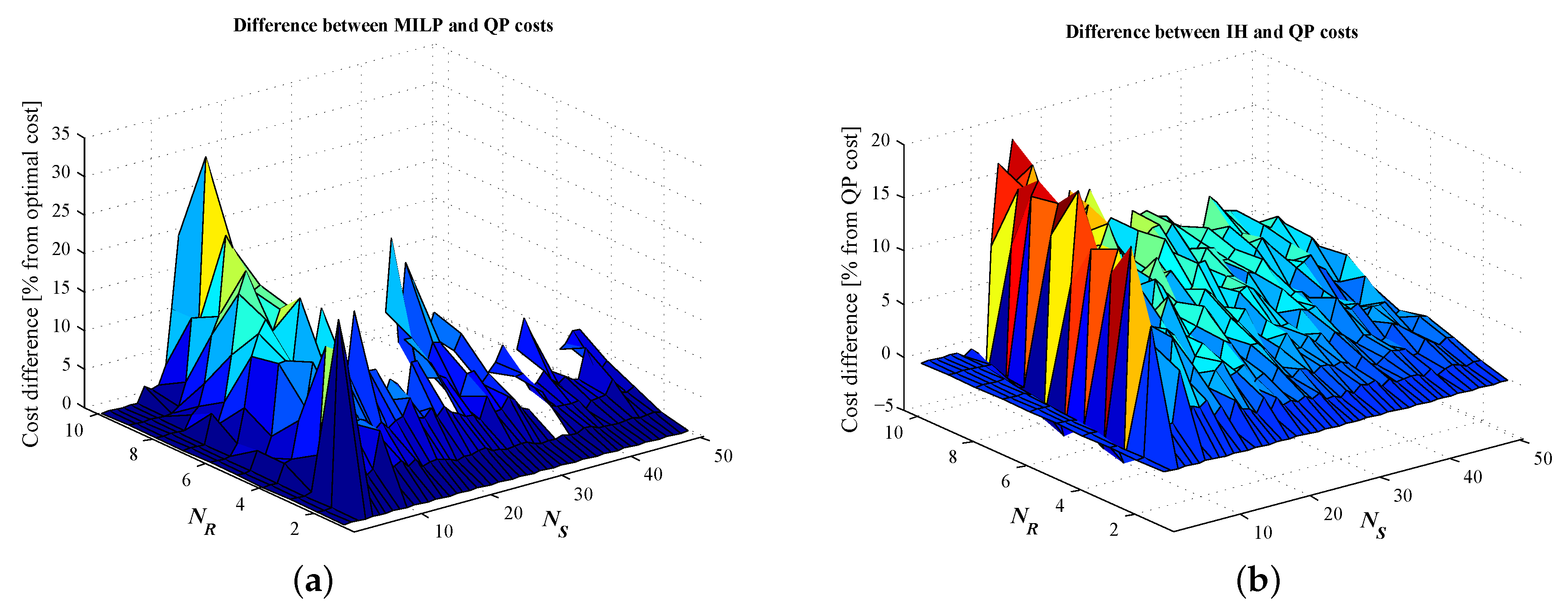
• When MILP optimization finishes, the sub-optimal costs obtained by solutions from Section 4 are generally acceptable when compared to the optimal cost;
• In some cases the QP cost was better than the one obtained by IH, while in other cases the vice versa, but again the observed differences were fairly small.

The above ideas were formulated only based on a few variations of the same example. However, they motivate the more extensive comparison performed in the next subsections between the computation feasibility and outcomes of MILP, QP, and IH solutions.

Remark 4.

As mentioned, complexity orders of MILP and QP solutions cannot be formally given. However, as is customary in some studies, we here recall the number of unknowns and constraints of these optimizations. MILP (4) and QP (8) have each $N_R\times N_S+1$ unknowns (from which $N_R\times N_S$ are binary in case of MILP (4)) and $2N_R+N_S$ linear constraints. IH solution has complexity order $\mathcal{O}(N_R\times N_S)$, based on iterative loops from Algorithm 2 but, in all our studies the execution time of the algorithm is very small.

Real-time example: Sample collecting experiments were implemented on a test-bed platform by using two Khepera robots equipped with plows for collecting items [53]. For exemplification, a movie is available at https://www.youtube.com/watch?v=2BQiWvquP7w. In the mentioned scenario, the graph environment is obtained from a cell decomposition [1,11] and a greedy method is employed for planning the robots. Although the collision avoidance problem is not treated in this paper, in the mentioned experiment the possible collisions are avoided by pausing the motion of one robot. In future work we intend to embed formal tools inspired by resource allocation techniques for collision and deadlock avoidance [54,55].

5.2. Numerical Experiments

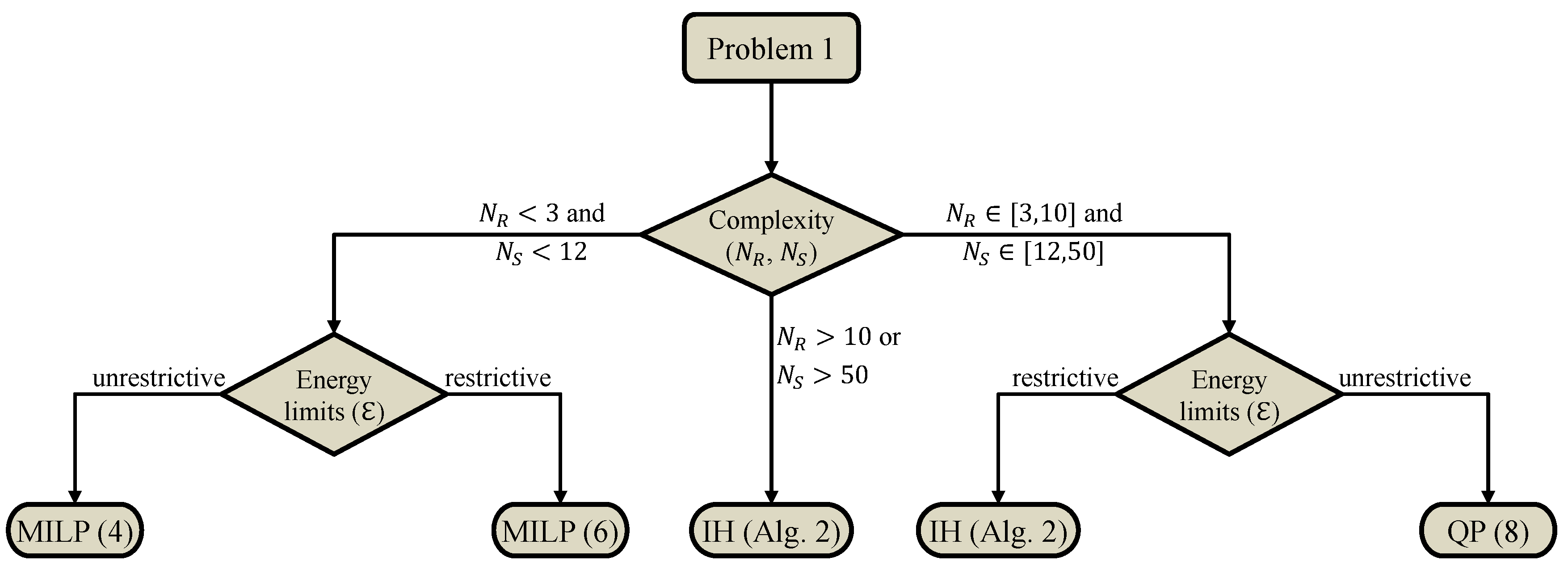
All the simulations to be presented were implemented in MATLAB [48] and were performed on a computer with Intel i7 quad-core processor and 8 GB RAM.

The numerical experiments were run for almost 15 days, and they were organized by considering the following aspects:

(i)

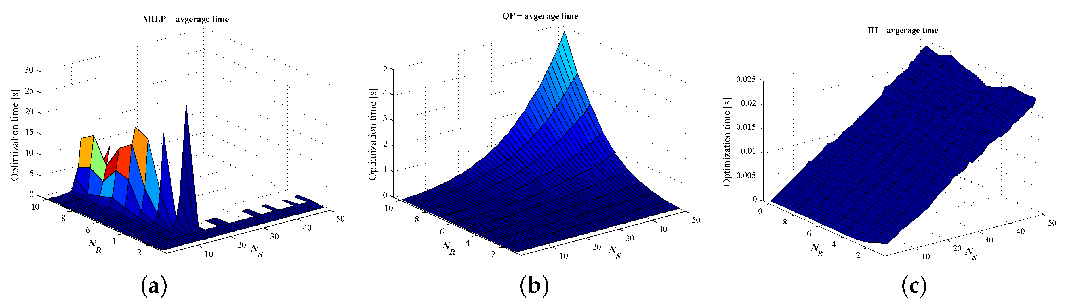
Time complexity orders cannot be a priori given for MILP or for non-convex QP optimization problems. Thus, the time for obtaining a planning solution solving Problem 1 is to be recorded as an important comparison criterion.

(ii)

The complexity of MILP, QP, and IH solutions does not directly depend on the size of environment graph G, except for the initial computation of map $\omega$ that further embeds the necessary information from the environment structure. Therefore, the running time of either solution is influenced by two parameters: the number of robots ($N_R$) and the number of samples ($N_S$).

(iii)

Based on item (ii), we consider variation ranges $(N_R,N_S)\in [2,\dots ,10]\times [2,\dots ,50]$, with unit increment steps for $N_R$ and $N_S$. Please note that the cases of 1 robot and/or 1 sample are trivial, and therefore are not included in the above parameter intervals.

(iv)

To obtain reliable results for item (i), for each pair $(N_R,N_S)$ we have run a set of 50 trials. For each trial we generated a random distribution of samples in a 50-node graph. To maintain focus on time complexity, we assumed sufficiently large amounts of robot energy $\mathcal{E}$, such that Problem 1 is not infeasible due to these limitations.

(v)

For each trial, the MILP optimization was deemed failed whenever (4) did not return a solution in less than 1 min. This is because in multiple situations we observed that if no solution is obtained in less than 30–40 s, then the MILP (4) does not finish even after 2–3 h.

(vi)

For each trial from item (iv), the QP solution was deemed failed whenever it yielded non-binary outcomes of map x (see Remark 3). The IH solution is always successful.

(vii)

For each proposed solution, for each pair $(N_R,N_S)$ from (iii) and based on trials from (iv), we computed the following comparison criteria:

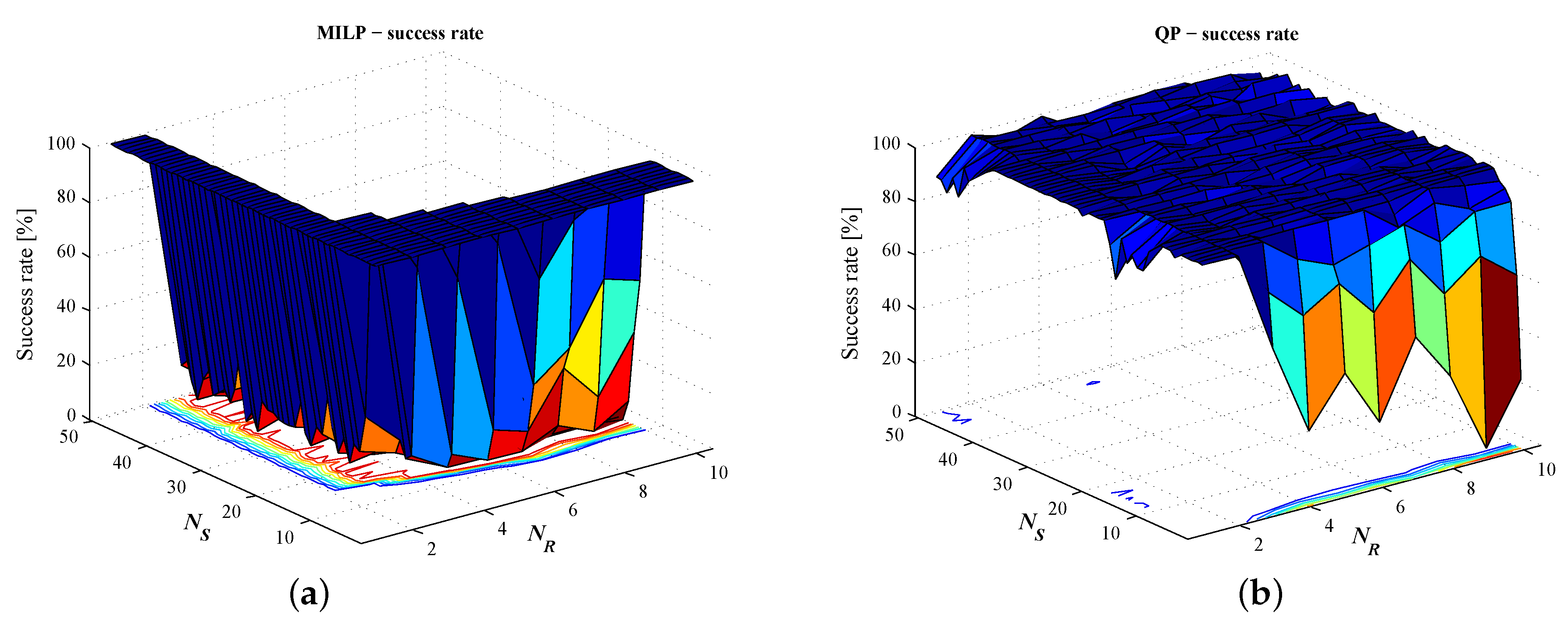
• success rate, showing the percentage of trials when the solution succeeded in outputting feasible plans;
• computation time, averaged over the successful trials of a given $(N_R,N_S)$ instance;
• solution cost, i.e., time for gathering all samples, for each successful situation.

5.3. Results

The results from item (vii) allow us to draw some rules that guide a user to choose MILP, QP, or IH solution when solving a specific instance of Problem 1. The following figures present and comment these results, leading to the decision diagram from the end of this section.

Figure 2 illustrates the success rates of the optimization problems from Section 3 and Section 4.1, respectively. For a clearer understanding, Figure 3 presents pairs $(N_R,N_S)$ when MILP (4) fails in more than $50\%$ from each set of 50 trials (see item (v) from Section 5.2). It is noted that MILP generally returns optimal solutions for small values of $N_R$ and $N_S$ and fails (because of optimization time limit) for larger values. QP returns usually returns feasible solutions, excepting some cases with small values of $N_R$ and $N_S$.

Figure 4 presents the average computation time over the successful trials, for each solution we proposed. The representation is omitted for pairs $(N_R,N_S)$ when there are less than 5 (from 50) successful trials—as it is often the case for MILP solver, when $N_R\ge 3$ and $N_S\ge 13$. MILP time may sudden variations, whereas the times for QP and IH indicates predictable behaviors. The IH time is very small (note axis limits in Figure 4) and exhibits negligible variations versus $N_R$ and almost linear increases versus $N_S$, due to the main iteration loop from Algorithm 2.

To suggest the confidence intervals of values plotted in Figure 4, we mention that:

• For $N_R=3$ and $N_S=15$, when the success rate of each optimization exceeds $98\%$, the standard deviations of optimization times are: 15 for MILP, 0.01 for QP, 0.002 for IH;
• For $N_R=10$ and $N_S=50$, when QP has $96\%$ success rate, the standard deviations of optimization times are: 0.23 for QP and 0.003 for IH.

Figure 5 presents the averaged relative differences of costs yielded by the three proposed solutions for solving Problem 1. As visible in Figure 5a, the QP (sub-optimal) cost is usually less than $120\%\dots 130\%$ of optimal MILP cost. More specifically, from all the 25,000 trials, in 8443 cases (about $33\%$) both optimizations succeeded. After averaging cost differences versus $(N_R,N_S)$, we obtained 348 points for representing Figure 5a, and in 330 cases the cost difference was less than $20\%$. Figure 5b compares the costs yielded by the sub-optimal solutions from Section 4 by representing variations of the IH cost related to the QP one. It follows that usually IH yields a higher cost than QP, but the difference decreases below $5\%\dots 10\%$ with the increase in problem complexity. Further studies can be conducted towards formulating a conjecture that gives a formal tendency for the variation of cost difference based on problem size. However, one issue for such a study is mainly given by the necessity of obtaining the optimal cost even for large problems, i.e., solving large MILP optimizations.

For more complex problems ($N_R>10$, $N_S>50$), the time tendencies from Figure 4b,c and the cost differences from Figure 5b suggest that the IH solution is preferable as a good trade-off between planning complexity and resulted cost.

Extensive simulations yielded quantitative comparison criteria. Based on this information a decision scheme Figure 6 is given for indicating the proper method to be used in a specific problem instance when a fast computation scenario is considered.

6. Conclusions

This paper details three methods for planning a team of robots such that multiple samples (items) from the environment are collected and deposited into a storage location. The environment is represented by a weighted graph, and the robots have limited amounts of energy for performing movements on this graph. The goal is to plan the agents such that the samples are collected in minimum time, under the assumption that each robot can carry at most one item at a time. The first solution is given by a MILP formulation that can be too complex to solve when there are many samples or many robots in the team. The second solution provides a QP relaxation that represents in some cases a good trade-off between the time for finding movement plans and the cost difference from the optimal one. The third solution is an IH algorithm that yields plans even when the QP fails due to low amounts of available energy for robots.

Based on the results reported in the previous subsection, the recommendations for a user that solves Problem 1 are the following: MILP (6) or IH algorithm are to be used when the robots have small amounts of energy in comparison with the energy required for moving to sample locations. Otherwise, MILP (4) and QP (8) may fail in providing any solution for such restrictive scenarios.

The usage of QP or IH solutions generally yields an acceptable loss in total time for accomplishing the mission whenever the MILP optimization becomes computationally intractable on a decently powerful computer. We emphasize that the above recommendations resulted from an intensive campaign of numerical simulations and they could not be drawn by only inspecting the formal solutions. Extensive simulations yielded quantitative comparison criteria. Based on this information a decision scheme is given for indicating the proper method to be used in a specific problem instance. Besides suggestions from Figure 6, we recall that MILP and QP solutions involve existing optimization tools.

A real-time experiment was performed for illustrating a sample gathering solution. Although the collision avoidance problem is not treated in this paper, in the mentioned experiment the possible collisions are avoided by pausing the motion of one robot. In future work we intend to embed formal tools inspired by resource allocation techniques for collision and deadlock avoidance, while considering the effects of acceleration and deceleration of the mobile robots and restricted energy.

References

1. Choset, H.; Lynch, K.; Hutchinson, S.; Kantor, G.; Burgard, W.; Kavraki, L.; Thrun, S. Principles of Robot Motion: Theory, Algorithms and Implementation; MIT Press: Cambridge, MA, USA, 2005. [Google Scholar]
2. LaValle, S.M. Planning Algorithms; Cambridge University Press: Cambridge, UK, 2006. [Google Scholar]
3. Siciliano, B.; Khatib, O. Springer Handbook of Robotics; Springer: Berlin, Germany, 2008. [Google Scholar]
4. Belta, C.; Bicchi, A.; Egerstedt, M.; Frazzoli, E.; Klavins, E.; Pappas, G.J. Symbolic Planning and Control of Robot Motion. IEEE Robot. Autom. Mag. 2007, 14, 61–71. [Google Scholar] [CrossRef]
5. Imeson, F.; Smith, S.L. A Language For Robot Path Planning in Discrete Environments: The TSP with Boolean Satisfiability Constraints. In Proceedings of the IEEE Conference on Robotics and Automation, Hong Kong, China, 31 May–7 June 2014; pp. 5772–5777. [Google Scholar]
6. Mahulea, C.; Kloetzer, M. Robot Planning based on Boolean Specifications using Petri Net Models. IEEE Trans. Autom. Control 2018, 63, 2218–2225. [Google Scholar] [CrossRef]
7. Fainekos, G.; Girard, A.; Kress-Gazit, H.; Pappas, G. Temporal logic motion planning for dynamic robot. Automatica 2009, 45, 343–352. [Google Scholar] [CrossRef]
8. Ding, X.; Lazar, M.; Belta, C. {LTL} receding horizon control for finite deterministic systems. Automatica 2014, 50, 399–408. [Google Scholar] [CrossRef]
9. Schillinger, P.; Bürger, M.; Dimarogonas, D. Simultaneous task allocation and planning for temporal logic goals in heterogeneous multi-robot systems. Int. J. Robot. Res. 2018, 37, 818–838. [Google Scholar] [CrossRef] [Green Version]
10. Kloetzer, M.; Mahulea, C. LTL-Based Planning in Environments With Probabilistic Observations. IEEE Trans. Autom. Sci. Eng. 2015, 12, 1407–1420. [Google Scholar] [CrossRef]
11. Berg, M.D.; Cheong, O.; van Kreveld, M. Computational Geometry: Algorithms and Applications, 3rd ed.; Springer: Berlin, Germany, 2008. [Google Scholar]
12. Kloetzer, M.; Mahulea, C. A Petri net based approach for multi-robot path planning. Discret. Event Dyn. Syst. 2014, 24, 417–445. [Google Scholar] [CrossRef]
13. Cassandras, C.; Lafortune, S. Introduction to Discrete Event Systems; Springer: Berlin, Germany, 2008. [Google Scholar]
14. Silva, M. Introducing Petri nets. In Practice of Petri Nets in Manufacturing; Springer: Berlin, Germany, 1993; pp. 1–62. [Google Scholar]
15. Burkard, R.; Dell’Amico, M.; Martello, S. Assignment Problems; SIAM e-Books; Society for Industrial and Applied Mathematics (SIAM): Philadelphia, PA, USA, 2009. [Google Scholar]
16. Mosteo, A.; Montano, L. A Survey of Multi-Robot Task Allocation; Technical Report AMI-009-10-TEC; Instituto de Investigación en Ingenierıa de Aragón, University of Zaragoza: Zaragoza, Spain, 2010. [Google Scholar]
17. Gerkey, B.; Matarić, M. A formal analysis and taxonomy of task allocation in multi-robot systems. Int. J. Robot. Res. 2004, 23, 939–954. [Google Scholar] [CrossRef]
18. Korsah, G.; Stentz, A.; Dias, M. A comprehensive taxonomy for multi-robot task allocation. Int. J. Robot. Res. 2013, 32, 1495–1512. [Google Scholar] [CrossRef]
19. Shmoys, D.; Tardos, É. An approximation algorithm for the generalized assignment problem. Math. Program. 1993, 62, 461–474. [Google Scholar] [CrossRef]
20. Atay, N.; Bayazit, B. Emergent task allocation for mobile robots. In Proceedings of the Robotics: Science and Systems, Atlanta, GA, USA, 27–30 June 2007. [Google Scholar]
21. Cardema, J.; Wang, P. Optimal Path Planning of Multiple Mobile Robots for Sample Collection on a Planetary Surface. In Mobile Robots: Perception & Navigation; Kolski, S., Ed.; IntechOpen: London, UK, 2007; pp. 605–636. [Google Scholar]
22. Chen, J.; Sun, D. Coalition-Based Approach to Task Allocation of Multiple Robots with Resource Constraints. IEEE Trans. Autom. Sci. Eng. 2012, 9, 516–528. [Google Scholar] [CrossRef]
23. Das, G.; McGinnity, T.; Coleman, S.; Behera, L. A Distributed Task Allocation Algorithm for a Multi-Robot System in Healthcare Facilities. J. Intell. Robot. Syst. 2015, 80, 33–58. [Google Scholar] [CrossRef]
24. Burger, M.; Notarstefano, G.; Allgower, F.; Bullo, F. A distributed simplex algorithm and the multi-agent assignment problem. In Proceedings of the American Control Conference (ACC), San Francisco, CA, USA, 29 June–1 July 2011; pp. 2639–2644. [Google Scholar]
25. Luo, L.; Chakraborty, N.; Sycara, K. Multi-robot assignment algorithm for tasks with set precedence constraints. In Proceedings of the IEEE International Conference on Robotics and Automation (ICRA), Shanghai, China, 9–13 May 2011; pp. 2526–2533. [Google Scholar]
26. Toth, P.; Vigo, D. (Eds.) The Vehicle Routing Problem; Society for Industrial and Applied Mathematics: Philadelphia, PA, USA, 2001. [Google Scholar]
27. Laporte, G.; Nobert, Y. Exact Algorithms for the Vehicle Routing Problem. In Surveys in Combinatorial Optimization; Martello, S., Minoux, M., Ribeiro, C., Laporte, G., Eds.; North-Holland Mathematics Studies; North-Holland: Amsterdam, The Netherlands, 1987; Volume 132, pp. 147–184. [Google Scholar]
28. Toth, P.; Vigo, D. Models, relaxations and exact approaches for the capacitated vehicle routing problem. Discret. Appl. Math. 2002, 123, 487–512. [Google Scholar] [CrossRef] [Green Version]
29. Raff, S. Routing and scheduling of vehicles and crews: The state of the art. Comput. Oper. Res. 1983, 10, 63–211. [Google Scholar] [CrossRef]
30. Christofides, N. Vehicle routing. In The Traveling Salesman Problem: A guided Tour of Combinatorial Optimization; Wiley: New York, NY, USA, 1985; pp. 410–431. [Google Scholar]
31. Laporte, G. The vehicle routing problem: An overview of exact and approximate algorithms. Eur. J. Oper. Res. 1992, 59, 345–358. [Google Scholar] [CrossRef]
32. Chen, J.F.; Wu, T.H. Vehicle routing problem with simultaneous deliveries and pickups. J. Oper. Res. Soc. 2006, 57, 579–587. [Google Scholar] [CrossRef]
33. Kloetzer, M.; Burlacu, A.; Panescu, D. Optimal multi-agent planning solution for a sample gathering problem. In Proceedings of the IEEE International Conference on Automation, Quality and Testing, Robotics (AQTR), Cluj-Napoca, Romania, 22–24 May 2014. [Google Scholar]
34. Kloetzer, M.; Ostafi, F.; Burlacu, A. Trading optimality for computational feasibility in a sample gathering problem. In Proceedings of the International Conference on System Theory, Control and Computing, Sinaia, Romania, 17–19 October 2014; pp. 151–156. [Google Scholar]
35. Kloetzer, M.; Mahulea, C. An Assembly Problem with Mobile Robots. In Proceedings of the IEEE 19th Conference on Emerging Technologies Factory Automation, Barcelona, Spain, 16–19 September 2014. [Google Scholar]
36. Panescu, D.; Kloetzer, M.; Burlacu, A.; Pascal, C. Artificial Intelligence based Solutions for Cooperative Mobile Robots. J. Control Eng. Appl. Inform. 2012, 14, 74–82. [Google Scholar]
37. Kloetzer, M.; Mahulea, C.; Burlacu, A. Sample gathering problem for different robots with limited capacity. In Proceedings of the International Conference on System Theory, Control and Computing, Sinaia, Romania, 13–15 October 2016; pp. 490–495. [Google Scholar]
38. Tumova, J.; Dimarogonas, D. Multi-agent planning under local LTL specifications and event-based synchronization. Automatica 2016, 70, 239–248. [Google Scholar] [CrossRef] [Green Version]
39. Belta, C.; Habets, L. Constructing decidable hybrid systems with velocity bounds. In Proceedings of the 43rd IEEE Conference on Decision and Control, Nassau, Bahamas, 14–17 December 2004; pp. 467–472. [Google Scholar]
40. Habets, L.C.G.J.M.; Collins, P.J.; van Schuppen, J.H. Reachability and control synthesis for piecewise-affine hybrid systems on simplices. IEEE Trans. Autom. Control 2006, 51, 938–948. [Google Scholar] [CrossRef]
41. Garey, M.; Johnson, D. “Strong” NP-Completeness Results: Motivation, Examples, and Implications. J. ACM 1978, 25, 499–508. [Google Scholar] [CrossRef]
42. Cormen, T.; Leiserson, C.; Rivest, R.; Stein, C. Introduction to Algorithms, 2nd ed.; MIT Press: Cambridge, MA, USA, 2001. [Google Scholar]
43. Ding-Zhu, D.; Pardolos, P. Nonconvex Optimization and Applications: Minimax and Applications; Spinger: New York, NY, USA, 1995. [Google Scholar]
44. Polak, E. Optimization: Algorithms and Consistent Approximations; Spinger: New York, NY, USA, 1997. [Google Scholar]
45. Floudas, C.; Pardolos, P. Encyclopedia of Optimization, 2nd ed.; Spinger: New York, NY, USA, 2009; Volume 2. [Google Scholar]
46. Makhorin, A. GNU Linear Programming Kit. 2012. Available online: http://www.gnu.org/software/glpk/ (accessed on 4 January 2019).
47. SAS Institute. The Mixed-Integer Linear Programming Solver. 2014. Available online: http://support.sas.com/rnd/app/or/mp/MILPsolver.html (accessed on 4 January 2019).
48. The MathWorks. MATLAB®R2014a (v. 8.3); The MathWorks: Natick, MA, USA, 2006. [Google Scholar]
49. Wolsey, L.; Nemhauser, G. Integer and Combinatorial Optimization; Wiley: New York, NY, USA, 1999. [Google Scholar]
50. Vazirani, V.V. Approximation Algorithms; Springer: New York, NY, USA, 2001. [Google Scholar]
51. Earl, M.; D’Andrea, R. Iterative MILP Methods for Vehicle-Control Problems. IEEE Trans. Robot. 2005, 21, 1158–1167. [Google Scholar] [CrossRef]
52. Murray, W.; Ng, K. An Algorithm for Nonlinear Optimization Problems with Binary Variables. Comput. Optim. Appl. 2010, 47, 257–288. [Google Scholar] [CrossRef]
53. Tiganas, V.; Kloetzer, M.; Burlacu, A. Multi-Robot based Implementation for a Sample Gathering Problem. In Proceedings of the International Conference on System Theory, Control and Computing, Sinaia, Romania, 11–13 October 2013; pp. 545–550. [Google Scholar]
54. Kloetzer, M.; Mahulea, C.; Colom, J.M. Petri net approach for deadlock prevention in robot planning. In Proceedings of the IEEE Conference on Emerging Technologies Factory Automation (ETFA), Cagliari, Italy, 10–13 September 2013; pp. 1–4. [Google Scholar]
55. Roszkowska, E.; Reveliotis, S. A Distributed Protocol for Motion Coordination in Free-Range Vehicular Systems. Automatica 2013, 49, 1639–1653. [Google Scholar] [CrossRef]
Figure 1. Example: environment graph with 10 nodes, 3 robots, and 14 samples. The robot moving costs are marked on graph edges, and the samples are represented by the blue discs.
Applsci 09 00791 g001
Figure 2. Success rates of MILP (a) and QP (b) vs. number of robots N R and number of samples N S .
Applsci 09 00791 g002
Figure 3. MILP (4): 2D projection for failures, defined as success rate of less than 50 % .
Applsci 09 00791 g003
Figure 4. Average optimization times, for ( N R , N S ) pairs for which at least 5 feasible solutions from the 50 tests were obtained: (a) MILP (4), (b) QP (8), (c) IH from Algorithm 2.
Applsci 09 00791 g004
Figure 5. Differences between costs induced by the three solutions: (a) difference between QP and MILP costs, related to the optimal MILP cost; (b) difference between IH and QP sub-optimal costs, related to QP cost.
Applsci 09 00791 g005
Figure 6. Decision diagram for choosing an appropriate solution for Problem 1 when a fast computational scenario is considered.
Applsci 09 00791 g006