Generative Oversampling Method for Imbalanced Data on Bearing Fault Detection and Diagnosis

Abstract

In this study, we developed a novel data-driven fault detection and diagnosis (FDD) method for bearing faults in induction motors where the fault condition data are imbalanced. First, we propose a bearing fault detector based on convolutional neural networks (CNN), in which the vibration signals from a test bench are used as inputs after an image transformation procedure. Experimental results demonstrate that the proposed classifier for FDD performs well (accuracy of 88% to 99%) even when the volume of normal and fault condition data is imbalanced (imbalance ratio varies from 20:1 to 200:1). Additionally, our generative model reduces the level of data imbalance by oversampling. The results improve the accuracy of FDD (by up to 99%) when a severe imbalance ratio (200:1) is assumed.

1. Introduction

Fault detection and diagnosis (FDD) in manufacturing facilities is very important for (1) improving productivity by preventing undesired downtime and (2) guaranteeing safe working conditions [1]. Traditional FDD methods were developed using physical models based on mathematics and mechatronics [2,3,4,5,6]. Those methods require complex analysis steps with domain knowledge. In addition, because physical models are highly dependent on individual specifications, user configuration is needed when the model is used in a specific facility. To overcome the problems of physical models, assorted data-driven FDD methods that use machine learning and statistics, such as support vector machine [7,8] and fuzzy logic [9], have been proposed. However, these data-driven FDDs still require a complicated pre-processing step before training of the models.

Recently, deep neural networks (DNNs) with more powerful fitting abilities have been developed and widely applied to prognostics and health management. In [10,11,12,13,14,15], time-domain and frequency-domain features are extracted in data processing, and then an FDD model is applied for motor status classification. In [16,17,18], vibration image generation with signal analysis was utilized for feature extractions. The feature extraction method itself can be automated using these approaches, but establishing such models requires complicated signal processing steps. Automatic feature extraction using an auto-encoder has been proposed [19], but the computation cost of the DNN model itself is quite high. To realize wide adoption of data-driven FDD to industry, simpler and more efficient methods are required in both data-processing and DNN models.

Furthermore, these data-driven methods have shown great performance with low domain knowledge requirements, but problems related to the quantity and quality of data still remain. Data imbalance is common in FDD because normal condition data are more prevalent than faulty condition data in real manufacturing environments [20]. Such imbalanced conditions degrade data-driven FDD, especially for convolutional neural network (CNN)-based classifiers. Among oversampling [11,21], down-sampling [22], and ensemble learning [23], all of which have been proposed to solve the data imbalance issue, oversampling is most suitable for industrial FDD because of severe data imbalance ratios. Additionally, oversampling is always the most effective way to deal with class imbalance for the CNN model on image classification [24].

In this study, we investigated the data-driven FDD of bearing faults in an induction motor under data imbalance conditions. Firstly, a CNN based classifier with an imaging method for vibration signals was proposed. We utilized the nested scatter plot (NSP) [25], which is an efficient and scalable image transformation of correlated time-series data. In NSP, the correlated time-series data are represented by a square matrix, similar to a scatter plot, where the elements of density dots are calculated like a heat-map. Experimental evaluation using measured vibration signals from a test bench confirmed that the features of bearing faults are easily extracted using NSP and the CNN-classifier.

Secondly, an oversampling method with a generative model was proposed to improve performance when a dataset is imbalanced between normal and faulty conditions. The generative model was developed based on a Wasserstein generative adversarial network with a gradient penalty (WGAN-GP) [26] and deep convolutional generative adversarial networks (DCGAN) [27]. We evaluated the performance improvement of the CNN classifier for various conditions after applying our oversampling method to faulty condition data.

The remainder of this paper is organized as follows: Section 2 introduces the proposed data-driven fault detection method. Section 3 presents the generative model based on WGAN-GP and DCGAN. We describe our experiment method and its results in Section 4. The conclusions and future research topics are discussed in Section 5.

2. Data-Driven Bearing Fault Detection

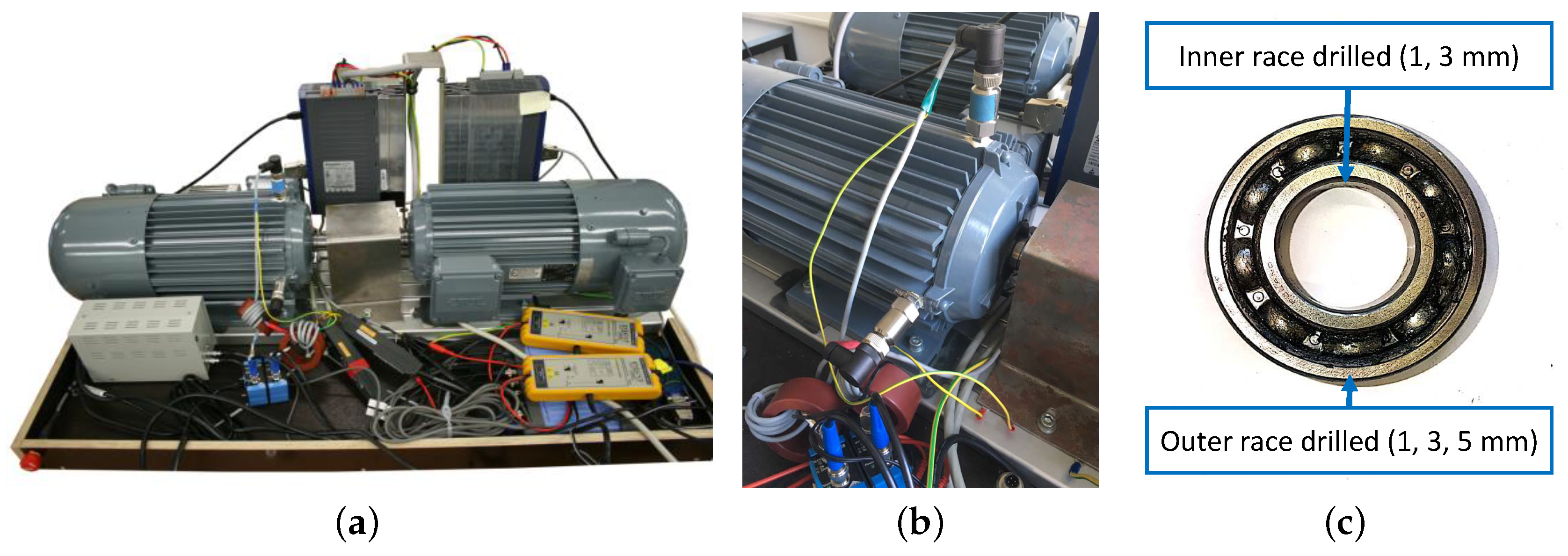
2.1. Data Collection

The purpose of our fault detection method was to detect bearing faults and diagnose the fault types. Among the various fault types, inner race, outer race, and contaminant faults were considered. As an initial step, we collected two channels (the horizontal and vertical axes) of vibration signals for normal and faulty conditions using the apparatus shown in Figure 1a.

The motors of the test bench were 3 kW three-phase induction motors with rated voltage 400 V and current 6.4 A. The configuration followed the power drive setup in [28]. We connected the motors to the controller via inverters to control the speed and torque. The running environment had a $25\mathrm{Hz}$ operation frequency and $10$Nm torque. The motors and inverters were mounted on the steel rail to fix the electronic machines.

For data acquisition, two vibration sensors (model: MMF KS80D, range: $\pm 60$g, bandwidth $22\mathrm{kHz}$, sensitivity: $0.1$V/g) were used to record vibration in the x- and z-axis (as shown in Figure 1b). An oscilloscope was connected to vibration sensors and the recorded vibration signals were stored in a server. In our experiments, the sampling rate of the vibration signal was $1\mathrm{MHz}$. Vibration data from the induction motor were collected from the test bench under varying environment conditions over the course of a year.

To measure faulty condition data, bearings were artificially damaged by the following methods. For inner and outer race faults, we drilled into the middle of the inner and outer raceway in the bearings after removing the metal shield and the grease in the bearing. The drilling diameter was 1, 3, and 5 mm for low, medium, and high severity, respectively. For the contaminant, we inserted metal chips in the cage. The bearing with different faulty conditions is shown in Figure 1c.

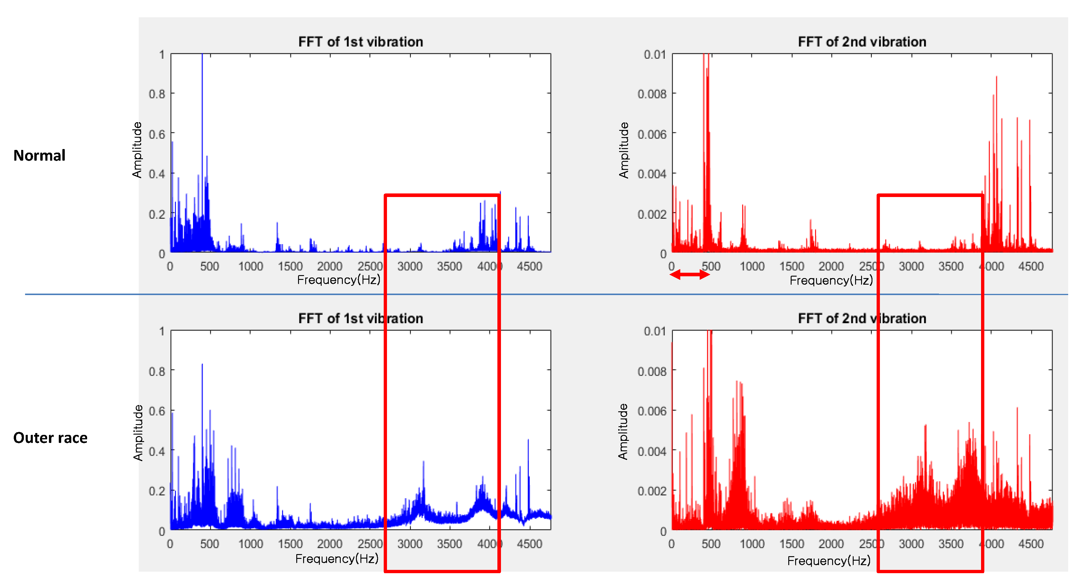
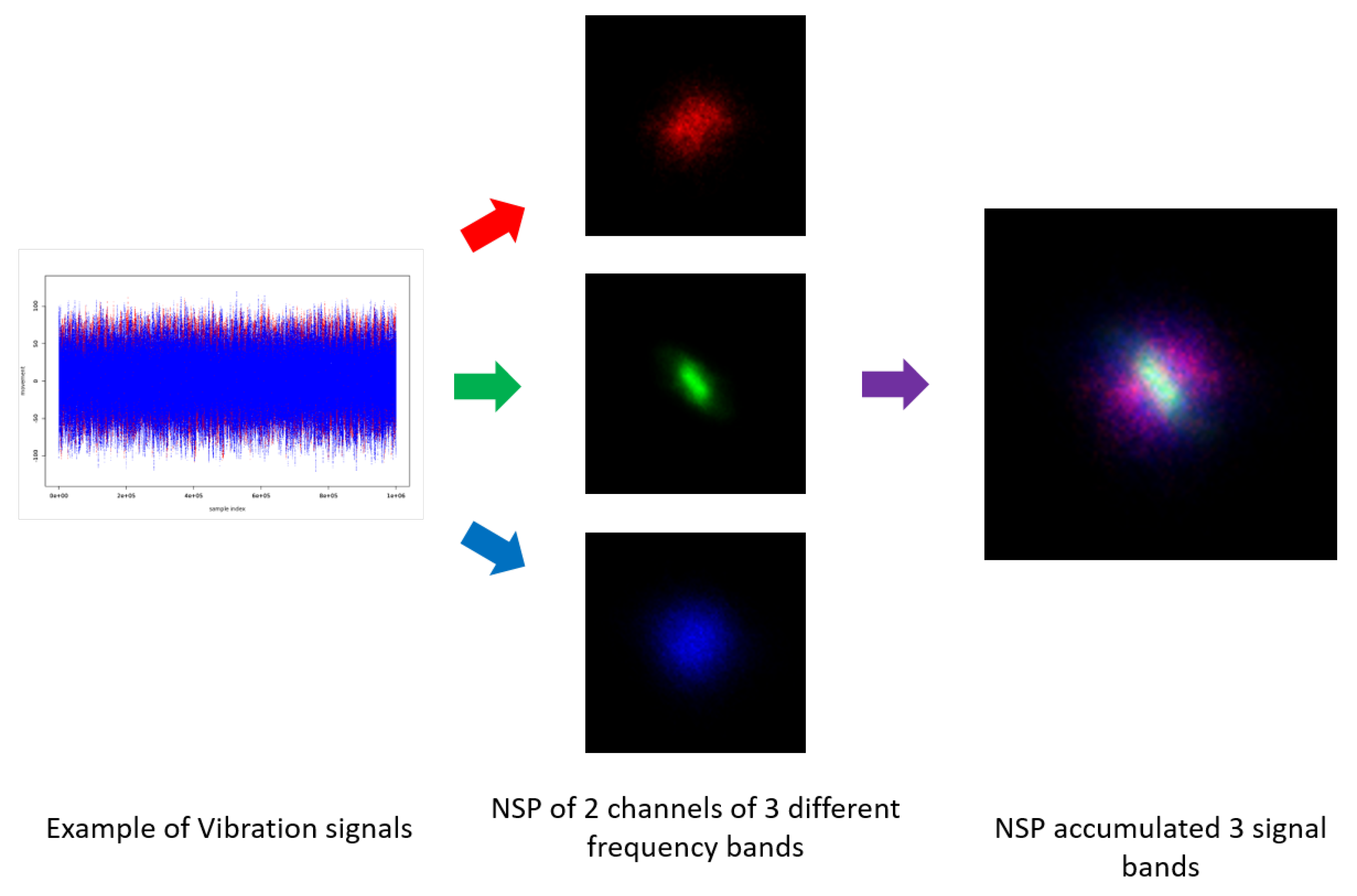
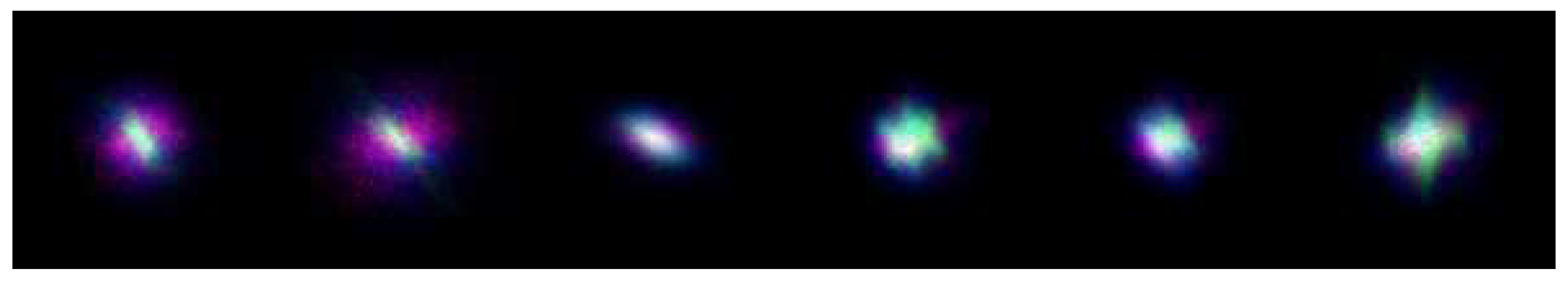
2.2. Image Transformation of Vibration Signals

NSP [25] is a data wrangling method that uses image transformation of correlated time series data for multi-variate correlation analysis and machine learning. Multi-channel signals are represented in fixed-size images that are generated through three steps: compression in nested clusters, imaging, and accumulating (Figure 2). The first step was compression in the nested clusters, in which the values of time-series data with a given range were mapped into a cluster, and each cluster held a count of mapped values. In the imaging step, a scatter plot was drawn for the multi-channel nested clusters with given colors. To sustain the fixed image size, the sizes of the clusters for each channel signal were controlled. To represent the intensity of each cluster in the time-series data, the count of mapped values was translated into pixel intensity. In the accumulating step, multiple sets of correlated signals were concatenated as a single RGB image.

In [11], signal processing techniques such as the Hilbert–Huang transformation (HHT) and wavelet transform were employed for vibration signal decomposition to detect bearing faults. We also exploited NSP representation of vibration signals for bearing fault detection (denoted as BF-NSP), but using a simpler decomposition method. Specifically, we extracted signals in different bandwidths from the vibration data and represented them with different colors in a single image.

Selecting the bandwidths of decomposition is important. In [29], faulty condition data showed high spectral density in a high-frequency band (30 to 40 kHz), known as the resonance band. Our analysis also showed that the spectral density for 25 to 40 kHz of faulty condition data was greater than that of normal condition data (Figure 3). In this study, BF-NSP used three bandpass filters: 10 to 30 kHz, 30 to 50 kHz, and 0 to 250 kHz.

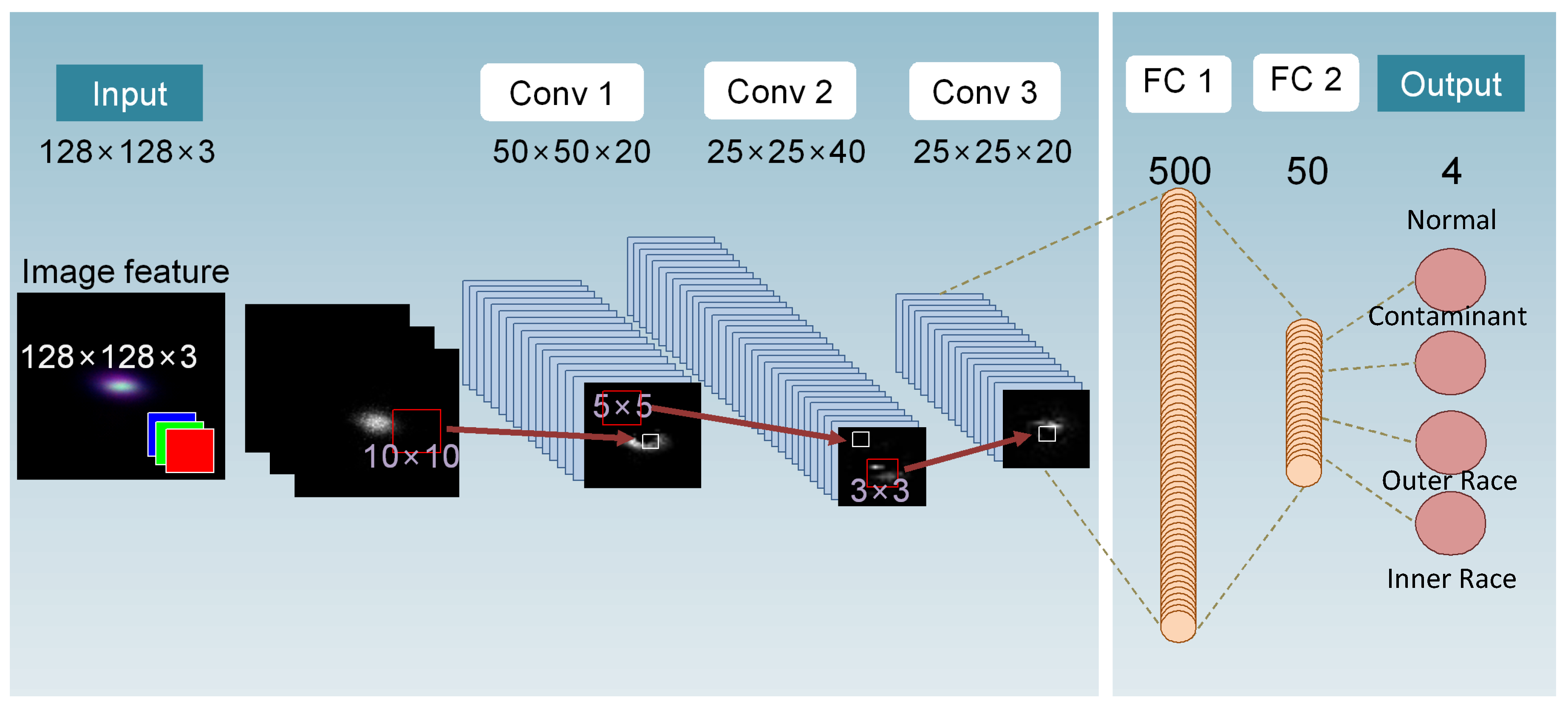
2.3. Fault Classification Using CNN

Using BF-NSP, solving FDD problems by time-series data analysis becomes an image recognition problem. We employ a CNN classifier because it provides outstanding performance in image recognition and classification [11]. The structure of the proposed CNN classifier, the CNN-based bearing fault detector (CBFD), is shown in Figure 4. There are three convolution (Conv) layers with kernel size $10\times 10$, $5\times 5$, and $3\times 3$, respectively. Batch normalization was applied to the first Conv layer only. Two fully connected (FC) layers followed the Conv layers. Output nodes reflected fault types; there were four output nodes for the normal condition and three bearing fault types (inner race, outer race, and contaminant fault). The activation functions for all layers were ReLU.

In the CNN architecture, the selectable hyper parameters were the number of filters in each Conv layer, the size of each FC layer, and dropout rate. To determine the hyper parameters, the criteria for the fault classifier under data imbalanced condition was defined as accuracy over 95% for test sets in mild imbalance ratio less than 20:1 and high accuracy even in cases of severe imbalance ratio over 50:1.

We tested varying the number of filters in each Conv layer and found the optimal numbers that met the criteria of training and test accuracy. The results of the number of filters should range from 10 to 50 because underfitting occurred when the number of filters was less than 10 and overfitting occurred when it was more than 50. The size of the FC layer affected the expressiveness of the networks and the training time. A large FC layer size increased the risk of overfitting and training time but could increase the accuracy. Through our experimentation, two FC layers of sizes less than 200 and 20 could not meet our performance criteria. Considering the overfitting and the training time, the optimal size of each FC layer was determined as 500 and 50. Finally, a dropout layer with 75% keep probability was applied to the first FC layer to mitigate overfitting in the training phase. The CBFD model is described in Figure 4.

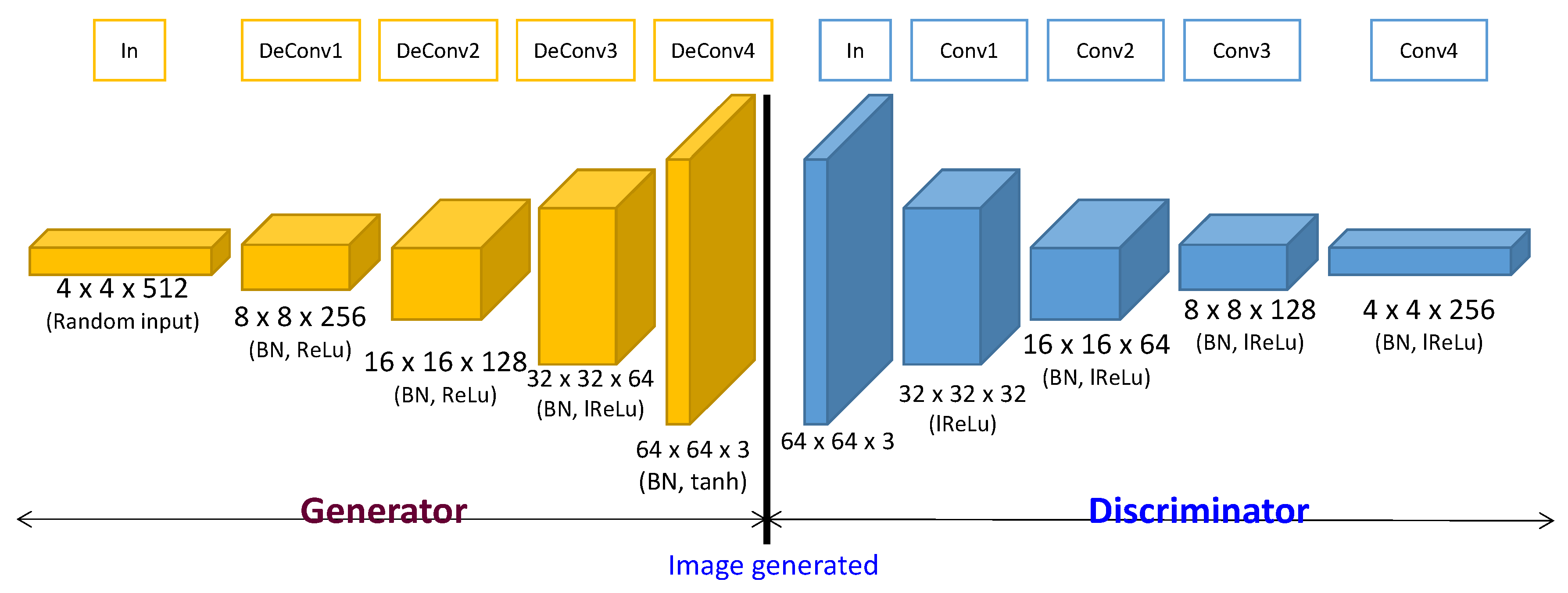
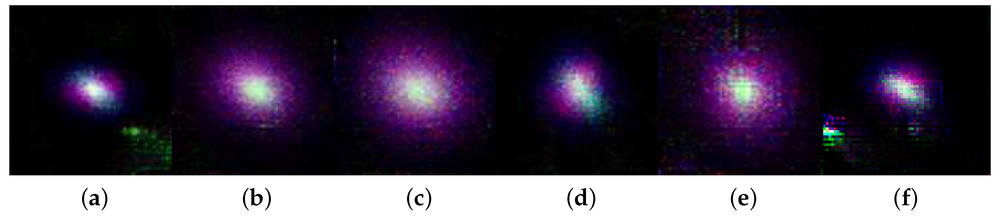
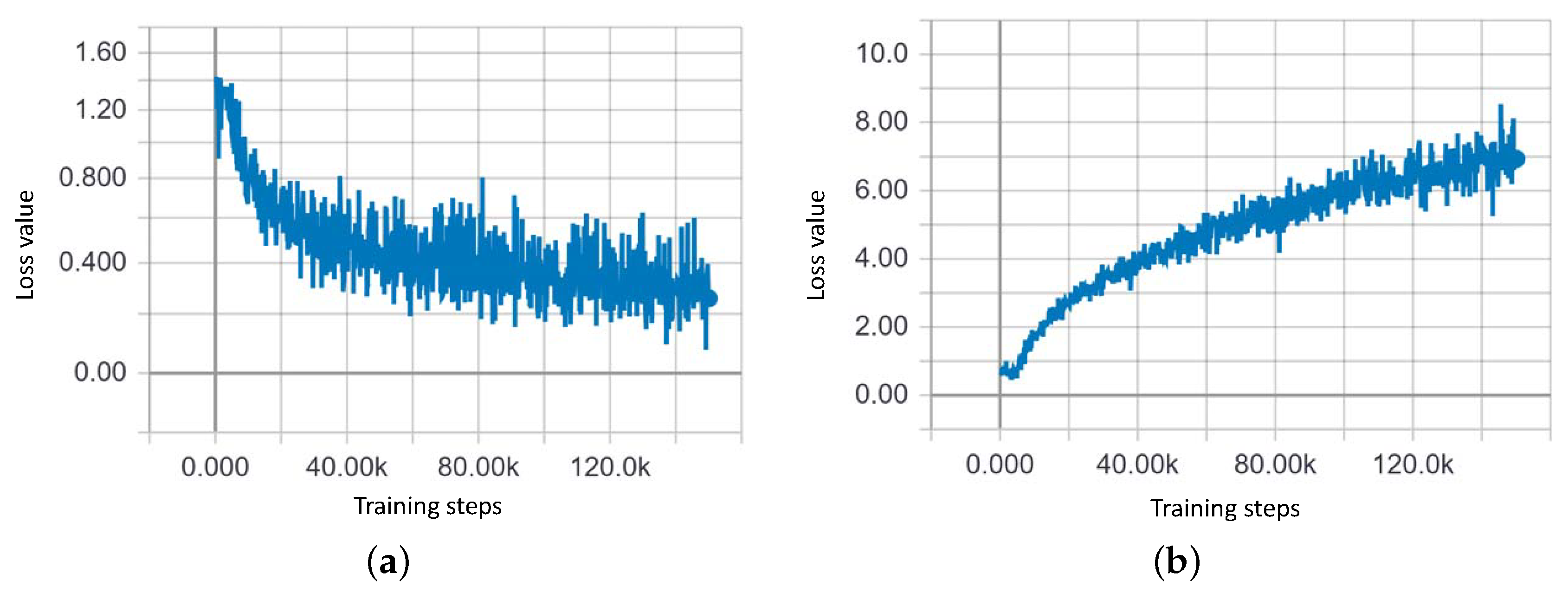
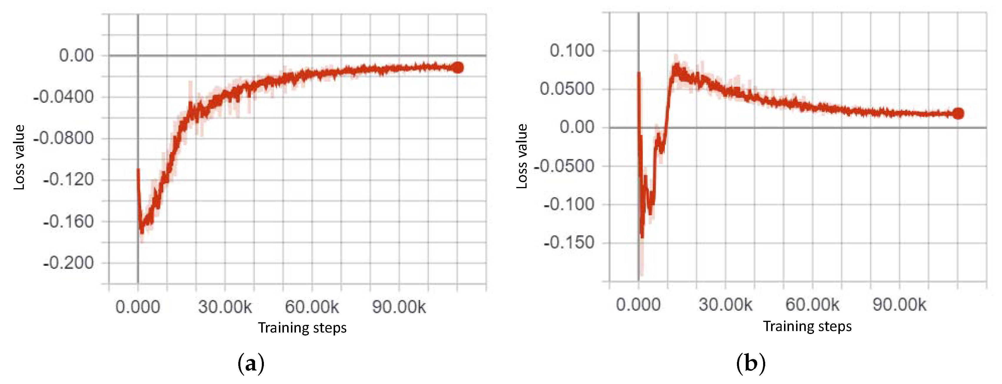
3. Generative Model for Oversampling Fault Condition Data

The performance of FDD heavily depended on the designated frequency bands in BF-NSP and the architecture of the CBFD model. However, here, we emphasize the training method used for the data-imbalance conditions.

CNN-based classification performs well when the distribution of classes is roughly balanced. However, faulty condition data are generally lower in volume than normal condition data [20]. Such imbalances cause lower recognition accuracy for the minor class, in this case the faulty condition data. This phenomenon is important because the recognition rate of faulty conditions is the most important practical measure of effective FDD in engineering applications [30].

There are three solution types for data imbalance: oversampling [11,21], down-sampling [22], and ensemble learning [23]. For extreme cases such as rare occurrence fault condition data, oversampling was the most suitable approach. In contrast, reducing the size of the entire dataset by down-sampling and modeling of the minor data can cause a lack of data and make training itself impossible.

To solve the data-imbalance problem in FDD, we considered a generative oversampling method. Oversampling with generative adversarial networks (GANs) improved FDD accuracy in a previous study [11].

GANs [31] represent a class of generative models based on a game theory scenario in which a generator network G competes against an adversary D, a discriminator. DCGAN [27] is an extended model of GAN that uses de-convolution layers in the generator and convolution layers in the discriminator to extract features of images and construct a model to generate realistic fake images. By using DCGAN, BF-NSP can be generated and used for oversampling. Figure 5 shows the DCGAN architecture employed in this study, in which we considered the convergence problem of DCGAN.

GANs aim to approximate the probability distribution function that the input data are assumed to be drawn from. In the original formulation of GANs [31], it was achieved by treating the discriminator as a binary classifier for real and fake data distributions. In this way, the discriminator provides meaningful gradients for the generator so that it minimizes the Jensen–Shannon (JS) divergence between the real and fake data distributions. However, this process is shown to be extremely unstable and difficult to train in practice. It has been shown that even in considerably simple scenarios the JS divergence does not supply useful gradients for the generator [32]. For this reason, numerous recent studies have focused on improving the stability and performance of GANs by enhancing the quality of the gradients derived from the discriminator.

To stabilize our generative model, we propose WGAN-GP [26] on the DCGAN architecture model (DCWGAN-GP). The original WGAN [32] exploited earth mover’s distance (EMD) as a better means to measure the similarity between the two distributions. In this way, the losses of the discriminator and the generator correlate well with the output image quality. WGAN-GP utilizes the same distance measurement but ensures higher stability by penalizing the norm of the discriminator’s output with respect to its input data. Our DCWGAN-GP is therefore resilient to the vanishing gradients problem and generates realistic fake images in a stable manner.

When input data are imbalanced, minor data are oversampled by the generative model until the desired ratio is met; at this point, we trained the CBFD model.

4. Experimental Results

4.1. Data Preparation and Runtime Environment

We transformed the sensor data into the image domain using BF-NSP. The sensor data were collected under various circumstances. Figure 6 shows normal data under various circumstances, with the range of images being very broad. In Figure 7, each image shows a fault type that can be distinguished by comparison with the normal image.

Table 1. Image data sets for motor condition.

Type		No. of Images
Normal		21,000
Contaminant		800
Inner Race	High	1000
	Mid	1000
Outer Race	High	1000
	Mid	1000
	Low	1000

describes the detailed dataset for each operating condition. To verify the capability of FDD in data imbalanced condition, the number of images for normal conditions was much greater than the number of images of bearing faults.

The proposed fault detection and generative networks were implemented using Python scripts on the TensorFlow framework. The implemented NSP representation, CNN classifier, and generative networks were tested on a Linux system. The details of the runtime environment are shown in

Table 2. Runtime environment details.

Category	Specification
CPU	Intel Core i7-7700K
RAM	64GB DDR4 memory
GPU	NVIDIA Titan XP 12GB GDDR5X
OS	Ubuntu 16.04 LTS (Linux)
SW libraries	Python 3.4/CUDA v8.0/ cuDNN v6.0/Tensorflow r1.4

.

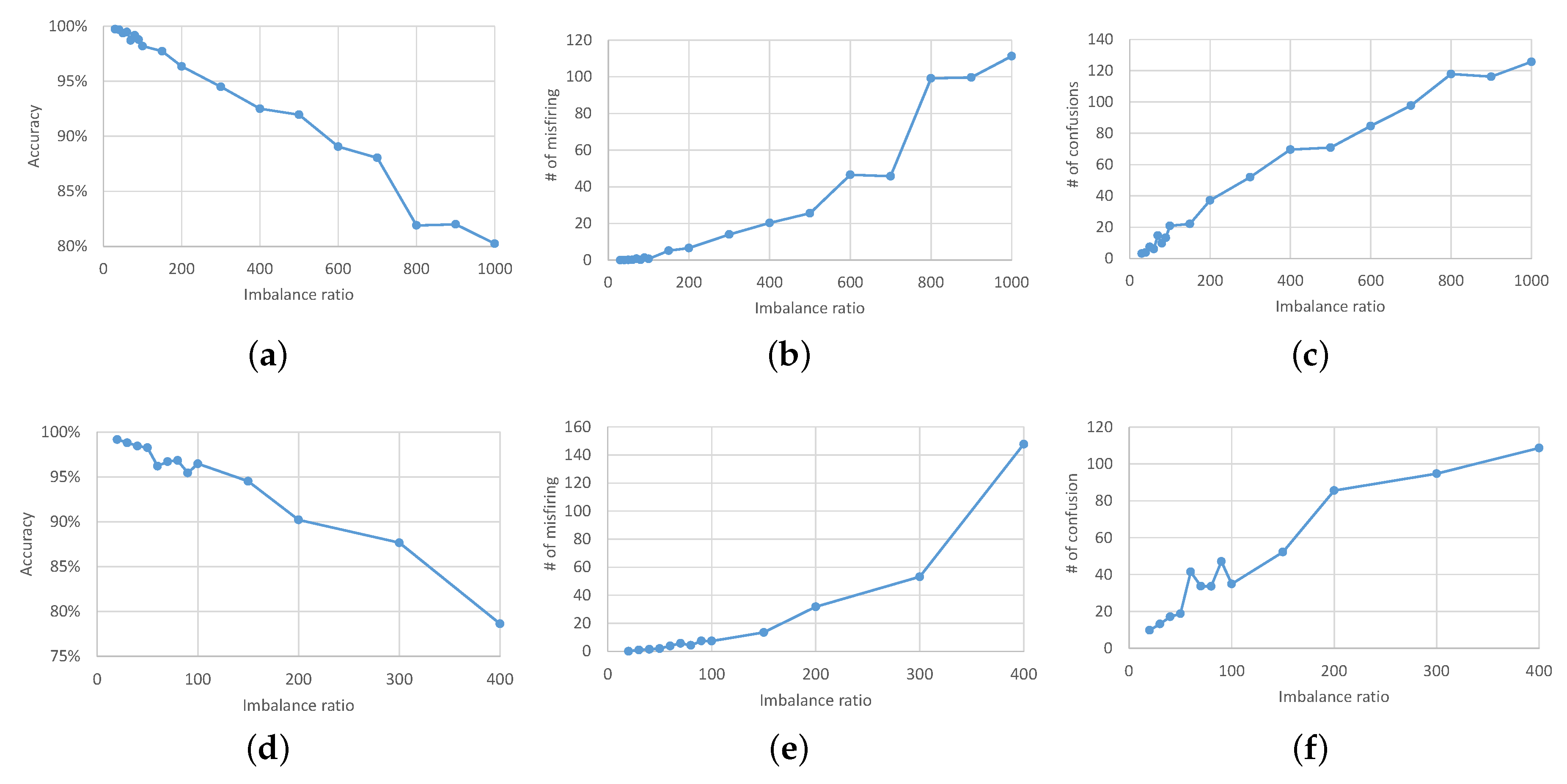
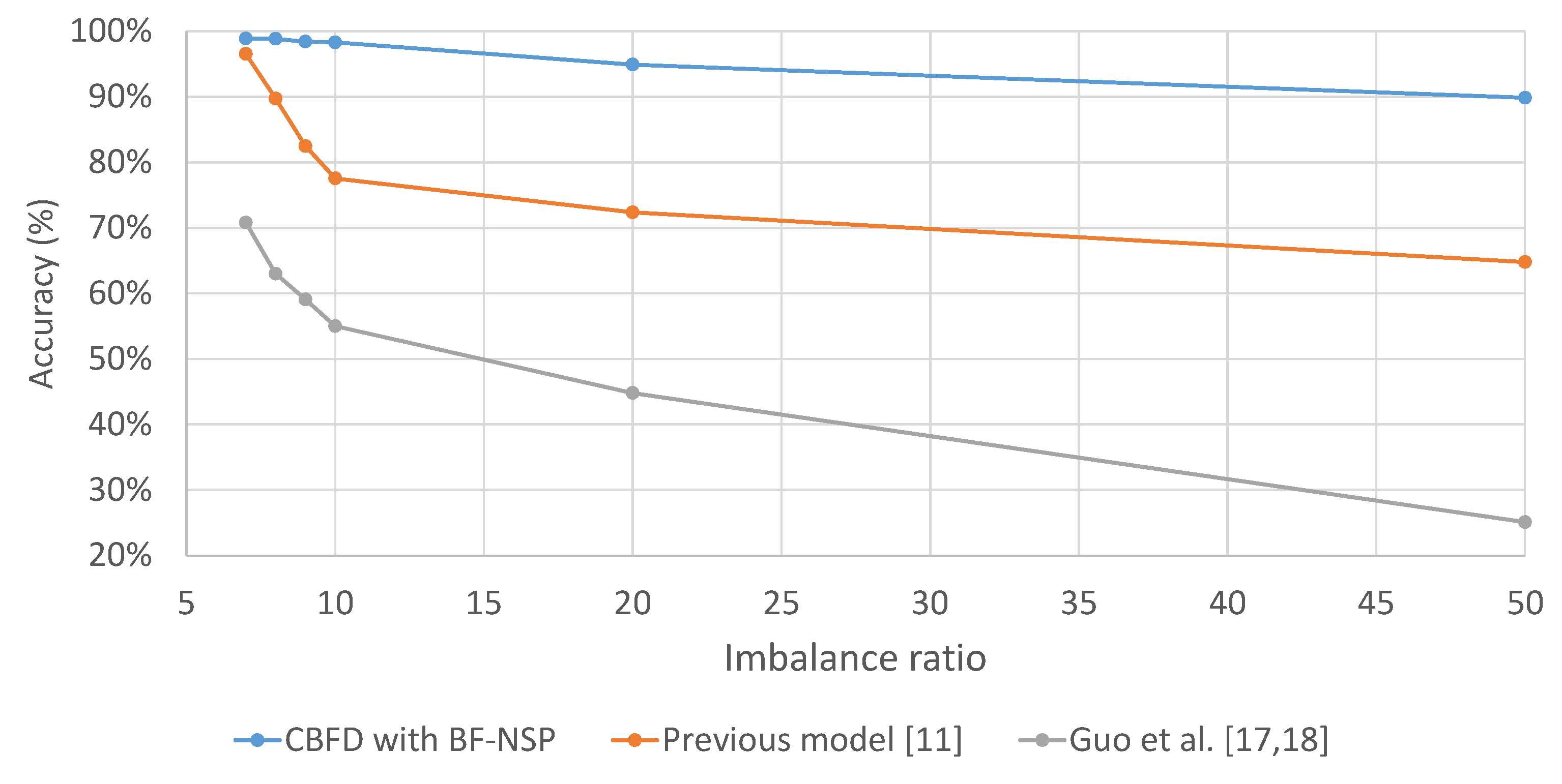
4.2. Testing Classification under Data Imbalanced Conditions

Before evaluating CBFD under data imbalanced condition, we considered two issues: (1) that the data imbalance ratio affects the performance of the classifier more than the number of minority classes; and (2) that the learning rate and epoch number should be considered to prevent over-fitting.

In [11], the degradation of FDD classification accuracy under an unbalanced normal and fault condition ratio was demonstrated; for example,

• False alarms, identified when FDD determines a fault despite normal condition;
• Misfiring, where ground truth observations show a fault condition, but FDD indicates normal condition;
• Confusion, where ground truth observations show one fault condition, but FDD determines another.

According to the previous study [11], the accuracy of testing declines overall when the imbalance ratio of the dataset increased in the case of binary classification (normal or rotor fault/bearing fault). This means that the classification performance of these diagnosis methods was easily affected by the imbalance setting. For motor fault detection, which usually presents severely imbalanced data, misfiring and confusion from the classifier were more important than false alarms.

In addition to increased classifier errors, the over-fitting phenomenon also resulted in poor accuracy for the test dataset, but good accuracy at the training stage. In the learning process, the adaptive moment estimation (Adam) optimizer was employed and tested using static and decaying learning rates. The static learning rate was 0.0001 and the decaying learning rate was set as exponential decay from 0.0005 with 50% decay every 100 epochs (with a total of five decay steps in 500 epochs). The decaying learning rate performed better than the static learning rate, and the accuracy evolution of CBFD became weak at approximately 200 epochs. Therefore, for all further experiments, we determined hyper parameters, with the learning rate and terminal epochs being 50% decay from 0.0005 and 250 epochs, respectively.

To verify the relationship between classification accuracy and data imbalance conditions, we performed two types of experiments: (1) training a model by fixing the number of normal data images to 20,000, which was close to the maximum size of the normal dataset shown in Table 1, and changing the ratio of the data imbalance from 30:1 to 1000:1; (2) fixing the number of normal data images to 10,000 and changing the ratio of data imbalance from 20:1 to 400:1. As the volume of normal data was larger than the volume of fault data, the number of normal data images was fixed and the ratio of data imbalance was changed.

The test set for all conditions contained 300 randomly selected images for each category. To ensure robust results, we took the mean value of 10 trials for each data imbalance rate case as the final result.

In the first experiment, the model was trained by fixing the number of normal data images to 20,000 and changing the ratio of the data imbalance. Figure 8a–c show the overall FDD accuracy and the numbers of misfirings and confusion for various imbalance ratios. No false alarms were observed, but the accuracy is declined and the numbers of misfirings and confusion are increased as the imbalance of the dataset becomes severe. However, the accuracy was still higher than 80%, even when the imbalance ratio was 1000:1.

Figure 8d–f show the result of the second experiment, in which we used 10,000 normal data images. Compared to the first experimental result, it indicates that the numbers of misfirings and confusion were higher for the same imbalance ratio in Figure 8a–c. The accuracy also decreased in general owing to the smaller dataset but still achieved around 80% even for the most severe imbalance ratio of 400:1.

As shown in Figure 9, the proposed method (CBFD with BF-NSP) gave higher classification accuracy than CNN with the continuous wavelet transform scalogram (CWTS) [17,18] and DNN with HHT [11], in which features were extracted using the HHT and the DNN was used as a classifier. To ensure a fair comparison, both models were trained using 5000 random sample data points and tested using 1200 random samples. The comparison results represent the mean values of 10 trials for every data imbalance rate. We found that CBFD with BF-NSP had 95% accuracy, even when the imbalance ratio was 20:1. Its accuracy fell below 90% when the imbalance ratio reached 50:1. On the other hand, the DNN with HHT [11] was more sensitive to the imbalance ratio. Only for an imbalance ratio of 7:1 was the accuracy over 95%. When the imbalance ratio was 9:1, the accuracy was below 80%. In the case of the CNN with CWTS [17,18], the accuracies in the imbalanced conditions were at least 28.1% points lower than CBFD with BF-NSP. When the image transformation using CWTS was applied to the data, the training accuracy of the CNN with CWTS was lower than 90%, so that the results of the CNN with CWTS declined in the data imbalanced conditions. Even though we tried to classify the CWTS images using our CBFD, the differences between the results of the two methods were minor. As shown in

Table 3. Computational time comparison of the convolutional neural network (CNN)-based bearing fault detector (CBFD) with the bearing fault-nested scatter plot (BF-NSP) with other methods.

	Training Time (s)	Testing Time (ms)
CBFD with BF-NSP	805.48	2.59
DNN with HHT	207.50	1.30
CNN with CWTS	66.15	0.38

, the CNN with CWTS provided the fastest training and testing among the three methods because the size of the CWTS image (80 × 80) was smaller than the size of the NSP image (128 × 128). In summary, our CBFD with BF-NSP outperformed the DNN with HHT and the CNN with CWTS, and was capable of detecting bearing faults even when the data imbalance was high.

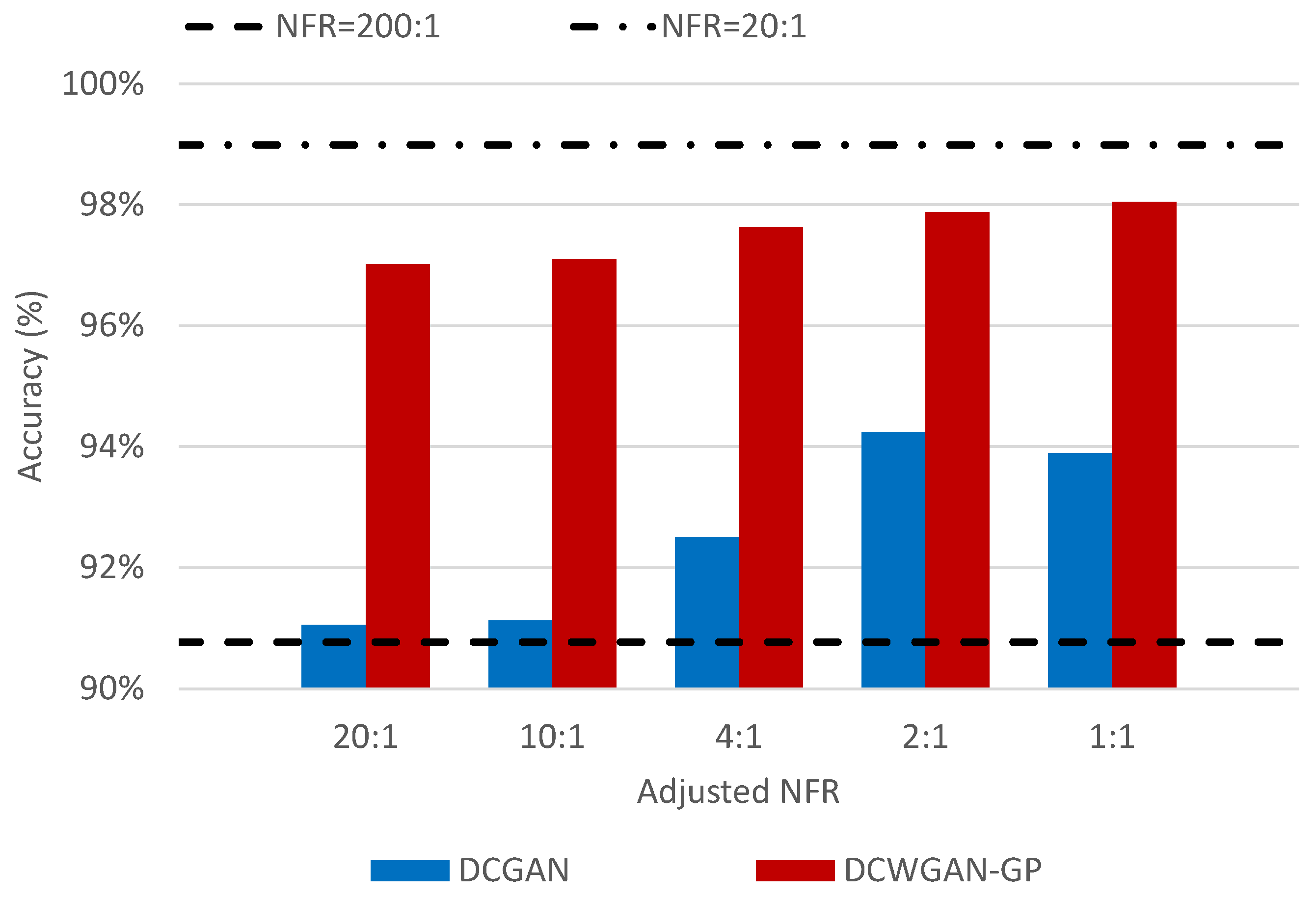
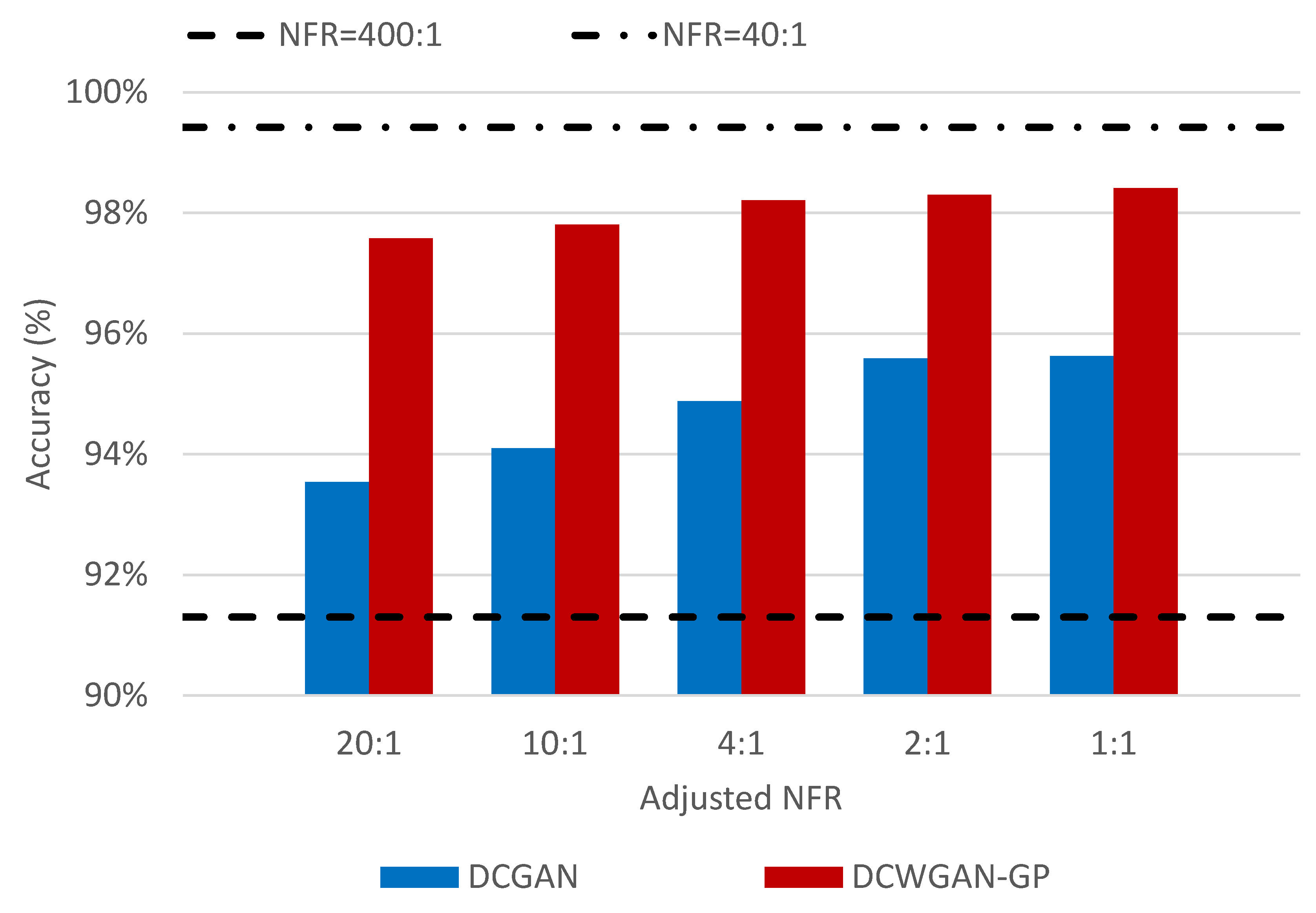
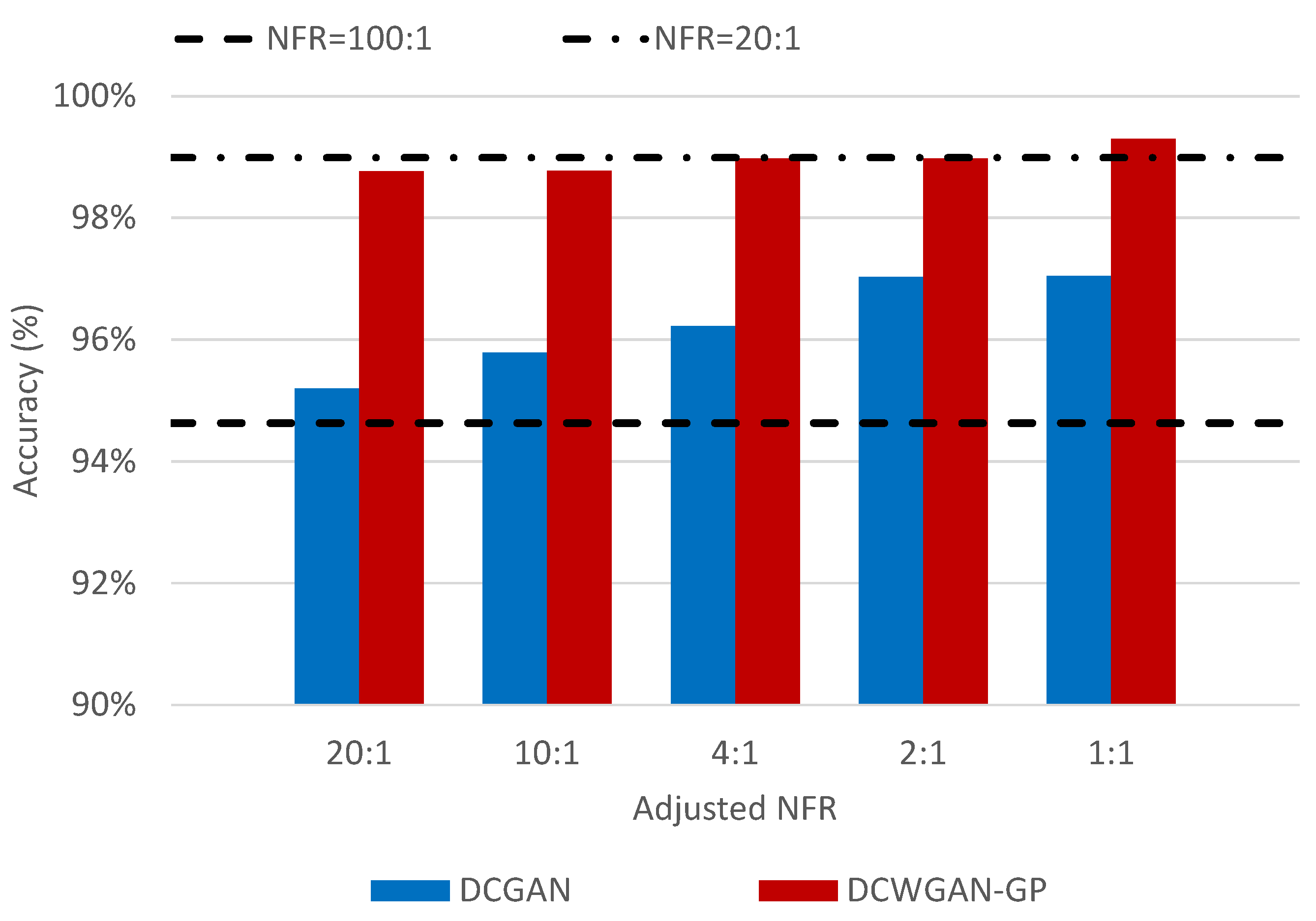
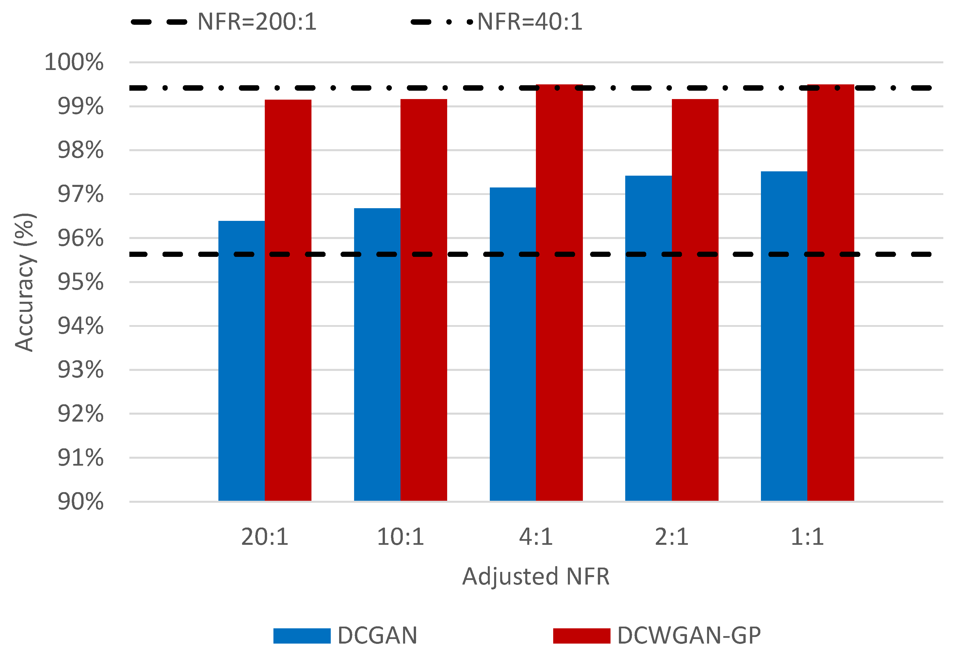
4.3. Testing Classification with Oversampling

We employed oversampling using DCWGAN-GP to improve the classification accuracy under data imbalance conditions. To mitigate problems caused by severe data imbalance, we trained the DCGAN and the proposed DCWGAN-GP for each fault type, allowing the model to generate synthetic fault images. Each model was trained using the available fault dataset defined in Table 1. Figure 10 shows images computed by DCWGAN-GP for each fault type. The generated images can be distinguished by comparison with normal images, and were similar to the images of real bearing fault data. For comparison, images generated using DCGAN [27] are shown in Figure 11; these images can also be distinguished by comparing with normal images and are similar to real bearing fault images.

The images generated using DCGAN contained background noise. To identify the reason for the noise, we monitored the trend of the loss value in the training step (Figure 12). We found that the loss of the DCGAN generator increased as the step proceeded, and that the loss showed significant variation. Figure 13 shows the losses of the proposed DCWGAN-GP; the losses for both the discriminator and the generator converged toward zero as the training step proceeded. Both models were successfully trained for the fault types, however, the objective function of the WGAN-GP provided superior stability and quality of gradients.

We oversampled the fault data of the proposed generative model under various data-imbalanced conditions. Here, the ratio between normal and fault data images is denoted as normal-to-fault ratio (NFR), and the ratio that enhances NFR using oversampling as adjusted NFR (A-NFR).

• NFR = (# of normal data images): (# of fault data images),
• A-NFR = (# of normal data images): (# of fault data images) + (# of oversampled fault data images).

We considered the serious data-imbalanced conditions where NFR > 100:1. In the experiment, not only imbalance ratio, but also the number of samples was considered, because the number of majority and minority datasets had an effect on model training. Firstly, we fixed the number of normal data images to 10,000. Under the condition, we considered two cases of the data-imbalanced condition: fault data images of 50 (which yields NFR = 200:1), and fault data images of 100 (which yield NFR = 100:1). Based on these conditions, we oversampled fault data images using DCGAN and DCWGAN-GP until the number of total fault data images (original and oversampled) reached 500, 1000, 2500, 5000, and 10,000 (which yielded A-NFR = 20:1, 10:1, 5:1, 2:1, and 1:1, respectively). The experimental results of the 10,000 normal data images are shown in Figure 14 and Figure 15. The lower bound of FDD accuracy is 90.77% and 94.63% when NFR is 200:1 and 100:1 without oversampling, respectively. The upper bound of FDD accuracy was 98.99% when NFR was 20:1 without oversampling.

Secondly, we fixed the number of normal data to 20,000. Similar to normal data images of 10,000, we considered two data-imbalanced conditions: NFR = 400:1 and 200:1, and oversampling using DCGAN and DCWGAN-GP was conducted in the cases of A-NFR = 20:1, 10:1, 5:1, 2:1, and 1:1. The experimental results of 10,000 normal data images are shown in Figure 16 and Figure 17. The lower bound of FDD accuracy is 91.30% and 95.63% when NFR is 400:1 and 200:1 without oversampling. The upper bound of FDD accuracy is 99.42% when NFR is 40:1 without oversampling. (The detailed experimental values are shown in

Table 4. Accuracy of original data and oversampled data using the deep convolution generative adversarial network (DCGAN) and the proposed Wasserstein generative adversarial networks with gradient penalty (WGAN-GP) on DCGAN architecture model (DCWGAN-GP) method. (a) Normal- to-fault ratio (NFR) = 200:1 with 10,000 normal data; lower bound = $90.77\%$ at NFR = 200:1, upper bound = $98.99\%$ at NFR = 20:1. (b) NFR = 100:1 with 10,000 normal data; lower bound = $94.63\%$ at NFR = 100:1, upper bound = $98.99\%$ at NFR = 20:1. (c) NFR = 400:1 with 20,000 normal data; lower bound = $91.30\%$ at NFR = 400:1, upper bound = $99.42\%$ at NFR = 40:1. (d) NFR = 200:1 with 20,000 normal data; lower bound = $95.63\%$ at NFR = 200:1, upper bound = $99.42\%$ at NFR = 40:1.

		A-NFR
		20:1	10:1	4:1	2:1	1:1
DCGAN	(a)	91.05%	91.13%	92.51%	94.24%	93.89%
	(b)	95.20%	95.79%	96.23%	97.03%	97.05%
	(c)	93.54%	94.10%	94.88%	95.59%	95.63%
	(d)	96.39%	96.68%	97.15%	97.42%	97.52%
DCWGAN-GP	(a)	97.02%	97.10%	97.63%	97.88%	98.05%
	(b)	98.77%	98.78%	98.98%	98.98%	99.30%
	(c)	97.58%	97.81%	98.21%	98.30%	98.41%
	(d)	99.15%	99.16%	99.50%	99.16%	99.50%

.)

Oversampling using DCWGAN-GP and DCGAN improved the FDD overall accuracy. In the case of 10,000 normal data images (shown in Figure 14 and Figure 15), DCWGAN-GP improved the accuracy by 7.28% points and 4.67% points at A-NFR = 1:1 compared to the accuracy at NFR = 200:1 and 100:1. DCGAN also improved the accuracy by 3.12% points and 2.42% points at A-NFR = 1:1 compared to the accuracy at NFR = 200:1 and 100:1. Similarly, oversampling using DCWGAN-GP and DCGAN showed better accuracy compared to the base lines that were no sampling cases (shown in Figure 16 and Figure 17).

DCWGAN-GP outperformed DCGAN in generative oversampling. In the case of NFR = 100:1 (shown in Figure 15), DCWGAN-GP improved accuracy from 4.1 to 4.7% points compared to no oversampling when DCGAN did only from 0.5 to 2.4% points. In addition, in the case of NFR = 400:1 (shown in Figure 16), oversampling using DCWGAN-GP improved the accuracy by 6.28 to 7.11% points when the result of DCGAN was only 2.24 to 4.33% points. Furthermore, the variance in accuracy with oversampling of DCWGAN-GP was around 1%, with overall accuracies 98% and 99% higher, respectively. While the accuracy for oversampling was lower than just 2% or less than the accuracy for upper bound results ($NFR=$ 20:1 and 40:1, in the case of normal data images 10,000 and 20,000, respectively.)

As seen in Figure 14, Figure 15, Figure 16 and Figure 17, as oversampling enhanced A-NFR, the accuracy increased. We emphasize here that oversampling using DCWGAN-GP showed 97% or higher accuracy when A-NFR was 20:1. As mentioned before, BF-NSP and CBFD showed good performance in the tolerable imbalance condition such as NFR = 20:1 to 50:1. This means that oversampling using DCWGAN until A-NFR met the tolerable imbalance conditions was enough for FDD accuracy. DCGAN showed less than 96.5% accuracy (gap between DCWGAN-GP and DCGAN ranges from 2.7 to 5.97% points) when A-NFR is 20:1. Therefore, DCGAN required more oversampling data than DCWGAN-GP, and this fact resulted in the increased cost of computation.

NFR was one of the reasons for FDD performance degradation, but the number of datasets was also important. Figure 14 and Figure 17 have the same NFR = 200:1, but different number of datasets. Comparing these two results, the case of 20,000 normal data images showed better accuracy than the case of 10,000 normal data images.

5. Conclusions

In this study, we developed a novel generative oversampling method to address the data imbalance issue for bearing FDD. In short, because the volume of faulty condition data is much lower than that of normal condition data, a lower recognition accuracy of the fault condition results. Before introducing the oversampling method, the proposed method was used to transform time-series data into the image domain via the NSP method; bearing faults in the induction motor were classified using designed CNNs. The classification accuracy was 2.4 to 25% points higher than that of previous work; furthermore, our approach provided around 90% accuracy even when the imbalance ratio was weak (50:1); the accuracy declined to 80% when the imbalance ratio increased to 1000:1. To overcome the data imbalance problem, we generated fault images using DCWGAN-GP. Experiments demonstrated that the proposed method improves accuracy by 7.2 and 4.27% points on average and gives maximum values with 5.97 and 3.57% points higher accuracy than the previously developed DCGAN approach. Additionally, the accuracy of the proposed method was close to that under data imbalance ratio conditions of 20:1 and 40:1 without oversampling.

As future work, we will consider accuracy improvement in generative oversampling methods. Even though the proposed DCWGAN-GP improved the FDD accuracy in the given imbalanced data conditions, there is less than a 2% gap compared to the weak imbalanced data conditions. Furthermore, comparing to the DNN with HHT [11] and the CNN with CWTS [17,18], CBFD with BF-NSP takes at least twice training and testing time. We will optimize the classification network and reduce computational time. In addition, we plan to apply the proposed methods to other data-imbalanced conditions in FDD.

References

1. Baptista, M.; Sankararaman, S.; de Medeiros, I.P.; Nascimento, C., Jr.; Prendinger, H.; Henriques, E.M. Forecasting fault events for predictive maintenance using data-driven techniques and ARMA modeling. Comput. Ind. Eng. 2018, 115, 41–53. [Google Scholar] [CrossRef]
2. Benbouzid, M.E.H.; Kliman, G.B. What stator current processing-based technique to use for induction motor rotor faults diagnosis? IEEE Trans. Energy Convers. 2003, 18, 238–244. [Google Scholar] [CrossRef]
3. Antonino-Daviu, J.A.; Riera-Guasp, M.; Pineda-Sanchez, M.; Pérez, R.B. A critical comparison between DWT and Hilbert–Huang-based methods for the diagnosis of rotor bar failures in induction machines. IEEE Trans. Ind. Appl. 2009, 45, 1794–1803. [Google Scholar] [CrossRef]
4. Nandi, S.; Toliyat, H.A.; Li, X. Condition monitoring and fault diagnosis of electrical motors—A review. IEEE Trans. Energy Convers. 2005, 20, 719–729. [Google Scholar] [CrossRef]
5. Zhang, P.; Du, Y.; Habetler, T.G.; Lu, B. A survey of condition monitoring and protection methods for medium-voltage induction motors. IEEE Trans. Ind. Appl 2011, 47, 34–46. [Google Scholar] [CrossRef]
6. Zhang, B.; Sconyers, C.; Byington, C.; Patrick, R.; Orchard, M.E.; Vachtsevanos, G. A probabilistic fault detection approach: Application to bearing fault detection. IEEE Trans. Ind. Electron. 2011, 58, 2011–2018. [Google Scholar] [CrossRef]
7. Deng, F.; Guo, S.; Zhou, R.; Chen, J. Sensor multifault diagnosis with improved support vector machines. IEEE Trans. Autom. Sci. Eng. 2017, 14, 1053–1063. [Google Scholar] [CrossRef]
8. Gu, X.; Deng, F.; Gao, X.; Zhou, R. An Improved Sensor Fault Diagnosis Scheme Based on TA-LSSVM and ECOC-SVM. J. Syst. Sci. Complex. 2018, 31, 372–384. [Google Scholar] [CrossRef]
9. Li, C.; de Oliveira, J.L.V.; Lozada, M.C.; Cabrera, D.; Sanchez, V.; Zurita, G. A systematic review of fuzzy formalisms for bearing fault diagnosis. IEEE Trans. Fuzzy Syst. 2018. [Google Scholar] [CrossRef]
10. Esfahani, E.T.; Wang, S.; Sundararajan, V. Multisensor wireless system for eccentricity and bearing fault detection in induction motors. IEEE/ASME Trans. Mech. 2014, 19, 818–826. [Google Scholar] [CrossRef]
11. Lee, Y.O.; Jo, J.; Hwang, J. Application of deep neural network and generative adversarial network to industrial maintenance: A case study of induction motor fault detection. In Proceedings of the 2017 IEEE International Conference on Big Data (Big Data), Boston, MA, USA, 11–14 December 2017; pp. 3248–3253. [Google Scholar]
12. Chen, Z.; Li, W. Multisensor feature fusion for bearing fault diagnosis using sparse autoencoder and deep belief network. IEEE Trans. Instrum. Meas. 2017, 66, 1693–1702. [Google Scholar] [CrossRef]
13. Qin, Y.; Wang, X.; Zou, J. The Optimized Deep Belief Networks With Improved Logistic Sigmoid Units and Their Application in Fault Diagnosis for Planetary Gearboxes of Wind Turbines. IEEE Trans. Ind. Electron. 2019, 66, 3814–3824. [Google Scholar] [CrossRef]
14. Zhao, G.; Liu, X.; Zhang, B.; Zhang, G.; Niu, G.; Hu, C. Bearing Health Condition Prediction Using Deep Belief Network. In Proceedings of the Annual Conference of Prognostics and Health Management Society, Orlando, FL, USA, 15–18 April 2017; pp. 2–5. [Google Scholar]
15. Tang, S.; Shen, C.; Wang, D.; Li, S.; Huang, W.; Zhu, Z. Adaptive deep feature learning network with Nesterov momentum and its application to rotating machinery fault diagnosis. Neurocomputing 2018, 305, 1–14. [Google Scholar] [CrossRef]
16. Oh, H.; Jung, J.H.; Jeon, B.C.; Youn, B.D. Scalable and Unsupervised Feature Engineering Using Vibration-Imaging and Deep Learning for Rotor System Diagnosis. IEEE Trans. Ind. Electron. 2018, 65, 3539–3549. [Google Scholar] [CrossRef]
17. Guo, S.; Yang, T.; Gao, W.; Zhang, C. A Novel Fault Diagnosis Method for Rotating Machinery Based on a Convolutional Neural Network. Sensors 2018, 18, 1429. [Google Scholar] [CrossRef] [PubMed]
18. Guo, S.; Yang, T.; Gao, W.; Zhang, C.; Zhang, Y. An intelligent fault diagnosis method for bearings with variable rotating speed based on Pythagorean spatial pyramid pooling CNN. Sensors 2018, 18, 3857. [Google Scholar] [CrossRef] [PubMed]
19. Wang, S.; Xiang, J.; Zhong, Y.; Zhou, Y. Convolutional neural network-based hidden Markov models for rolling element bearing fault identification. Knowl.-Based Syst. 2018, 144, 65–76. [Google Scholar] [CrossRef]
20. LIU, T.; LI, G. The imbalanced data problem in the fault diagnosis of rolling bearing. Comput. Eng. Sci. 2010, 32, 150–153. [Google Scholar]
21. Ramentol, E.; Caballero, Y.; Bello, R.; Herrera, F. SMOTE-RSB*: A hybrid preprocessing approach based on oversampling and undersampling for high imbalanced data-sets using SMOTE and rough sets theory. Knowl. Inf. Syst. 2012, 33, 245–265. [Google Scholar] [CrossRef]
22. Ng, W.W.; Hu, J.; Yeung, D.S.; Yin, S.; Roli, F. Diversified sensitivity-based undersampling for imbalance classification problems. IEEE Trans. Cybern. 2015, 45, 2402–2412. [Google Scholar] [CrossRef]
23. Lu, X.; Chen, M.; Wu, J.; Chan, P. A Feature-Partition and Under-Sampling Based Ensemble Classifier for Web Spam Detection. Int. J. Mach. Learn. Comput. 2015, 5, 454. [Google Scholar] [CrossRef]
24. Buda, M.; Maki, A.; Mazurowski, M.A. A systematic study of the class imbalance problem in convolutional neural networks. Neural Netw. 2018, 106, 249–259. [Google Scholar] [CrossRef] [PubMed]
25. Jo, J.; Lee, Y.O.; Hwang, J. Multi-layer Nested Scatter Plot—A data wrangling method for correlated multi-channel time series signals. In Proceedings of the 2018 IEEE International Conference on Artificial Intelligence for Industries, Laguna Hills, CA, USA, 26–28 September 2018. [Google Scholar]
26. Gulrajani, I.; Ahmed, F.; Arjovsky, M.; Dumoulin, V.; Courville, A.C. Improved training of wasserstein gans. In Proceedings of the Advances in Neural Information Processing Systems, Long Beach, CA, USA, 4–9 December 2017; pp. 5767–5777. [Google Scholar]
27. Radford, A.; Metz, L.; Chintala, S. Unsupervised representation learning with deep convolutional generative adversarial networks. arXiv, 2015; arXiv:1511.06434. [Google Scholar]
28. Veltman, A.; Pulle, D.W.; De Doncker, R.W. Fundamentals of Electrical Drives; Springer: Cham, Switzerland, 2007. [Google Scholar]
29. McFadden, P.; Smith, J. Vibration monitoring of rolling element bearings by the high-frequency resonance technique–A review. Tribol. Int. 1984, 17, 3–10. [Google Scholar] [CrossRef]
30. Yang, M.; Yin, J.; Ji, G. Classification methods on imbalanced data: A survey. J. Nanjing Normal Univ. 2008, 8, 8–11. [Google Scholar]
31. Goodfellow, I.; Pouget-Abadie, J.; Mirza, M.; Xu, B.; Warde-Farley, D.; Ozair, S.; Courville, A.; Bengio, Y. Generative adversarial nets. In Proceedings of the Advances in Neural Information Processing Systems, Montreal, QC, Canada, 8–13 December 2014; pp. 2672–2680. [Google Scholar]
32. Arjovsky, M.; Chintala, S.; Bottou, L. Wasserstein generative adversarial networks. In Proceedings of the International Conference on Machine Learning, Sydney, NSW, Australia, 6–11 August 2017; pp. 214–223. [Google Scholar]
Figure 1. Test bench and bearings. (a) test bench (model: EMOD FKFIE2100LA, Pmech: 3 kW, nnom: 1440/min, Vnom: 400 V, Inom: 6.4 A, cos ϕ : 0.78), (b) sensors mounted on the motor, (c) bearing with different faulty conditions.
Applsci 09 00746 g001
Figure 2. Bearing fault-nested scatter plot (BF-NSP) process.
Applsci 09 00746 g002
Figure 3. Spectral density difference in resonance bandwidths.
Applsci 09 00746 g003
Figure 4. Convolutional neural network (CNN)-based bearing fault detector (CBFD) architecture.
Applsci 09 00746 g004
Figure 5. Deep convolutional generative adversarial networks (DCGAN) for generative model of BF-NSP images.
Applsci 09 00746 g005
Figure 6. Images of normal data under various conditions.
Applsci 09 00746 g006
Figure 7. Images of bearing fault data. (a) Contaminant, (b) outer high, (c) outer medium, (d) outer low, (e) inner high, and (f) inner medium.
Applsci 09 00746 g007
Figure 8. Test results for fixed normal data at 20,000 and changing ratio of data imbalance: (a) accuracy, (b) misfiring, and (c) confusion. Test results with fixed normal data to 10,000: (d) accuracy, (e) misfiring, and (f) confusion.
Applsci 09 00746 g008
Figure 9. Comparison of CBFD with BF-NSP with other methods.
Applsci 09 00746 g009
Figure 10. Generated images of bearing fault data using the Wasserstein generative adversarial networks with gradient penalty on the DCGAN architecture model (DCWGAN-GP). (a) Contaminant, (b) outer high, (c) outer medium, (d) outer low, (e) inner high, and (f) inner medium.
Applsci 09 00746 g010
Figure 11. Generated images of bearing fault data using the DCGAN. (a) Contaminant, (b) outer high, (c) outer medium, (d) outer low, (e) inner high, and (f) inner medium.
Applsci 09 00746 g011
Figure 12. Losses of the DCGAN [27]. (a) Losses of the discriminator, and (b) losses of the generator.
Applsci 09 00746 g012
Figure 13. Losses of DCWGAN-GP. (a) Losses of the discriminator, and (b) losses of the generator.
Applsci 09 00746 g013
Figure 14. Fault detection and diagnosis (FDD) accuracy testing:normal-to-fault-ratio (NFR) = 200:1 with 10,000 normal data.
Applsci 09 00746 g014
Figure 15. FDD accuracy testing:NFR = 100:1 with 10,000 normal data.
Applsci 09 00746 g015
Figure 16. FDD accuracy testing:NFR = 400:1 with 20,000 normal data.
Applsci 09 00746 g016
Figure 17. FDD accuracy testing:NFR = 200:1 with 20,000 normal data.
Applsci 09 00746 g017