Decision Support Application for Energy Consumption Forecasting

Abstract

Energy consumption forecasting is crucial in current and future power and energy systems. With the increasing penetration of renewable energy sources, with high associated uncertainty due to the dependence on natural conditions (such as wind speed or solar intensity), the need to balance the fluctuation of generation with the flexibility from the consumer side increases considerably. In this way, significant work has been done on the development of energy consumption forecasting methods, able to deal with different forecasting circumstances, e.g., the prediction time horizon, the available data, the frequency of data, or even the quality of data measurements. The main conclusion is that different methods are more suitable for different prediction circumstances, and no method can outperform all others in all situations (no-free-lunch theorem). This paper proposes a novel application, developed in the scope of the SIMOCE project (ANI|P2020 17690), which brings together several of the most relevant forecasting methods in this domain, namely artificial neural networks, support vector machines, and several methods based on fuzzy rule-based systems, with the objective of providing decision support for energy consumption forecasting, regardless of the prediction conditions. For this, the application also includes several data management strategies that enable training of the forecasting methods depending on the available data. Results show that by this application, users are endowed with the means to automatically refine and train different forecasting methods for energy consumption prediction. These methods show different performance levels depending on the prediction conditions, hence, using the proposed approach, users always have access to the most adequate methods in each situation.

1. Introduction

In recent decades, researchers have studied the problem of short-term forecasting energy consumption and its role in energy control systems [1]. These studies prove that an accurate short-term load prediction represents a high potential for electric utility corporations. This importance can be recognized while load estimation is used to control operations decisions such as dispatch, unit commitment, fuel allocation, and maintenance [2,3].

The three main economic sectors with the highest amount of energy consumption are industry, transportation, and buildings, where buildings present the most significant portion [4]. According to recent studies in European Union countries, 40% of the total energy consumption is consumed in buildings [5]. Also, in the USA, the consumed energy by heating, ventilating, and air-conditioning (HVAC) systems in buildings correspond to around 44% of domestic energy consumption [6].

Due to the amount of the energy consumption in buildings, prediction of this consumption is significant to improve the performance of energy systems, have better control on the energy distribution network, and reduce this amount of energy consumption. On the other hand, the energy system in buildings can be quite complex, depending on the types of building and types of energy consumers. Most of the considered building types are office, residential, and engineering buildings, varying from small rooms to big estates [7]. The consumption of a building is mostly divided into lights, HVAC, and electrical sockets; therefore, many different factors must be considered to have a proper recognition of the consumption behavior, such as environmental variables, number of users, etc.

The complexity of energy consumption behavior in buildings makes it difficult to have a forecasting model to predict this behavior with acceptable performance. Many different studies have been published which propose various forecasting algorithms and models to predict the value of energy consumption. This approach can be categorized into statistical, engineering, and artificial intelligence models [4]. In the engineering methods, physical principles are used to calculate thermal dynamics and energy behavior on the whole building level or for sub-level components [7]. To have a good performance from these methods, a piece of high-level information about the structure of the building and different parameters are required, which might not be available. Moreover, to build a model which is based on complex physical principles, a high level of expertise is needed [8].

Statistical models are linear models based on statistical approaches, using historical data to obtain the relationships between data. Clearly, in these models, historical data plays an important role in acquiring a reliable result. Unlike the engineering models, in the statistical models, no physical structure is included [9]. The linear models consist of regression-type models, which are autoregressive (AR), autoregressive with exogenous variable (ARX), moving average (MA), autoregressive moving average (ARMA), autoregressive moving average with exogenous variable (ARMAX), and autoregressive integrated moving average (ARIMA) [10,11,12].

Artificial intelligence models, which are also known as nonlinear statistical models, can be categorized as Artificial Neural Networks (ANN), Support Vector Machines (SVMs), Fuzzy Rule-Based Systems (FRBS), and hybrid approaches [13,14,15]. Recently, these models have been widely used to solve many estimation problems. For example, in the study presented in [8], the author implements a neural network model to forecast the electricity demand of a bioclimatic building, located in the south-east of Spain. The results of this work show that this model can predict this value by an error of 11.48%. In [16], ANN is used to predict a day-ahead energy consumption profile for an office building. This work divides the total energy consumption of the building into three values, which present the consumption of lights, HVAC, and electrical sockets. For each one of these three consumers, a specific forecasting model is created using external facility data, such as temperature and humidity. The results prove that this approach predicts the total energy consumption by an error of 13.6%. Many fuzzy rule-based methods have been purposed to be used in various forecasting proposes. 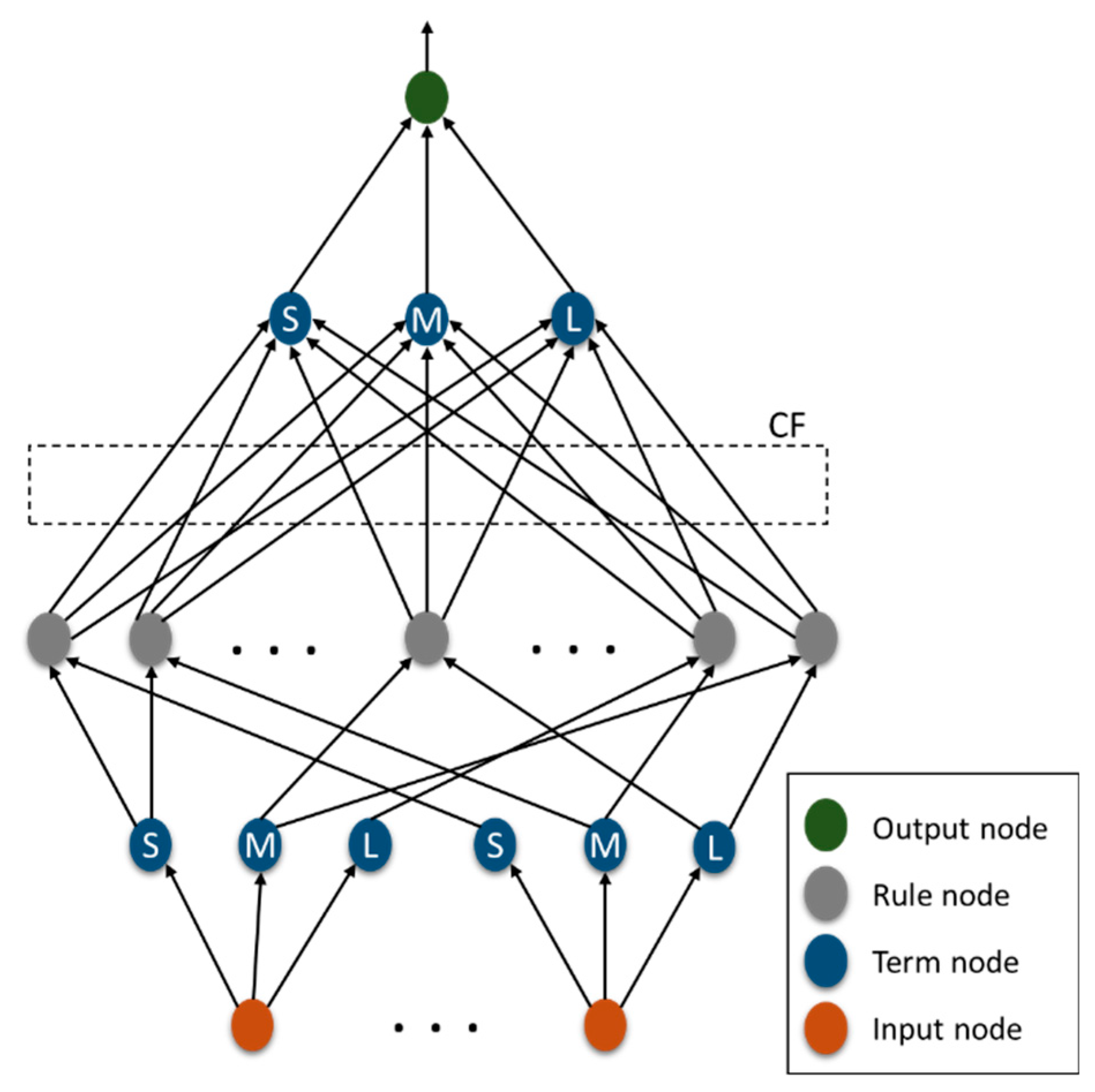In [17], five fuzzy rule-based methods, namely as Wang and Mendel’s method (WM), Hybrid neural Fuzzy Inference System (HyFIS), Genetic fuzzy systems for fuzzy rule learning based on the MOGUL methodology (GFS.FR.MOGUL), Genetic lateral tuning and rule selection of linguistic fuzzy systems (GFS.LT.RS), and the simplified TSK fuzzy rule-generation method using heuristics and gradient descent method (FS.HGD), are used to predict the hourly energy consumption of TRT-France buildings located in Paris, France. This study shows that in this case, the GFS.FR.MOGUL presents the most trustable results, followed by HyFIS and WM. In [18], a hybrid probabilistic fuzzy ARIMA model is presented, which is used to obtain a consumption forecasting in commodity markets. This hybrid model offers a combination of artificial intelligence models with linear statistical models where computational intelligence tools are used as well as soft computing techniques. The work presented in [19] proposes a model to forecast the energy consumption of public buildings to improve energy saving; Elman neural networks are used to make this prediction. Artificial intelligence models also can be used in other situation of forecasting. For example [20], a study has been presented that uses SVM to estimate the short-term wind speed where the results are also compared to the results of several ANN-based approaches. More studies using these forecasting approaches to solve different prediction and estimation problems can be found in [21,22,23].

Energy consumption estimation has an essential role in energy system management and the energy distribution network. However, to implement the forecasting models a high knowledge about programming languages, data storage systems, and data preparation is required. This fact can be a limitation for users working in this industry, which do not have this knowledge. In this way, this work proposes an application that makes it possible for the user to use different forecasting algorithms to predict the energy consumption of buildings. The proposed application, developed in the scope of the SIMOCE project (ANI|P2020 17690), is meant to be used by users who do not have enough knowledge to implement these methods and run the models on their own. Five forecasting methods are considered in this application, namely ANN, SVM, and three FRBS methods including, HyFIS, WM, and GFS.FR.MOGUL. Additionally, four different strategies to manage and prepare the data sets to train the methods are included. In this way, the users have access to several of the most relevant forecasting methods in this domain, as well as different approaches for data treatment and training. Besides facilitating the forecasting process for users with no experience in machine learning, the proposed application also enables mitigating the difficulties in choosing the best approaches for each prediction circumstance (amount of data, available data variables), as it provides the means to reach results with the different algorithms, and thus supports the user decisions in selecting the most suitable solution for each situation. In addition to the abovementioned benefits, which are mostly directed to users in the power and energy domain, the presented application also has direct advantages in multiple other domains, e.g., as facilitator for the implementation of energy management methods in manufacturing systems. By helping to reach suitable forecasts of energy consumption, the proposed application may be directly integrated with switch-off energy saving methods for production lines, such as the model proposed in [24]; or even integrated in advanced optimization methods for energy saving, as presented in [25]. Moreover, by being developed as a domain-agnostic application, it can be applied and used in multiple other application domains for forecasting purposes, simply needing access to the log of historic data.

After this introductory section, Section 2 presents the proposed model, including the description of the considered forecasting methods, data management strategies, and the architecture of the application. Section 3 presents a case study that shows the performance of the proposed application using real consumption data and compares the results achieved by the different forecasting methods under distinct prediction circumstances. Finally, Section 4 presents and discusses the most relevant conclusions of this work.

2. Material and Methods

This work presents a Java-based software application that provides the user with the means to predict the energy consumption in buildings for the following hours, using five different forecasting methods. This section includes the description of the forecasting methods and the applied data in this software.

2.1. Forecasting Methods

This software currently integrates five forecasting methods based on different approaches to predict a more reliable value for energy consumption. These methods are, ANN, SVM, and three FRBS methods including, HyFIS, Wang and Mendel’s Fuzzy Rule Learning Method (WM), Genetic Fuzzy Systems for Fuzzy Rule learning based on the MOGUL methodology (GFS.FR.MOGUL). The following sub-sections describe the implementation of these methods.

2.1.1. ANN

ANN are widely used to solve many forecasting problems and are the most common methods for energy consumption forecasting. The main reason for their success is that the provided solution to model complex nonlinear relationships by these models is much better than the solutions of the other traditional linear models [26]. Several studies have been published using this method to predict the energy consumption for different terms and different situations of consumption. This method is inspired by the human brain and its number of neurons with high interconnectivity. ANNs are several combined nodes or neurons, divided into different levels and interconnected by numeric weights. They resemble the human brain in two fundamental points: the knowledge being acquired from the surrounding environment, through a learning process; and the network’s nodes being interconnected by weights (synaptic weights), used to store the knowledge. Each neuron executes a simple operation, the weighted sum of its input connections, which originates the exit signal that is sent to the other neurons. The network learns by tuning the connection weights to produce the desired output [27]. Based on many correct examples ANNs can change their connection weights until they generate outputs that are coincident with the correct values. This way, the ANN can extract basic rules from data [13].

2.1.2. SVM

The first algorithm for pattern recognition was created by R. A. Fisher in 1963 [27]. The first running kernel of SVM was designed in the sequence of [27] by Vapnik, implementing a generalization of the nonlinear algorithm Generalized Portrait and only for classification and linear problems. Furthermore, in 1979, the statistical learning theory was developed by Vapnik. However, the current form of the SVM approach was presented with a paper at the COLT conference, in 1992 [14]. The structure of the data to be used in an SVM must follow the format suggested in Equation (1).

$$\left(y_1,x_1\right),\dots ,\left(y_i,x_i\right), x\in R^n, y\in R$$

(1)

Where each example x_i is a space vector example; y_i has a corresponding value; n is the size of training data. For classification: y_i assumes finite values; in binary classifications: y_i ∈ {+1,−1}; in digit recognition: y_i ∈ {1,2,3,4,5,6,7,8,9,0}; and for regression purposes, y_i is a real number (y_i ∈ R). The implementation of SVM requires considering some important aspects, namely:

• Feature Space
• Loss Functions
• Kernel Functions

The most applicable kernels for time series forecasting, as in the problem considered in this work, are the Radial Basis Function (RBF) and the exponential Radial Basis Function (eRBF) [28]. These two kernels are specifically directed to regression in time series data. The SVM approach takes as parameters:

• training Limit—limit number of training data;
• kernel—kernel that is used in the regression process;
• ε-insensitive—the error that is permitted, i.e., the lower the value, the higher the exigency of the regression process;
• limit—limit of the kernel function;
• σ—the angle of the kernel function;
• offset—offset of the kernel function.

A suitable combination of these parameters is essential to achieve quality results. The most suitable combination is highly dependable on the characteristics and particularities of each distinct problem. Therefore, an exhaustive sensitivity analysis must be performed for each application, to achieve conclusions on the best combinations of parameters that should be used.

2.1.3. FRBS

Fuzzy logic has been proposed by Zadeh in 1965 [15], and it represents the reasoning of human experts in production rules (a set of IF-THEN rules) to handle real-life problems from domains such as control, prediction, and inference, data mining, bioinformatics data processing, robotics, and speech recognition. FRBSs are the combination of the fuzzy logic and the other data mining techniques which are also known as fuzzy inference systems and fuzzy models [29]. An alternative and effective way to extract the required information in the right format from human experts is to gain the knowledge by generating the fuzzy IF-THEN rules automatically from the numerical training data. While modeling an FRBS, structure identification and parameter estimation must be considered as two essential process where the structure identification is a process to find appropriate fuzzy IF-THEN rules and to determine the overall number of rules, and parameter estimation is applied to tune parameters of membership functions. The FRBSs are the combination of fuzzy logic and other techniques.

This work takes advantage of using the FRBS package [29] to implement fuzzy rule-based forecasting methods. The package divides these forecasting methods into five groups based on the used techniques in their implementation. These groups are:

(1)

FRBS based on space partition

(2)

FRBS based on neural networks

(3)

FRBS based on clustering approaches

(4)

FRBS based on genetic algorithms

(5)

FRBS based on the gradient descent method

Three FRBS forecasting methods have been chosen to be used in this work. Following sections explain the structure of these methods.

A. HyFIS

HyFIS was proposed by Kim and Kasabov [30], and it is a combination of fuzzy logic with neural networks. As Figure 1 presents, the learning process of this method is based on two phases. The first phase is the structure learning, where the method uses the knowledge acquisition module to find and create the rules. The second phase membership functions will be tuned to achieve a desired level of performance, which is the parameter learning phase.

When a new set of data is inserted into the method, a new rule will be created for the new data, and the fuzzy rule base gets updated. Having an easy updatable fuzzy rule base can be named as one of the advantages of this approach [31].

The neuro-fuzzy model in the HyFIS is a combination of fuzzy systems and a multilayer ANN. As Figure 2 shows, this structure contains five layers, where the input state and output control/decision signals, respectively. Also, the nodes in the hidden layers represent the membership functions and rules.

The nodes in the first layer represent the inputs of the method. The nodes in the second and fourth layer, act as the Membership Functions (MF) to express the input-output fuzzy linguistic variables. The fuzzy sets in these layers are presented as large (L), medium (M), and small (S). However, in some cases, this distribution can be more specific and be shown as large positive (LP), small positive (SP), zero (ZE), small negative (SN), and large negative (LN). The third layer includes the rule nodes, every node in this layer is a fuzzy rule. The connection weights between the third and fourth layer represent certainty factors (CFs) of the associated rules, i.e., each rule is activated to a certain degree controlled by the weight values. In the end, the nodes in the fifth layer present the outputs of the system.

B. WM

The Wang and Mendel’s method has been known as a simple method with an acceptable performance [32]. The implementation of fuzzy rules in this method is based on four steps which are presented in Figure 3.

In the first step, the input and output spaces of the given data are equally divided into fuzzy regions which can be obtained from the expert information or by a normalization process. In the second phase, the fuzzy rules will be created by using the database from the first phase. First, it calculates the degrees of the membership functions for every value in the training data. Then, a linguistic term with a maximum degree in each variable will be determined. The degrees for each rule are determined in the third step by aggregating the degree of membership functions in the antecedent and consequent parts. $I F x1 is A1 and \dots and xn is An THEN y is B$, be the linguistic rule generated from the example $el$, $l$ = 1,…,. The importance degree associated with it will be obtained as Equation (2) [33]:

$$G\left(R_l\right)=\mu A_1\left(x_1^l\right), \dots , \mu A_1\left(x_n^l\right).\mu B\left(y^l\right)$$

(2)

Finally, in the fourth step, the candidate rules will be divided into different groups, where, each group is composed of all the candidate rules with the same antecedent.

C. Genetic fuzzy systems for fuzzy rule learning based on the MOGUL methodology (GFS.FR.MOGUL)

GFS.FR.MOGUL forecasting methods have been proposed by Herrera et al. in 1995 [34]. This method implements a Genetic Algorithm (GA) determining the structure of the fuzzy IF-THEN rules and the membership function parameters. This method considers two types of IF-THEN rules.

• Descriptive rules
• Approximate/free semantic approaches

In the first type, the linguistic labels illustrate a real-world semantic, and the linguistic labels are uniformly defined for all rules. In contrast, in the approximate approach, there is any associated linguistic label.

To obtain an acceptable performance from Fuzzy Rule-Based Systems different statistical properties have to be considered [35]. In the Generated Fuzzy Rule Bases (GFRB) obtained from MOGUL, two statistical properties will be considered, which are:

• completeness
• consistency

As an inductive approach to building GFRBSs is considered, both properties will be based on the existence of a training data set, Ep, composed of numerical input-output problem variable pairs. In the field of inductive learning τ-completeness means that the system should be able to infer a proper output for all possible system input [36]. Expressions (3)–(5), present this property mathematically formulated:

$$C_R\left(e_l\right)={\displaystyle \bigcup }_{i=1\dots t}{R}_i\left(e_l\right)\ge \tau , l=1,\dots ,p$$

(3)

$$\left[R_i\left(e_l\right)=\ast \left(A_i\left(e{x}^l\right),B_i\left(e{y}^l\right)\right)\right]$$

(4)

$$A_i\left(e{x}^l\right)=\ast \left(A_{i1}\left(e{x}_1^l\right),\dots ,A_{in}\left(e{x}_n^l\right)\right)$$

(5)

where * is a t-norm, and $R_i$($e_l$) is the compatibility degree between the rule R_i and the example $e_l$.

For the Consistency of a FRBS, a generic set of IF-THEN rules is considered while it does not contain contradictions. It is necessary to relax the consistency property to consider the fuzzy rule bases, and it will be done by means of the positive and negative examples of concepts. Following equations present the examples of the positive and negative set for the rule $R_i$.

• Positive:

  $$E^{+}\left(R_i\right)=\left\{e_l\in \frac{E_p}{R_i\left(e_l\right)}\ge 0\right\}$$

  (6)
• Negative:

  $$E^{-}\left(R_i\right)=\left\{e_l\in \frac{E_p}{R_i\left(e_l\right)}=0 and A_i\left(e{x}^l\right)>0\right\}$$

  (7)

And by giving the value and Equations (8) and (9):

$$n_{R_i}^{+}=\left|E^{+}\left(R_i\right)\right|$$

(8)

$$n_{R_i}^{-}=\left|E^{-}\left(R_i\right)\right|$$

(9)

We get that:

$$R_i is k-consistent \mathrm{when} n_{R_i}^{-}\le k.n_{R_i}^{+}$$

(10)

Therefore, the way to incorporate the satisfaction of this property in the designed GFRBSs is to encourage the generation of k-consistent rules. Those rules not verifying this property will be penalized so as not to allow them to be in the FRB finally generated.

2.2. Data Sources

One of the most important facts for the forecasting algorithms to present a better behavior is the data that are used as the inputs of the methods. All the decisions that these algorithms make are based on this data. Two types of variables are used in the proposed strategies in this work which are the energy consumption and the environmental temperature. As the application is implemented to predict the electricity consumption of the building N of GECAD facilities located in Porto, Portugal, the electricity consumption of this building is used as well as the environmental temperature of the related place which is same as the environmental temperature of the Porto city.

The electricity consumption is collected from the SQL server of the GECAD. This SQL server has a database which stores the electricity consumption of the building from 5 energy meters by a time interval of 10 seconds. Every energy meter includes the electricity consumption of a specific part of the building divided into three variables. These three values are the consumption of the electrical sockets, lights, and air-conditioning system of the building. As this application only uses the total energy consumption of the building by a time interval of 1 hour and in order to reduce the time of the data collection from database, has been created a new database in the GECAD SQL server where an agent calculates the average of the total electricity consumption of the building from the main database by a time interval of 5 minutes and stores this data in to the new database. Having this database reduces the execution time of the application and makes the process of data collection less intricate.

The Environmental temperature values are collected from the Weather Underground site [37]. All the Meteorological information of the city of Porto ate available in this site. This information is calculated by the ISEP meteorological station [38].

3. Proposed Model

A Java-based forecasting application has been proposed in this work to be used by the users without any knowledge about the forecasting processes and programming languages. This application includes four forecasting strategies to create the required data sets and predict the energy consumption of an office building. Also, the user can predicts any other variable by using an excel file to insert the required data sets. This chapter includes the description of the forecasting strategies, the architecture and implantation phases of the application and presents the graphical user interface of the application.

3.1. Forecasting Strategies

Every forecasting method to estimate a value requires two sets of data, the train data, and the test data. The way that these two data sets have been selected and structured is one the most important facts to have a reliable forecast. All the decisions that the forecasting methods make are based on these input data (

Table 1. Used data sets in the proposed strategies of this work.

Strategy	Train Data		Test Data
	Duration	Variables	Duration	Variables
1	Past 10 days	Energy consumption	past 24 h	Energy consumption
2	Past 10 days	Energy consumption + Environmental temperature	past 24 h	Energy consumption + Environmental temperature
3	10 chosen days	Energy consumption	past 24 h	Energy consumption
4	10 chosen days	Energy consumption + Environmental temperature	past 24 h	Energy consumption + Environmental temperature

). This way, this application includes four different strategies to collect the train and test data for an hour-ahead energy forecasting. These strategies have been chosen based on the most effective variables on the energy consumption and the behavior of the consumption in the target building. However, the application has the possibility of receiving any other structured data using an excel file.

The first strategy uses the value of the electricity consumption to train the methods. The objective is to forecast the value of the electricity consumption of the next hour. Therefore, the test data will include this value from the past 24 h before the hour which is meant to be forecasted. The train data in this strategy includes the value of the energy consumption from past 10 days before the date of the target value. This way, the method will be trained 10 times by the data from past 10 days.

The second strategy trains the methods by a combination of the electricity consumption and the environmental temperature values of the related place in the past 10 days. The environmental temperature has been chosen to be used in this strategy due to having a high influence on the value of the energy consumption. The test data in this strategy includes the value of these two variables from the last 24 hour before the target hour.

The third strategy works in a similar way as the first strategy and only uses the value of the electricity consumption to train the method. The difference between them is the dates of the train data. This strategy does not use the data from the last 10 days, but it includes a process that chooses special dates to train the methods, these dates are chosen base on two properties:

• The difference between the average environmental temperature during these days and the target day should be a maximum of 2 °C.
• These days should have the same type of working day (week or weekend) as the target day.

After the process of date selection, the method will be trained 10 times by the values of the energy consumption of these chosen dates. Also, the test data as same as the first strategy includes the energy consumption of the past 24 h before the target hour.

Finally, the fourth strategy is a combination of the second and the third strategies. Where it uses the same process of choosing special dates to train the methods as the third strategy and as same as the second strategy uses the value of the environmental temperature plus the value of the energy consumption as the input of the method. Also, the test data in this strategy is the same as the second one.

3.2. The Architecture of the Application

This section includes the details of the architecture of the application. The application is based on three parts, which are:

• Forecasting app: This part includes the implementation of the forecasting algorithms and is based on Java and R programming languages.
• Parse app: The implementations of the training strategies. All the connections between the application and the databases are also included in this part.
• Main app: This part has the controllers of the application, the connections between the other components and the graphical interface of the application.

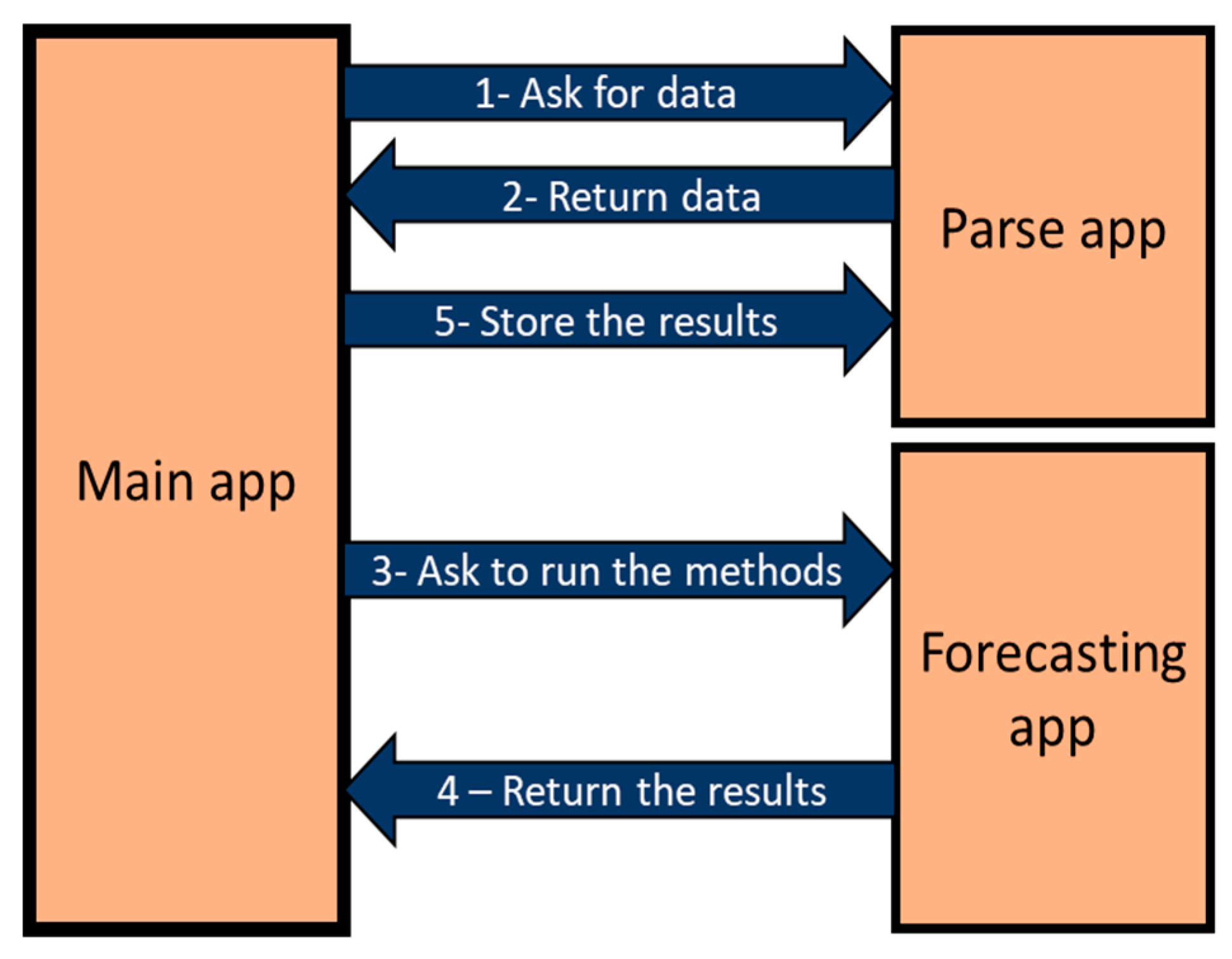
The main app is the central component of the application which connects the other two components. All the communications between the user and the application are a part of the responsibilities of the main app. Once the user chooses a date to start a forecasting process, the main app makes a connection to the parse app and asks for the needed data from the chosen date to run the forecasting algorithms. After receiving the data, the main app sends this data to the forecasting app. The forecasting app runs the forecasting methods by the received data from the main app and returns the results of the forecasting. The main app shows the results to the user and sends them to the parse app to be stored. Figure 4 presents the connections between the components of the application.

The forecasting app is based on the java and R programming languages and is responsible to receive the data from the main app and run the forecasting methods. This component of the application includes the implementation of the forecasting methods. Every algorithm has its own class which creates a connection to the R programing language to run the methods in this language. There are two available ways to run the methods. The first is run the algorithms by an excel file that the user should insert; and the second way is an automatic forecasting, in which the user chooses a date and hour and the application does the forecast automatically, the second way is where the application asks for data from parse app. For every forecasting method, there are two R scripts one for automatic forecasting and one for forecasting by an excel file. 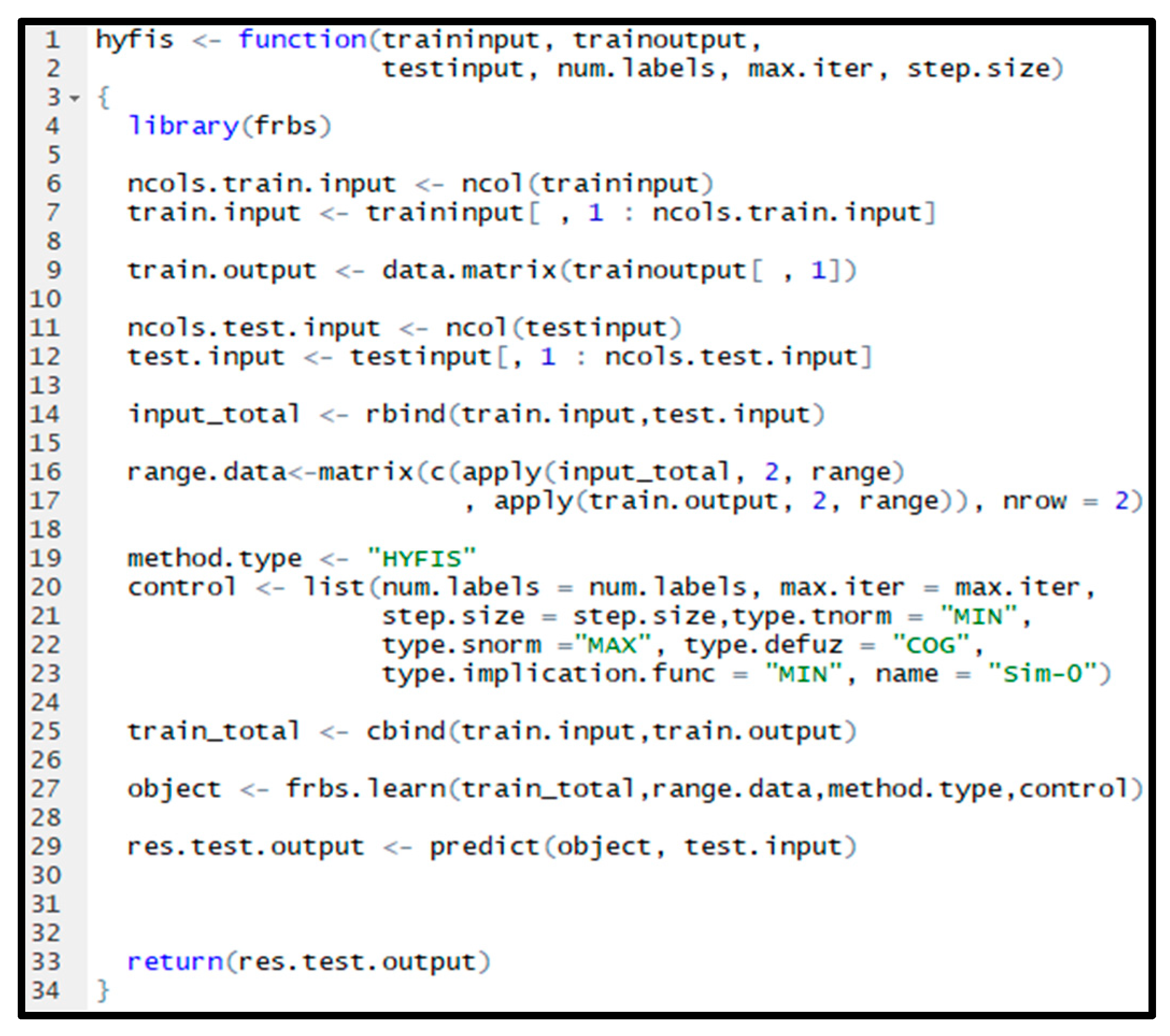Figure 5 presents the R script of HyFIS method in case of automatic forecasting, where the FRBS library [29] is used to implement this method.

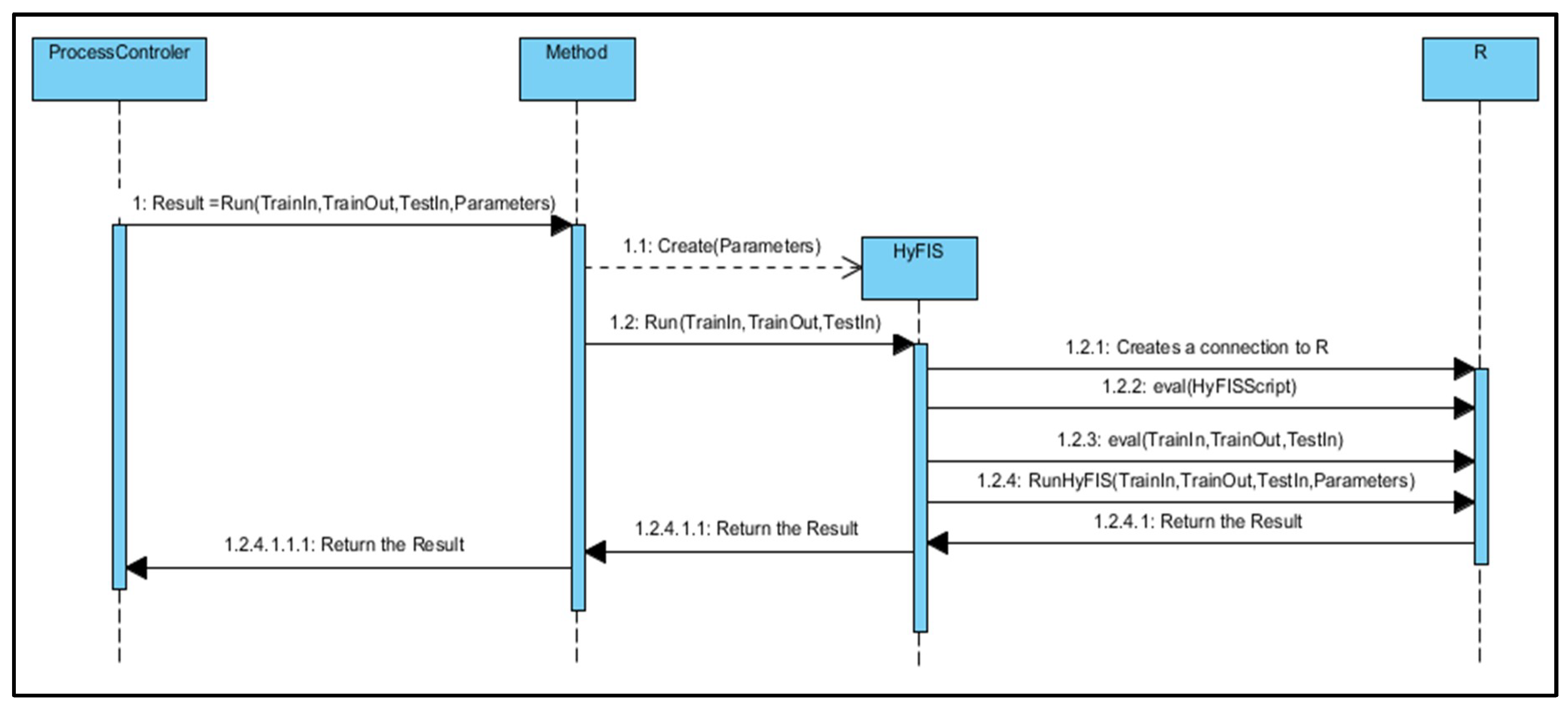
As it is visible in Figure 5, the hyfiz function in R receives three data sets as well as the needed variables to configure the method that the user can insert during the process of the forecasting. The traininput and trainoutput are used as the training data, and the testinput is meant to be used as the test data. Figure 6 presents the sequence of running the HyFIS method in R language.

Parse app includes the implementation of the forecasting strategies, all the connections to the databases and the data storage processes. Every proposed forecasting strategy has its own class which is connected to the databases connection classes. Every time the user chooses a date and a strategy to run the forecasting process, this date will be sent to the class of the deliberate strategy. This class asks for the required data from the database connection classes and creates the needed data sets to forecast the energy consumption of the inserted hour by the chosen strategy. Once the application creates these data sets, it stores these data so the next time the application does not need to ask from the database for the data. This data storage process helps the application to reduce the duration of the expectation.

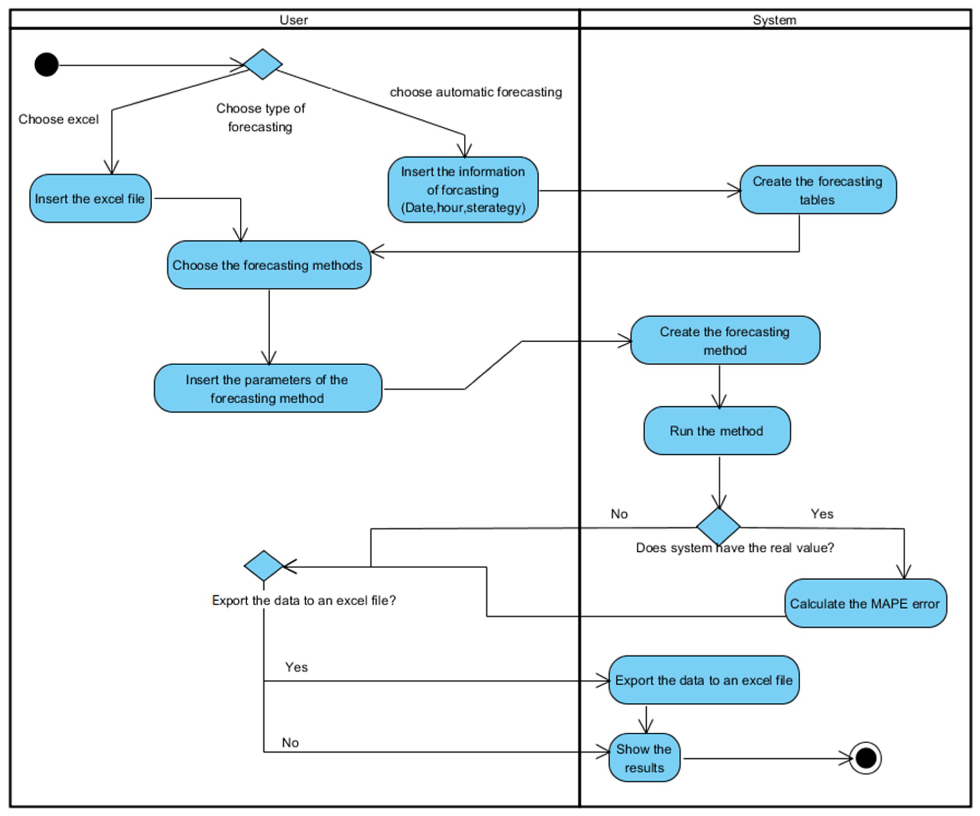
The main app is the central component of the application. The communications between the user and the application are included in this part as well as the communications between two other components of the application and the controller classes. Figure 7 presents the activity diagram of the application where the sequence of the forecasting process is presented.

As it is visible in Figure 7 when the forecasting methods return the predicted results in the case that the real value of the forecasting target is available the application also calculates the Mean Absolute Percentage Error (MAPE) of the predicted value and present it to the user. Also, at the end of the process in case of the automatic forecasting, the user can ask to export the forecasting data sets and the result to an excel file.

3.3. Graphical User Interface

The graphical user interface of this application is implemented based on JavaFX, which is a set of graphics and media APIs that can be used to create and deploy rich client applications. It allows developers to build rich cross-platform applications rapidly and supports modern GPUs through hardware-accelerated graphics [39]. This section includes a sequence of figures which present the different pages of the application.

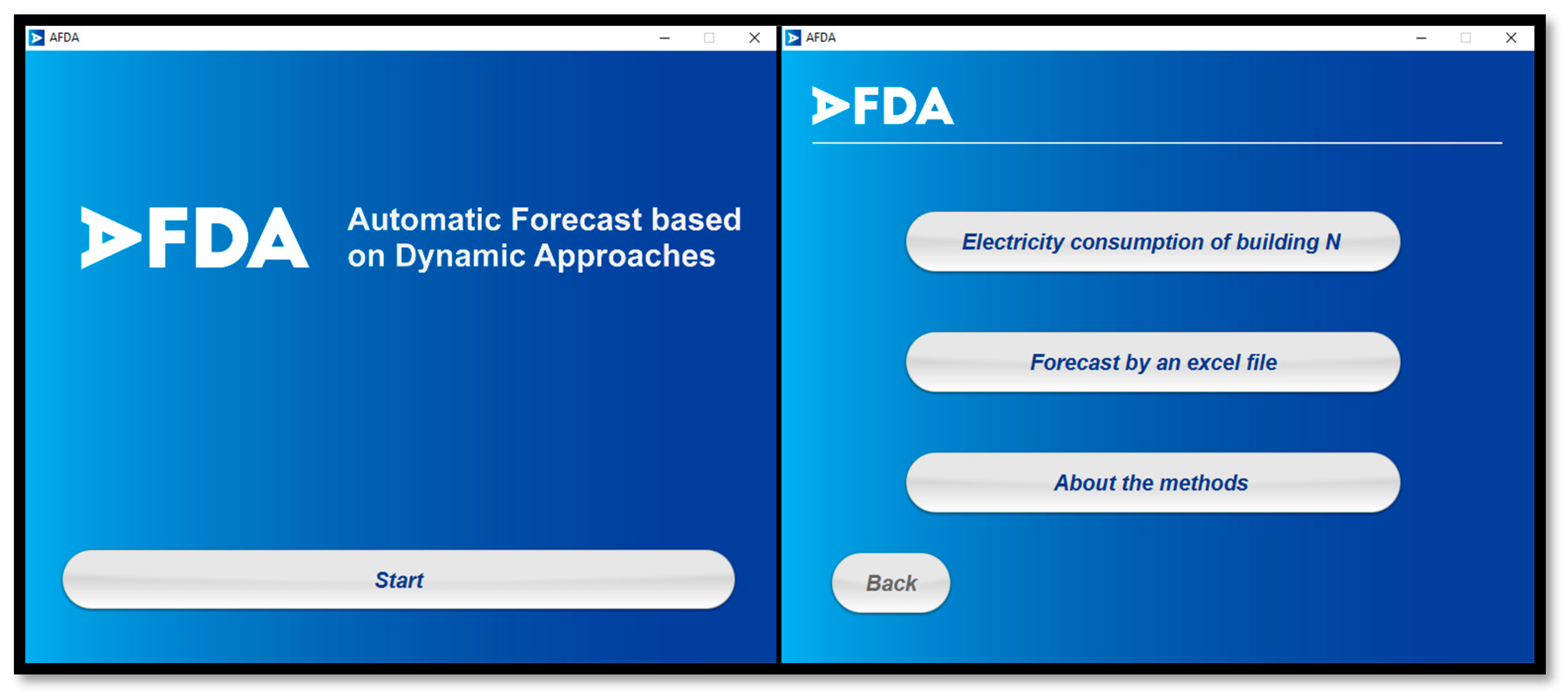
The application has a main page that opens when the user runs the application. This page includes the name of the application and the information about it as well as a start bottom. When the user starts the application the main menu of the application will open. Figure 8 presents the main page and the main menu of the application.

The first bottom of the menu opens the menu of the building N, the second one starts the process of forecasting by an excel file, and the third bottom opens a menu where the user has a brief explanation about the forecasting methods.

As you can see in Figure 9, the menu of the building N, includes all the use cases that are related to the building N, including, forecasting the electricity consumption, get the real data and list all the forecasted values.

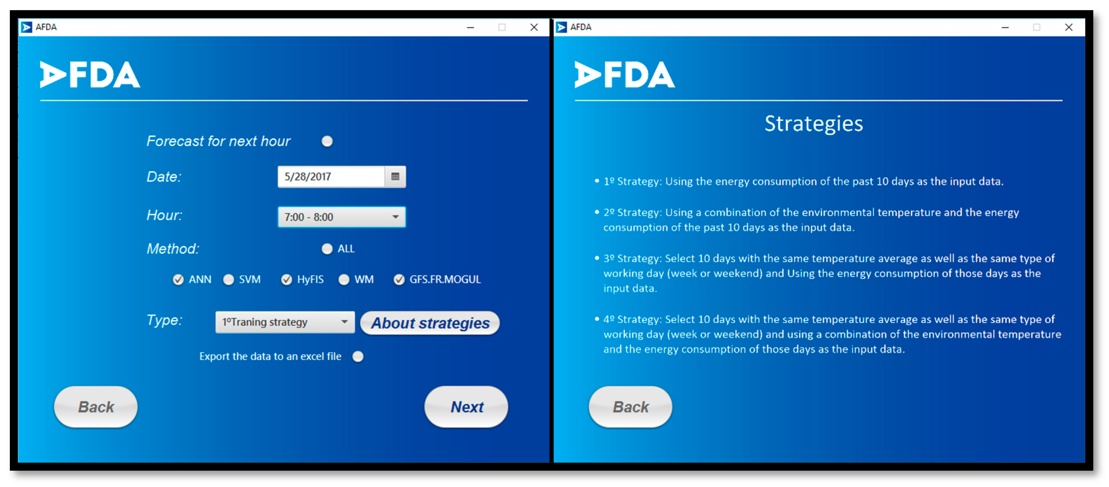
In case the user selects the first bottom, the process of the forecasting the electricity consumption of the building N will start. It opens a page where the user should choose a date, an hour, the training strategy, and at least one forecasting method. This page includes a bottom that opens an explanation of the strategies. Figure 10 presents these two pages.

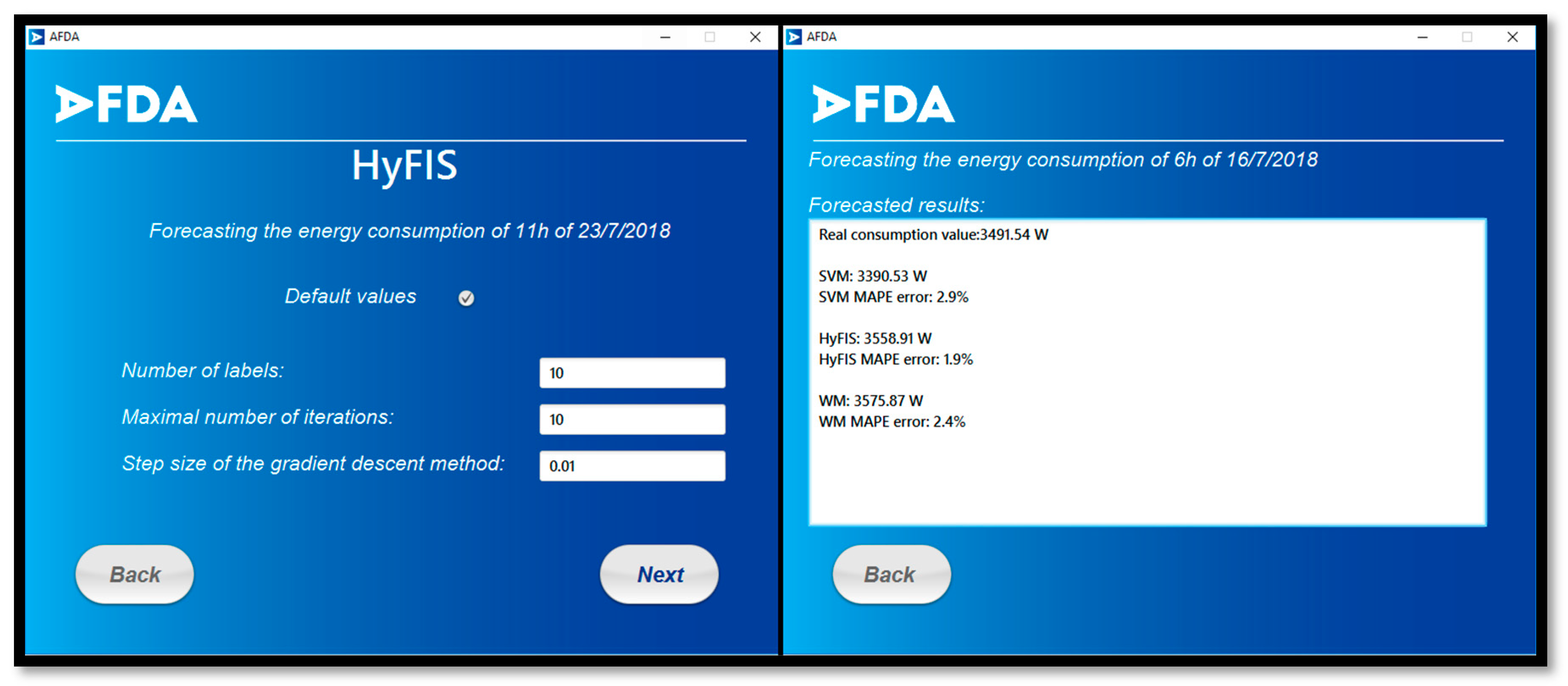
In the next step, the user must insert the required variables to configure the forecasting model. For each selected method, a page will appear where the user can introduce these values or select an option to use the default values of the application. At the end of this process the application presents the predicted result. In a case that the application has access to the real value of the target value, the MAPE error of the results will be presented as well. Figure 11 presents these two phases.

4. Case Study

This section presents a case study in order to evaluate the performance of the proposed application, by assessing the accuracy of the proposed forecasting methods namely ANN [16], SVM [40], HyFIS [31], WM [33], GFS.FR.MOGUL [36] and verify the influence of using different training strategies on the performance of the forecasting process. This case study includes the hour-ahead prediction of the energy consumption of GECAD’s building N during 24 h of a business day. The electricity consumption is forecasted based on 4 forecasting strategies using 5 forecasting algorithms from the proposed application.

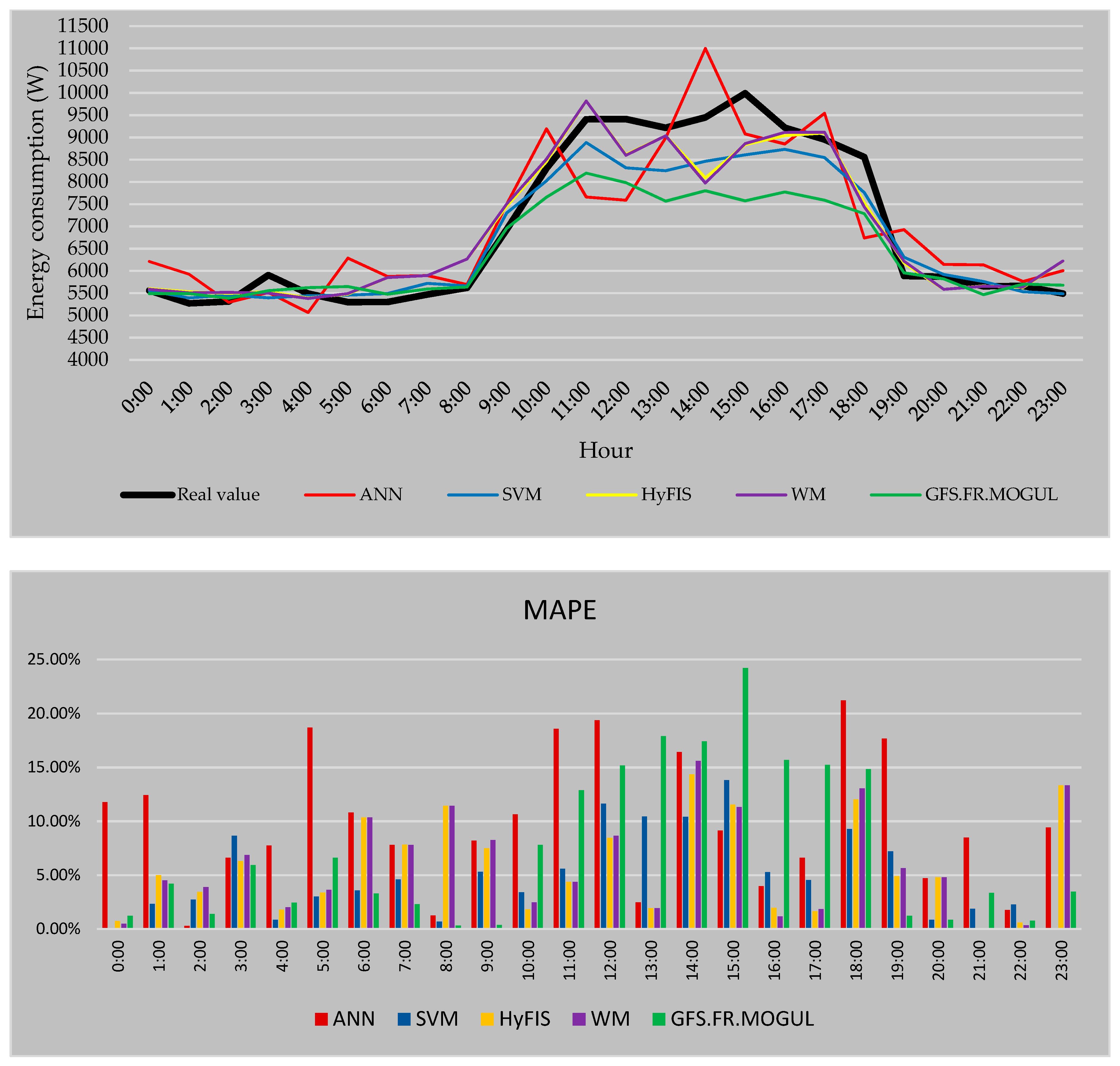
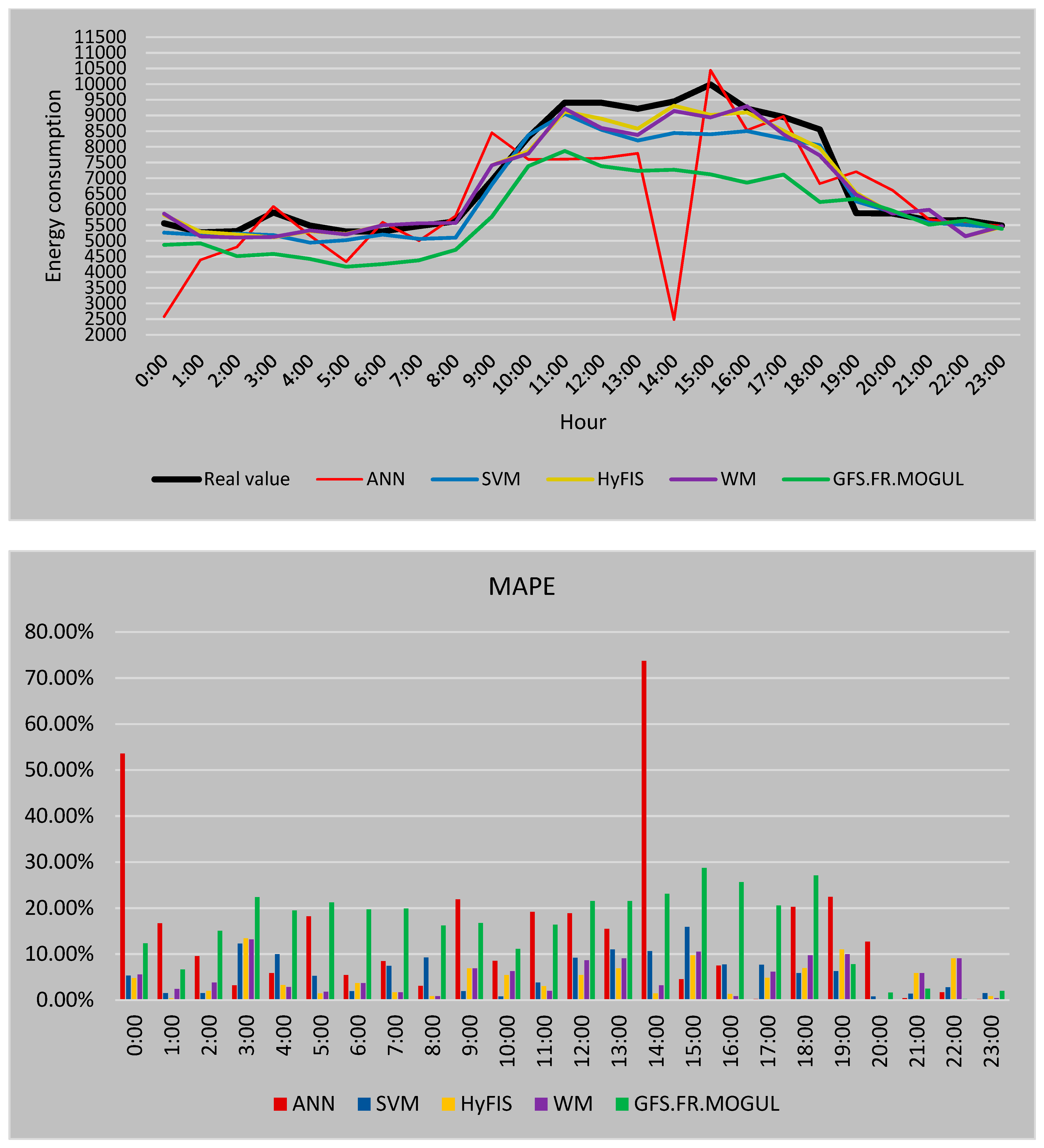
Figure 12 represents a comparison between the forecasted electricity consumption for 24 h of 2018/4/6 using 5 forecasting methods based on the first training strategy as well as the real consumption values. In this strategy, the methods are trained by the electricity consumption of the 10 past days before the target day.

In Figure 12 the real consumption value of every hour is presented by the black line. As it is visible, during the peak hours of the consumption the predicted values are mostly lower than the real value. The MAPE is used to measure the accuracy of the forecasted values. For this strategy, the most reliable values by the average error of 4.93% are calculated by SVM followed by HyFIS with 5.81% and WM with 5.99%. Also, the GFS.FR.MOGUL by 7.45% error and ANN by 9.83% are the methods by the highest error in the case of the first forecasting strategy.

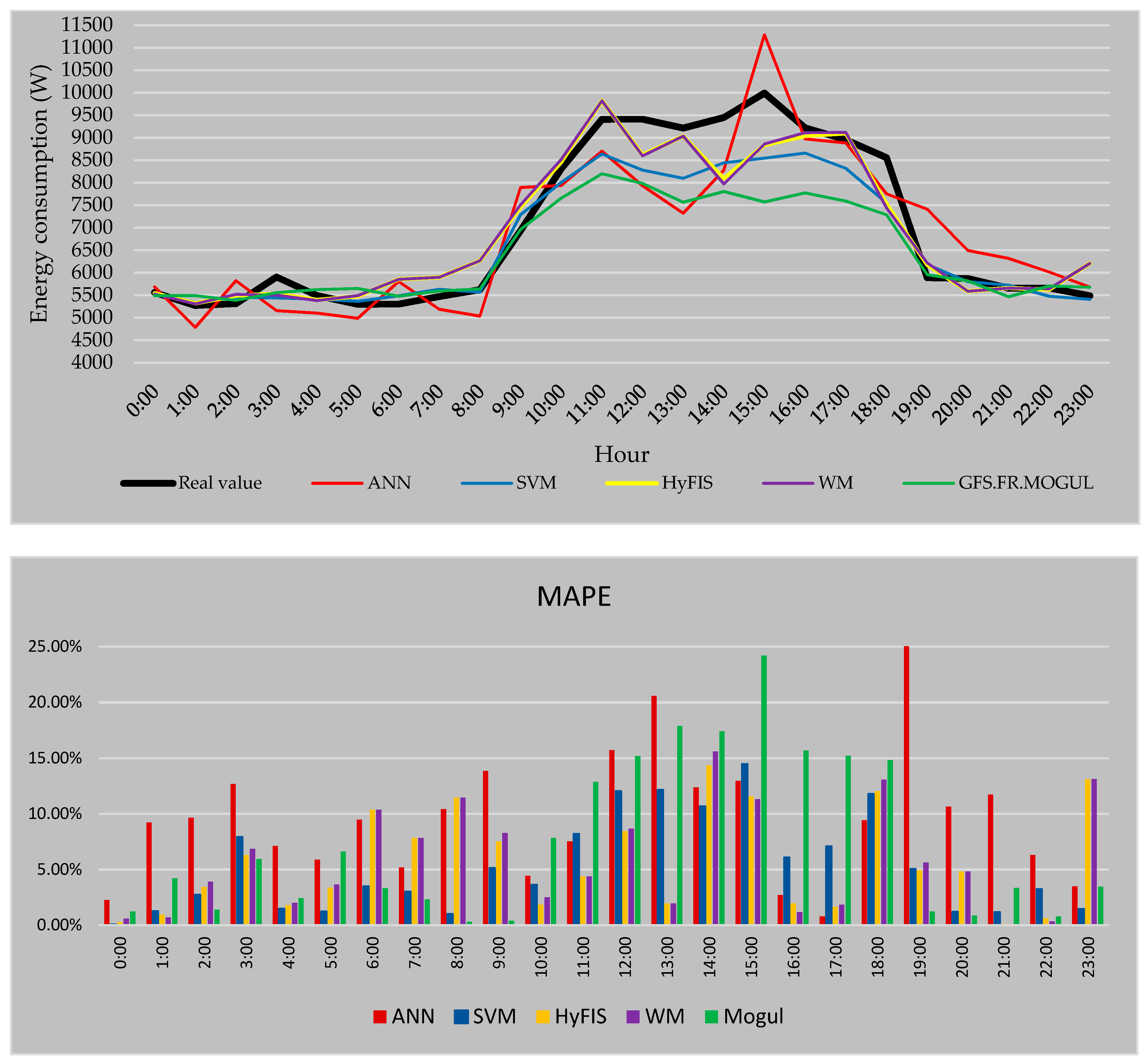
Figure 13 presents the forecasted results by the methods while using the second forecasting strategy to train the methods. The comparison between these results and the forecasted values by the first strategy shows that in the case of GFS.FR.MOGUL the results are the same and using the environmental template has no influence on the performance of this method and the error is still 7.45%. ANN by 9.58%, HyFIS by 5.61% and WM by 5.82% of MAPE error while using the second strategy, have a more reliable result than when the first strategy is used. The only method that has a higher error when the environmental temperature is used in the training data is SVM by the error of 5.21%; however, SVM still has the best result in the case of this strategy.

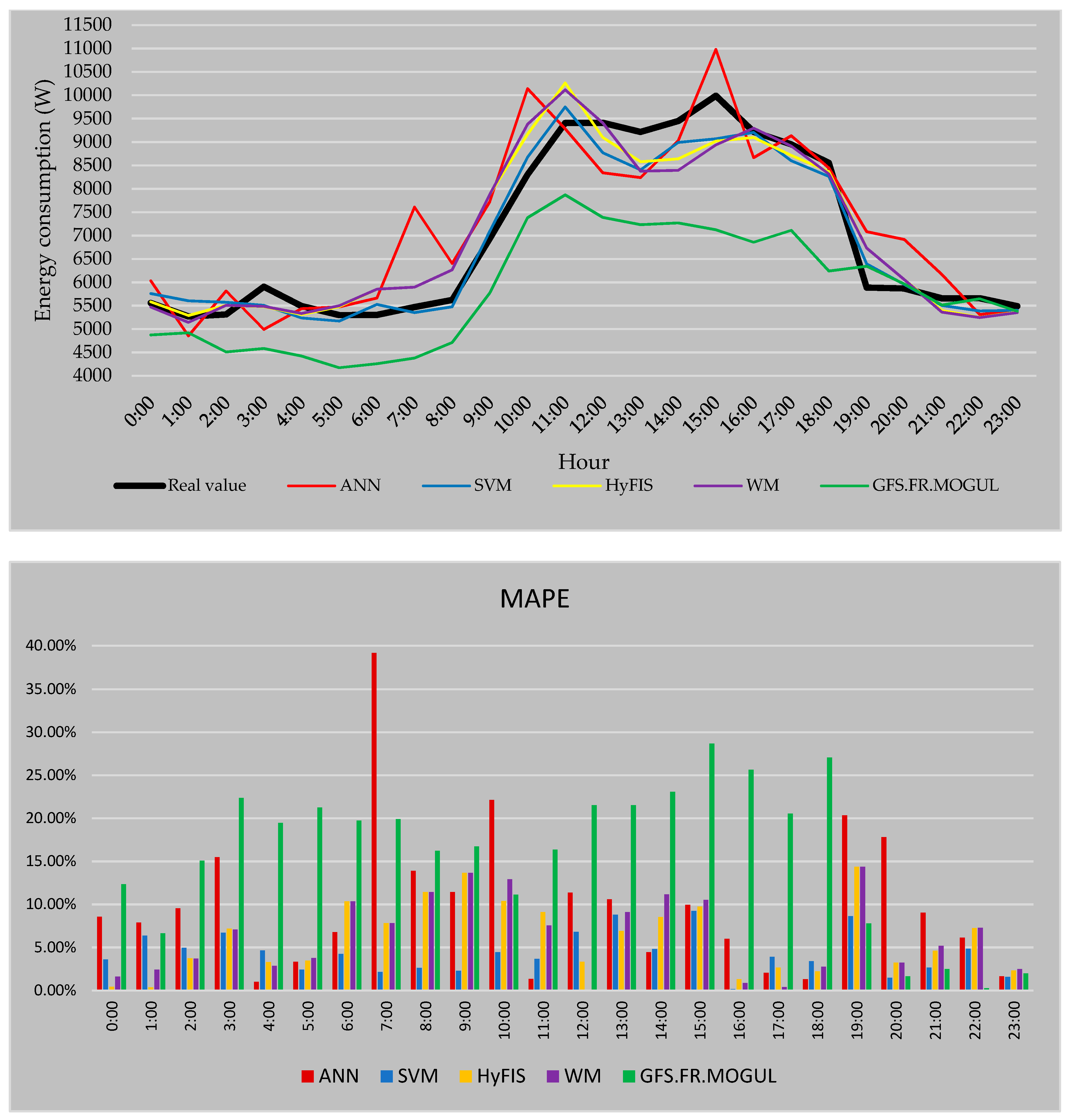
Figure 14 includes the forecasting result of the third strategy.

As can be seen in the results of Figure 14, the GFS.FR.MOGUL in the most hours, predicts a much lower value than the real value which eventuates an error of 15.8% for this method when the third strategy is used. HyFIS and WM by an average error of 6.15% and 6.35% also have a higher error for this strategy compared to the errors of the first and second ones. For ANN, the calculated error is 10% which is a better error than the error of this method when the second strategy is used but the performance of this method when the first strategy has been used, stills the best performed results by this method. In contrast, the SVM by the error of 4.34% while the third strategy is used has the best results between the forecasting methods and has the best predicted results by SVM between these forecasting strategies.

As one can see in Figure 15, the predicted results by ANN when the fourth strategy is used have a high variation and, in some cases, the method predicts a much lower value than the real value. The average MAPE error for the ANN using the fourth strategy is 14.64%, which is the worst performed value by this method. As it has been proved, using the environmental temperature in the training data has no effect on the results of GFS.FR.MOGUL, and this method has the same error as the third strategy which is 15.8%. When the fourth strategy is used, the HyFIS has the best error by an average error of 4.58% followed by WM with 5.19% and SVM by 5.9%.

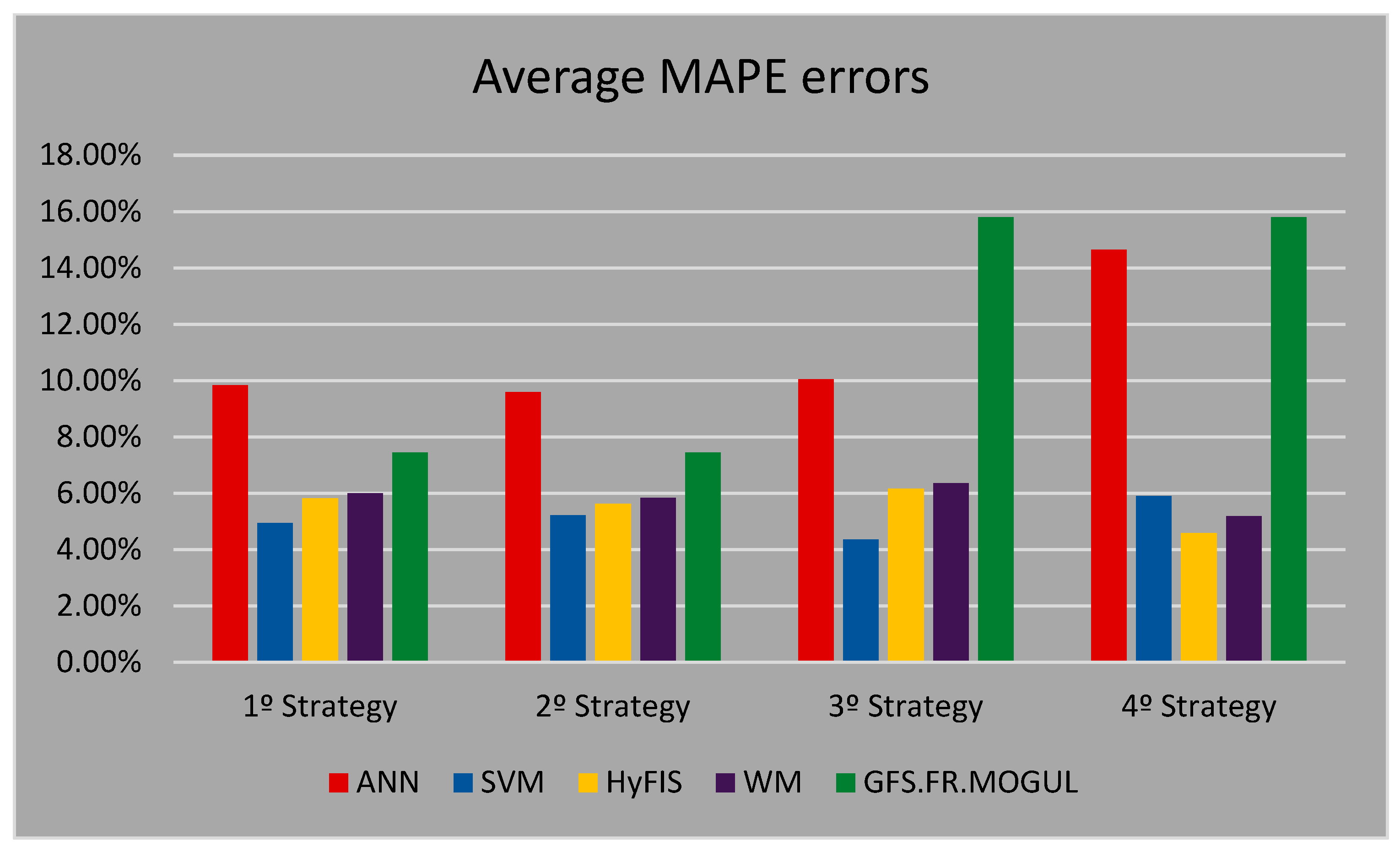
Figure 16 presents a comparison between the average MAPE error of the forecasting methods based on the four proposed forecasting strategies in this work.

It is not possible to conclude that there is an absolute forecasting strategy that has the best result for all the forecasting methods. For ANN, the best strategy is the first one, which has the simplest data set. About GFS.FR.MOGUL it is possible to say that using the environmental temperature has no influence on the results of this method. On the other hand, the process of selecting the particular date to collect the train data has a negative effect on the performance of this method. This way the best forecasting strategy for the GFS.FR.MOGUL is also the first one. The HyFIS and WM have similar efficiency. These two methods can predict a more reliable value when the environmental temperature is used in the train data. This conclusion is valid in both cases of the second and fourth strategy. The best calculated results from these two methods are when the fourth strategy is used. The HyFIS by using the fourth strategy has the second-best calculated error in this work. The SVM has the most stable and trustable results while different forecasting strategies are used. This method has the most accurate result in the case of three of four proposed forecasting strategies in this work. SVM by an error of 4.35% when the third strategy is used has the best calculated error in this case study.

5. Conclusions

This paper presents an automatic forecasting application based on Java and R programming languages. By using this application, the user can create different forecasting models using five forecasting methods and four data preparation strategies to predict the hour-ahead energy consumption of an office building. ANN, SVM, HyFIS, WM, and GFS.FR.MOGUL are the considered forecasting algorithms in this work as well as four data preparation strategies which are explained in Section 2. The most important advantage that this application offers is that the user does not need to have knowledge about the programming languages, forecasting technics, and data storage systems and all the process is done by the application. Additionally, by making different algorithms and data treatment strategies available, the proposed work also enables the user to find the best method to be used in distinct prediction conditions. This is especially relevant considering that by being domain-agnostic, the proposed application can be applied to multiple application domains, such as manufacturing systems, health related management systems, internet-of-things problems, or many other problems that require forecasting solutions based on historical data regression.

The presented case studies using this application show that the proposed approaches in this work can forecast the hour-ahead energy consumption with acceptable performance. The SVM with the third proposed data preparation strategy presents an error of 4.35% which is a trustable performance compared to the other methods and previous work. Moreover, when using additional information for training, in this case, the temperature, as input for consumption forecasting, it is visible that both the HyFIS and WM can improve their results and reach better results than the SVM (in specific, using the 4th data strategy). Hence, the application can support users’ decisions on the best method, parameterization, and data treatment that should be used depending on the available data.

As future work, further forecasting methods will be included, to broaden the available learning capabilities from various methods. Probabilistic forecasting will also be included, as well as the possibility of working with other types of data and databases, not necessarily related to energy consumption.

References

1. Peng, T.M.; Hubele, N.F.; Karady, G.G. Advancement in the application of neural networks for short-term load forecasting. Power Syst. IEEE Trans. 1992, 7, 250–257. [Google Scholar] [CrossRef]
2. Pang, C.K.; Sheble, G.B.; Albuyeh, F. Evaluation of Dynamic Programming Based Methods and Multiple Area Representation for Thermal Unit Commitments. IEEE Trans. Power Appar. Syst. 1981, PAS-100, 1–100. [Google Scholar] [CrossRef]
3. Hara, K.; Kimura, M.; Honda, N. A Method for Planning Economic Unit Commitment and Maintenance of Thermal Power Systems. IEEE Trans. Power Appar. Syst. 1966, PAS-85, 427–436. [Google Scholar] [CrossRef]
4. Khosravani, H.; Castilla, M.; Berenguel, M.; Ruano, A.; Ferreira, P. A Comparison of Energy Consumption Prediction Models Based on Neural Networks of a Bioclimatic Building. Energies 2016, 9, 57. [Google Scholar] [CrossRef]
5. Directive 2010/31/EU the Directive 2010/31/EU of the European Parliament and of the Council of 19 May 2010 on the energy performance of buildings. Off. J. Eur. Union L153 2010, 18, 2010.
6. Liang, J.; Du, R. Model-based Fault Detection and Diagnosis of HVAC systems using Support Vector Machine method. Int. J. Refrig. 2007, 30, 1104–1114. [Google Scholar] [CrossRef]
7. Zhao, H.X.; Magoulès, F. A review on the prediction of building energy consumption. Renew. Sustain. Energy Rev. 2012, 16, 3586–3592. [Google Scholar] [CrossRef]
8. Mena, R.; Rodríguez, F.; Castilla, M.; Arahal, M.R. A prediction model based on neural networks for the energy consumption of a bioclimatic building. Energy Build. 2014, 82, 142–155. [Google Scholar] [CrossRef]
9. Buhan, S.; Cadirci, I. Multistage Wind-Electric Power Forecast by Using a Combination of Advanced Statistical Methods. IEEE Trans. Ind. Inform. 2015, 11, 1231–1242. [Google Scholar] [CrossRef]
10. Liu, H.; Erdem, E.; Shi, J. Comprehensive evaluation of ARMA--GARCH (-M) approaches for modeling the mean and volatility of wind speed. Appl. Energy 2011, 88, 724–732. [Google Scholar] [CrossRef]
11. Kavasseri, R.G.; Seetharaman, K. Day-ahead wind speed forecasting using f-ARIMA models. Renew. Energy 2009, 34, 1388–1393. [Google Scholar] [CrossRef]
12. Louka, P.; Galanis, G.; Siebert, N.; Kariniotakis, G.; Katsafados, P.; Pytharoulis, I.; Kallos, G. Improvements in wind speed forecasts for wind power prediction purposes using Kalman filtering. J. Wind Eng. Ind. Aerodyn. 2008, 96, 2348–2362. [Google Scholar] [CrossRef] [Green Version]
13. Wilamowski, B.M.; Yu, H. Neural network learning without backpropagation. IEEE Trans. Neural Netw. 2010, 21, 1793–1803. [Google Scholar] [CrossRef]
14. Boser, B.E.; Guyon, I.M.; Vapnik, V.N. A training algorithm for optimal margin classifiers. In Proceedings of the Fifth Annual Workshop on Computational Learning Theory, Pittsburgh, PA, USA, 27–29 July 1992; pp. 144–152. [Google Scholar]
15. Zadeh, L.A. Fuzzy sets. Inf. Control 1965, 8, 338–353. [Google Scholar] [CrossRef] [Green Version]
16. Vinagre, E.; Gomes, L.; Vale, Z. Electrical Energy Consumption Forecast Using External Facility Data. In Proceedings of the 2015 IEEE Symposium Series on Computational Intelligence, Cape Town, South Africa, 7–10 December 2015; pp. 659–664. [Google Scholar]
17. Jozi, A.; Pinto, T.; Praça, I.; Ramos, S.; Vale, Z.; Goujon, B.; Petrisor, T. Energy Consumption Forecasting using Neuro-Fuzzy Inference Systems: Thales TRT building case study. In Proceedings of the 2017 IEEE Symposium Series on Computational Intelligence (SSCI), Honolulu, HI, USA, 27 November–1 December 2017. [Google Scholar]
18. Torbat, S.; Khashei, M.; Bijari, M. A hybrid probabilistic fuzzy ARIMA model for consumption forecasting in commodity markets. Econ. Anal. Policy 2018, 58, 22–31. [Google Scholar] [CrossRef]
19. Ruiz, L.G.B.; Rueda, R.; Cuéllar, M.P.; Pegalajar, M.C. Energy consumption forecasting based on Elman neural networks with evolutive optimization. Expert Syst. Appl. 2018, 92, 380–389. [Google Scholar] [CrossRef]
20. Pinto, T.; Ramos, S.; Sousa, T.M.; Vale, Z. Short-term wind speed forecasting using Support Vector Machines. In Proceedings of the IEEE Symposium on Computational Intelligence in Dynamic and Uncertain Environments (CIDUE), Orlando, FL, USA, 9–12 December 2014; pp. 40–46. [Google Scholar]
21. Lago, J.; De Ridder, F.; Vrancx, P.; De Schutter, B. Forecasting day-ahead electricity prices in Europe: The importance of considering market integration. Appl. Energy 2018, 211, 890–903. [Google Scholar] [CrossRef] [Green Version]
22. Cerne, G.; Dovzan, D.; Skrjanc, I. Short-term load forecasting by separating daily profile and using a single fuzzy model across the entire domain. IEEE Trans. Ind. Electron. 2018, 65, 7406–7415. [Google Scholar] [CrossRef]
23. Osorio, G.J.; Matias, J.C.O.; Cataläo, J.P.S. Short-term wind power forecasting using adaptive neuro-fuzzy inference system combined with evolutionary particle swarm optimization, wavelet transform and mutual information. Renew. Energy 2014, 75, 311. [Google Scholar] [CrossRef]
24. Renna, P. Energy saving by switch-off policy in a pull-controlled production line. Sustain. Prod. Consum. 2018, 16, 25–32. [Google Scholar] [CrossRef]
25. Lechler, A.; Verl, A. Control-integrated consumption graph-based optimisation method for energy reduction of machine tools with automated parameter optimisation AU—Eberspächer, Philipp. Int. J. Comput. Integr. Manuf. 2016, 29, 1307–1316. [Google Scholar]
26. Mandal, P.; Senjyu, T.; Urasaki, N.; Funabashi, T.; Srivastava, A.K. A novel approach to forecast electricity price for PJM using neural network and similar days method. IEEE Trans. Power Syst. 2007, 22, 2058–2065. [Google Scholar] [CrossRef]
27. Schaefer, A.M.; Udluft, S.; Zimmermann, H.-G. A Recurrent Control Neural Network for Data Efficient Reinforcement Learning. In Proceedings of the 2007 IEEE International Symposium on Approximate Dynamic Programming and Reinforcement Learning, Honolulu, HI, USA, 1–5 April 2007; pp. 151–157. [Google Scholar]
28. Vapnik, V. Pattern recognition using generalized portrait method. Autom. Remote Control 1963, 24, 774–780. [Google Scholar]
29. Pinto, T.; Sousa, T.M.; Praça, I.; Vale, Z.; Morais, H. Support Vector Machines for decision support in electricity markets’ strategic bidding. Neurocomputing 2016, 172, 438–445. [Google Scholar] [CrossRef]
30. Riza, L.S.; Bergmeir, C.; Herrera, F.; Benítez, J.M. FRBS: Fuzzy Rule-Based Systems for Classification and Regression in R. J. Stat. Softw. 2015, 65. [Google Scholar] [CrossRef]
31. Kim, J.; Kasabov, N. HyFIS: Adaptive neuro-fuzzy inference systems and their application to nonlinear dynamical systems. Neural Netw. 1999, 12, 1301–1319. [Google Scholar] [CrossRef]
32. Jozi, A.; Pinto, T.; Praca, I.; Silva, F.; Teixeira, B.; Vale, Z. Energy consumption forecasting based on Hybrid Neural Fuzzy Inference System. In Proceedings of the 2016 IEEE Symposium Series on Computational Intelligence (SSCI), Athens, Greece, 6–9 December 2016; pp. 1–5. [Google Scholar]
33. Kato, E.R.R.; Morandin, O.; Sgavioli, M.; Muniz, B.D. Genetic tuning for improving Wang and Mendel’s fuzzy database. In Proceedings of the IEEE International Conference on Systems, Man and Cybernetics, San Antonio, TX, USA, 11–14 October 2009; pp. 1015–1020. [Google Scholar]
34. Jozi, A.; Pinto, T.; Praça, I.; Silva, F.; Teixeira, B.; Vale, Z. Wang and Mendel’s Fuzzy Rule Learning Method for Energy Consumption Forecasting considering the Influence of Environmental Temperature. In Proceedings of the lobal Information Infrastructure and Networking Symposium (GIIS), Porto, Portugal, 19–21 October 2016. [Google Scholar]
35. Herrera, F.; Lozano, M.; Verdegay, J.L. A Learning Process for Fuzzy Control Rules using Genetic Algorithms. Fuzzy Sets Syst. 1995, 100, 143–158. [Google Scholar] [CrossRef]
36. FJozi, A.; Pinto, T.; Praça, I.; Silva, F.; Teixeira, B.; Vale, Z. Energy Consumption Forecasting using Genetic fuzzy rule-based systems based on MOGUL Learning Methodology. In Proceedings of the IEEE Manchester PowerTech, Manchester, UK, 18–22 June 2017. [Google Scholar]
37. Weather Underground. Available online: https://www.wunderground.com/ (accessed on 1 January 2019).
38. Meteo ISEP. Available online: https://meteo.isep.ipp.pt/gauges (accessed on 1 January 2019).
39. ORACLE JavaFX. Available online: https://www.oracle.com/technetwork/java/javafx/overview/index.html (accessed on 1 January 2019).
40. Vinagre, E.; Pinto, T.; Ramos, S.; Vale, Z.; Corchado, J.M. Electrical Energy Consumption Forecast Using Support Vector Machines. In Proceedings of the 2016 27th International Workshop on Database and Expert Systems Applications (DEXA), Porto, Portugal, 5–8 September 2016; pp. 171–175. [Google Scholar]
Figure 1. A general schematic diagram of the HyFIS.
Applsci 09 00699 g001
Figure 2. The structure of the Neuro-Fuzzy model from the HyFIS architecture.
Applsci 09 00699 g002
Figure 3. The sequence of fuzzy rules creation in WM method.
Applsci 09 00699 g003
Figure 4. A generic model of the implementation.
Applsci 09 00699 g004
Figure 5. R script of HyFIS forecasting method.
Applsci 09 00699 g005
Figure 6. The sequence diagram in the case of using the HyFIS method.
Applsci 09 00699 g006
Figure 7. Activity diagram of the application.
Applsci 09 00699 g007
Figure 8. The principal page and menu of the application.
Applsci 09 00699 g008
Figure 9. The menu of the Building N.
Applsci 09 00699 g009
Figure 10. The Information picker and strategies explanation pages.
Applsci 09 00699 g010
Figure 11. The method creation and results presentation pages.
Applsci 09 00699 g011
Figure 12. Forecasted values and error of the methods using the 1st data preparation strategy.
Applsci 09 00699 g012
Figure 13. Forecasted values and error of the methods using the 2st data preparation strategy.
Applsci 09 00699 g013
Figure 14. Forecasted values and errors for building N using the 3rd data preparation strategy.
Applsci 09 00699 g014
Figure 15. Forecasted values and error of the methods using the 4th data preparation strategy.
Applsci 09 00699 g015
Figure 16. Average MAPE errors of the forecasting methods.
Applsci 09 00699 g016