Article

Simultaneous OTDR Dynamic Range and Spatial Resolution Enhancement by Digital LFM Pulse and Short-Time FrFT

Wuhan National Laboratory for Optoelectronics, Huazhong University of Science and Technology, Wuhan 430074, China
*
Author to whom correspondence should be addressed.
Appl. Sci. 2019, 9(4), 668; https://doi.org/10.3390/app9040668
Submission received: 21 December 2018 / Revised: 1 February 2019 / Accepted: 12 February 2019 / Published: 15 February 2019
(This article belongs to the Special Issue Optical Correlation-domain Distributed Fiber Sensors)

Abstract

:
This paper proposes a novel optical time domain reflectometry (OTDR) method based on the digital linear frequency modulation (LFM) pulse, which can achieve a tradeoff between maximum measurable distance and spatial resolution. Direct modulation and detection are adopted at the transmitting and receiving ends, respectively, which is simple in construction and does not require additional optics. The short-time fractional Fourier transform (STFrFT) is introduced for the signal processing and noise filtering. The theoretical analysis of the working principle confirmed that the spatial resolution is determined by the sweep frequency range of the digital LFM signal rather than the pulse width. The influence of the STFrFT window on the peak sidelobe ratio of the reflection peak is also studied. By combining STFrFT and sidelobe suppression, the dynamic range and spatial resolution can be appreciably enhanced simultaneously. In the demo experiments testing the proposed method on a conventional OTDR development board for comparison, a 7-dB improvement in the dynamic range and an approximately 10-times improvement in the spatial resolution are simultaneously achieved.

1. Introduction

Optical time domain reflectometry (OTDR) is a common technique for measuring the optical fiber length, attenuation and insertion loss of connectors, splices and breakpoints. It operates by injecting probe optical pulses into the fiber under test (FUT) and successively detecting the backscattered optical power with the round-trip time [1,2]. OTDR is widely used in passive optical networks (PONs) for fault detection, localization and identification [3,4].
With the rapid development of PONs, OTDR methods with high dynamic range and spatial resolution are crucial for their monitoring. There are three main ways of improving the OTDR dynamic range: (1) increasing the energy of the probe optical pulse, (2) improving the receiver sensitivity [5,6,7,8], and (3) adopting pulse coding techniques [9,10,11]. The first one can be actuated in two manners. One involves using a high-power laser but incurs high costs, and the increased optical power injected into the FUT would cause nonlinear effects, such as stimulated Brillouin scattering [12] and modulation nonlinearities [13], affecting the detection of backscattered light. The other involves increasing the duration of the forward probe pulse, but this would deteriorate the spatial resolution, affecting the OTDR performance and fault localization accuracy. The second approach is mainly realized using cryogenic detectors, photon counters and coherent detection. Cryogenic detectors and photon counters are not suitable for practical applications due to their costs and cooling requirements [14]. Therefore, coherent detection seems the most practical method to achieve high receiver sensitivity. Unfortunately, its detection distance is limited by factors such as the coherence length of the light source, phase noise and polarization state of the backscattered light [15]. In the third approach, the optical pulse is encoded and successively injected into FUT as a probe signal. The backscattering curve is derived from the received backscattered signal via the correlation operation, which is equivalent to injecting a narrower probe pulse with the same energy. However, given the logarithmic relation between the encoding gain and length of the encoding OTDR, it is useless to keep increasing the encoding length above 256 bits to improve the encoding gain [16].
In the conventional OTDR, the spatial resolution is determined by the pulse width. The optical frequency domain reflectometry (OFDR) based on the Fourier transform has been proposed to solve this problem [17,18]; a tunable light source is employed to generate a probe signal with a periodic optical linear frequency modulation (LFM), and the information on FUT can be obtained by analyzing the backscattered light in the frequency domain. The OFDR spatial resolution is determined by the sweep frequency range of the LFM signal rather than the pulse width. Therefore, OFDR can overcome the conflict between spatial resolution and pulse width of the conventional OTDR. However, there are also some problems with OFDR using coherent detection. Firstly, the OFDR detection distance is usually limited to only a few hundred meters because of the coherence length and phase noise of the laser source and the randomly changing polarization state of the backscattered light [19,20]. Secondly, improving the OFDR performance usually requires the use of a laser with small phase noise and narrow linewidth, but such lasers are generally characterized by large volumes, low output optical powers and high costs. Recently, based on the concept of LFM pulse compression radar, an optical pulse compression reflectometry (OPCR) has been proposed [21]. The OPCR uses optical probe pulses with LFM and then uses a matched filter to realize pulse compression on the received backscatter trace. As with the OFDR, the spatial resolution of the OPCR is also only determined by the sweep frequency range of the LFM signal. Unfortunately, due to the influence of the laser phase noise and the random variation of the polarization state, the OPCR measuring distance was only 5.4 km [21,22]. In summary, OFDR and OPCR are not suitable for applications in optical fiber communication systems, especially for cost-sensitive PONs.
This paper proposes a novel OTDR method, called digital LFM OTDR (DLFM–OTDR), which can be considered a new pulse coding technique, but it has different performance than the previous pulse coding technique. It combines the advantages of the conventional OTDR and OFDR. Based on the pulse coding technique with the modulated signal as a digital LFM signal, the probe signal is directly modulated at the transmitting end. There is no need for additional optical equipment, which is bulky and unsuitable for portable OTDRs, to modulate the frequency of the signal light as with OPCR. Additionally, direct detection at the receiving end is adopted. Thus, the DLFM–OTDR can overcome the shortcomings of OFDR and OPCR. The measurement curve is affected neither by the phase noise and coherence length of the laser nor by the changes in the polarization state of the backscattered light. Moreover, DLFM–OTDR can simultaneously overcome the contradiction between the spatial resolution and measurement distance of the conventional OTDR by using the digital LFM probe signal and the short-time fractional Fourier transform (STFrFT) [23,24]. In the demo experiments, testing the proposed method on a conventional OTDR development board for comparison, we achieve a 7-dB improvement in the dynamic range and an approximately 10-times improvement in spatial resolution.

2. Principle and Signal Processing Method

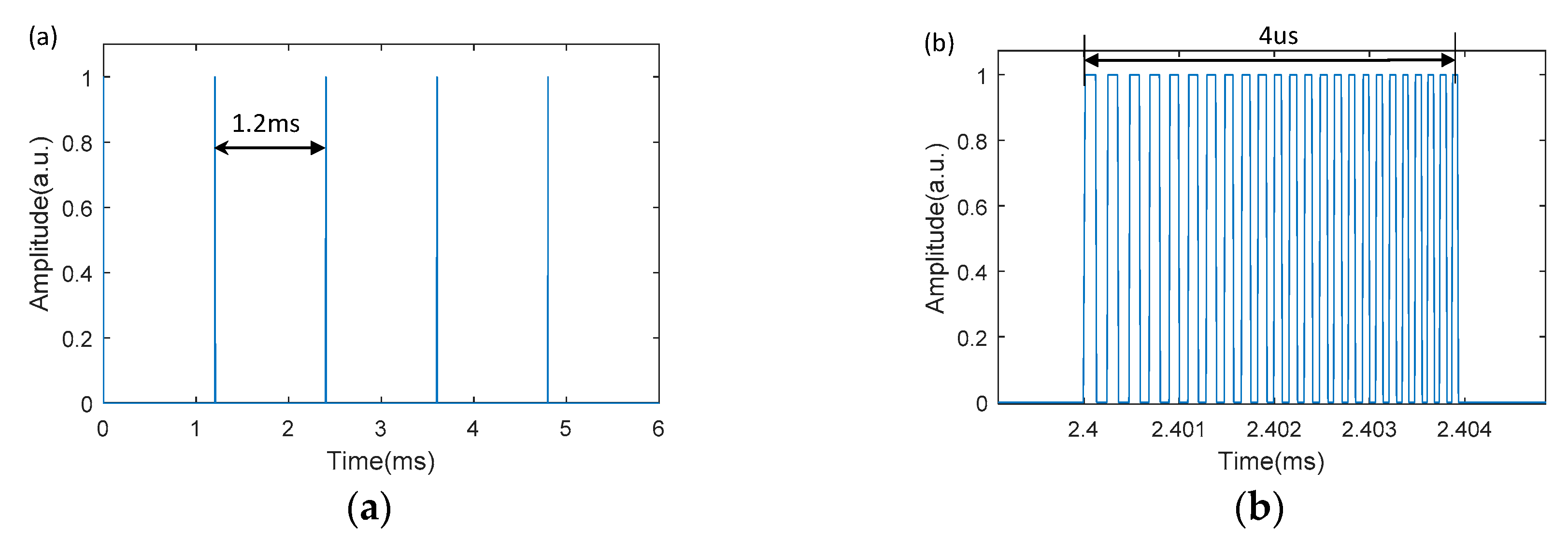
2.1. Digital LFM Signal and Direct Detection

In this section, we introduce a method for generating a digital LFM signal. To clarify the method for generating a digital LFM signal, we need to generate a section of LFM signal S(t) first, expressed as
S ( t ) = r e c t ( t T ) cos ( 2 π f 0 t + π K t 2 ) ,
where T is the pulse width, f0 is the start frequency of the LFM signal, K is the frequency modulation (FM) slope of the LFM signal, and rect(·) denotes the rectangular function.
We propose a digital LFM signal generation method by performing a symbolic operation on S(t). Hence, we can obtain a digital LFM signal DS(t), as follows:
D S ( t ) = r e c t ( t T ) s i g n [ cos ( 2 π f 0 t + π K t 2 ) ] ,
where sign(·) denotes the symbolic operation.
The digital LFM signal represented in Equation (2) is bipolar. However, as shown in Figure 1, we use a direct modulation laser as the optical source at the transmitting end, and the generated signal controls whether the laser is on or off, that is, the optical source can actually produce only a unipolar digital signal representing 0 and 1. With reference to the encoding OTDR, the effect of transmitting bipolar digital signals can be obtained by transmitting two strings of complementary unipolar digital signals. Therefore, the signal generator can emit two series of periodic complementary unipolar digital LFM signals, DSA(t) and DSB(t), expressed as
D S A ( t ) = 1 + D S ( t ) 2 ,   D S B ( t ) = 1 D S ( t ) 2 .
The intensity-modulated optical pulses having DSA(t) and DSB(t) as modulation signals are then sequentially injected into FUT as probe pulses, whose power expressions can be written as
P DSA ( t ) = P 0 · D S A ( t ) ,   P DSB ( t ) = P 0 · D S B ( t ) ,
where P0 is the output optical power of the laser.
As shown in Figure 1, the backscattered light becomes a current signal after the direct detection and photoelectric conversion, and can be expressed as
i D S A ( t ) = R d · P DSA ( t ) G ( t ) ,   i D S B ( t ) = R d · P DSB ( t ) G ( t ) ,
where ⊗ represent a convolution sign, Rd is a constant representing the photodetector responsivity and G(t) is the impulse response of the backscattered light to the probe signal when this is a delta function signal. Finally, the detected signals iDSA(t) and iDSB(t) are differentially operated to recover the bipolar digital LFM signal, as follows:
i s ( t ) = i D S A ( t ) i D S A ( t ) = R d · P 0 · D S ( t ) G ( t ) ,
where the signal is(t) is equivalent to the value measured when the probe signal is bipolar.

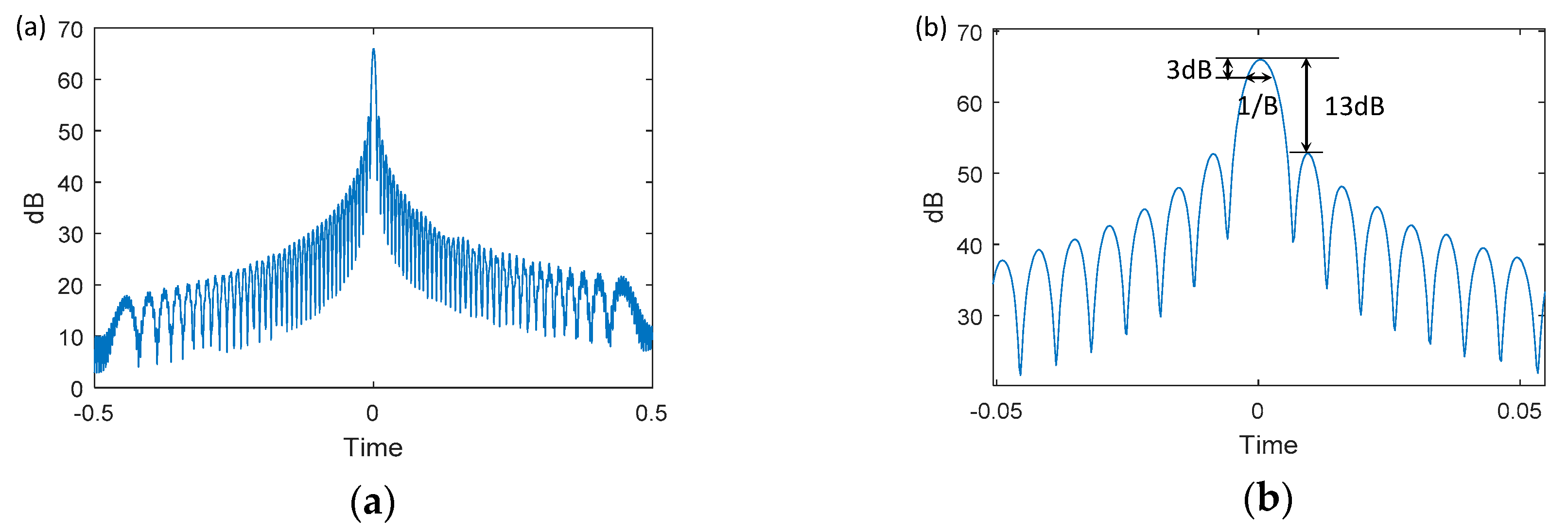
2.2. Short-Time Fractional Fourier Transform

Like the conventional OTDR, DLFM–OTDR also aims to obtain the attenuation characteristics of FUT by detecting the intensity variation of the backscattered signal with the round-trip time. The probe signal used is an intensity-modulated optical pulse whose modulation signal is the electrical digital LFM signal. Therefore, considering how to effectively detect the digital LFM signal in the backscatter signal is very important.
The Fourier series decomposition is performed on Equation (2), which can be rewritten as
D S ( t ) = r e c t ( t T ) [ cos ( 2 π f 0 t + π K t 2 ) 1 3 cos ( 6 π f 0 t + 3 π K t 2 ) + 1 5 cos ( 10 π f 0 t + 5 π K t 2 ) + ] .
Hence, DS(t) can be considered as a linear superposition of various LFM signals, with different FM slopes and start frequencies, which are referred to as primary, tertiary and quinary LFM signals in sequence. Therefore, we only need to effectively extract the LFM signal from the backscattered one.
Figure 2a,b show, respectively, the time-domain waveform and time–frequency distribution of an LFM signal, which has a large time width and bandwidth and is non-stationary, having the frequency changing with time. Thus, the LFM signal can be processed and extracted neither in the time nor frequency domains. The fractional Fourier transform (FrFT) is a generalized Fourier transform that breaks through the traditional way of analysis only in the time, frequency, or time–frequency joint domains [25,26]. It allows the signal analysis in the fractional domain between the time and frequency domains, and all signal characteristics from both domains can be observed [27]. Like the Fourier transform, FrFT is also a base representation method, whose basis function is a set of LFM signals. As shown in Figure 2c, when the FM slope of the selected fractional Fourier domain decomposition is equal to that of the LFM signal, the latter will have an energy aggregation effect on the selected basis [27]. Similar to a narrow bandpass filter in the frequency domain, filtering is performed with a spike in the fractional domain, and with a properly selected bandwidth, the signal energy can be preserved while filtering out most of the noise energy. Therefore, FrFT is very effective in extracting LFM signals and filtering noise.
The effect of filtering can be measured by the signal-to-noise ratio improvement factor IF, which is defined as the ratio of signal-to-noise ratio (SNR) before and after filtering [28],
I F = S N R o u t S N R i n .
If N is defined as the length of the normalized signal sample, the input SNR can be defined as [29]
S N R i n = E [ 0 N 1 | s ( n ) | 2 ] N σ n 2 .
We use a bandpass filter to filter the signal in the fractional domain, and then the output SNR can be estimated as
S N R o u t E [ 0 N 1 | s ( n ) 2 | ] Δ n σ n 2 ,
where Δn is the bandwidth of the narrow bandpass filter on the fractional domain. At this point, the improvement in signal-to-noise ratio is
I F = S N R o u t / S N R i n N / Δ n .
The improvement in SNR is proportional to the length of the signal sample and inversely proportional to the bandwidth of the narrow bandpass filter on the fractional domain.
DLFM–OTDR requires the detection of not only the probe pulse intensity but also its changes over time. STFrFT, a windowed FrFT, is used to detect the strength of an LFM signal of local sections of a signal as it changes over time [23,24]. Therefore, we choose STFrFT as the signal processing method for our proposed DLFM–OTDR. In practice, the procedure for computing STFrFT involves dividing a longer time signal into shorter segments of equal length and successively computing the FrFT separately on each of them.
To clarify the analysis, we first consider how to extract the primary LFM component x(t). The signal x(t) is represented in the complex number to facilitate subsequent mathematical derivation, and is expressed as
x ( t ) = r e c t ( t T ) exp [ j ( 2 π f 0 t + π K t 2 ) ] .
After x(t) is processed by STFrFT, the output signal can be expressed as [22]
S T F R F T x α ( t , u ) = 1 2 π exp [ ( j / 2 ) t 2 cot α ] · + x ( τ ) exp [ ( j / 2 ) τ 2 cot α ] · h * ( t τ ) exp [ j ( t τ ) u csc α ] d τ ,
where α is the FrFT order, -cotα is the FM slope of the fractional Fourier domain decomposition, u is an independent variable in the fractional domain, h(t) is the STFrFT window, and the superscript “*” indicates the conjugate operation. As an example, we choose the simplest rectangular window for STFrFT, expressed as
h ( t ) = r e c t ( t T ) ,
where T is the window length, which is selected as long as the length of the LFM probe pulse.
To achieve energy aggregation of the primary LFM components in the fractional domain, the FM slope of the selected fractional Fourier domain decomposition must be equal to the FM slope of x(t), as follows:
cot α = 2 π K ,
while the relationship between the FrFT independent variables and the Fourier transform independent variables is determined by
f = u csc α 2 π .
By substituting Equations (13–16) into Equation (12) and taking into account the relationship between the frequency f of x(t) and the time t, f = Kt + f0, we can simplify Equation (12) as
S T F R F T s α ( t ) = A 0 2 π exp ( j π K t 2 ) · + r e c t ( t T ) r e c t ( t τ T ) exp [ 2 j π ( K τ + f 0 ) t ] d τ = T A 0 2 π r e c t ( t 2 T ) sin π K ( T | t | ) t π K T t exp ( 2 j π f 0 t ) .
When tT, the envelope of (17) can be approximated as a sinc function, denoted by Sa(·), as follows:
E ( t ) T A 0 2 π r e c t ( t 2 T ) S a ( π K T t ) .
Finally, Equation (6) is substituted into Equation (18) and only the primary LFM components are considered. According to Equation (7), the output expression y(t) of the signal is (t) after STFrFT is
y ( t ) = T P 0 R d 2 π r e c t ( t 2 T ) S a ( π K T t ) G ( t ) .
According to Equations (7) and (19), for other higher-order LFM components, the output result would only differ in the intensity and width of the reflection peak.
According to the characteristics of the sinc function, the 3-dB width or full width at half maximum (FWHM) of the mainlobe of the sinc function is
BW = 2 π t 1 π K T t = 1 K T .
The results of the STFrFT numerical calculation for a section of the LFM pulse based on intensity modulation are shown in Figure 3; the original LFM pulse is compressed into a sinc-shaped narrow pulse by STFrFT. According to Equation (20), the 3 dB width or full width at half maximum (FWHM) of the mainlobe of the sinc function is equal to 1/KT, as shown in Figure 3b. In theory, the DLFM–OTDR spatial resolution is determined by the probe pulse propagation distance in FUT within half time length of the mainlobe FWHM, which can be expressed as
R = c 2 n K T = c 2 n B ,
where c is the speed of light propagation in vacuum, n is the refractive index of FUT, and B = KT is the sweep frequency range of the LFM pulse. Equation (21) shows that the spatial resolution of DLFM–OTDR is determined by the sweep frequency range B and not by the pulse width of the probe pulse. Therefore, our proposed method overcomes the contradiction between the measurement distance and spatial resolution of the conventional OTDR.

2.3. Sidelobe Suppression

When the STFrFT window is rectangular, the output waveform envelope of the LFM pulse processed by STFrFT shows properties similar to those of a sinc function. In addition to the mainlobe, there are a series of sidelobes extending on the time axis. The first sidelobe close to the mainlobe is the largest, with a peak value of 13 dB lower than the mainlobe one, and the peaks of the other sidelobes decrease successively. These sidelobes can overwhelm the signals of some smaller events nearby, resulting in inaccurate measurements. Based on the pulse compression radar, different windows can be used to suppress them [30]. However, suppressing the sidelobes also widens the mainlobe of the output waveform envelope and decreases its peak value, that is, sidelobe suppression comes at the expense of signal-to-noise ratio loss and poor distance resolution. The Hamming window is a sidelobe suppression technique commonly used in pulse compression radars [30], and we used it as an STFrFT window. Figure 4a illustrates the numerical calculation results when using the Hamming window. A comparison between Figure 4a and Figure 3a shows that the peak sidelobe ratio is greatly improved after using the Hamming window, but the mainlobe is widened and its peak value is reduced. In particular, according to the characteristics of the Hamming function, the peak sidelobe ratio can be increased to about 41 dB and the mainlobe can be expanded by 1.47 times [30], as shown in Figure 4b.

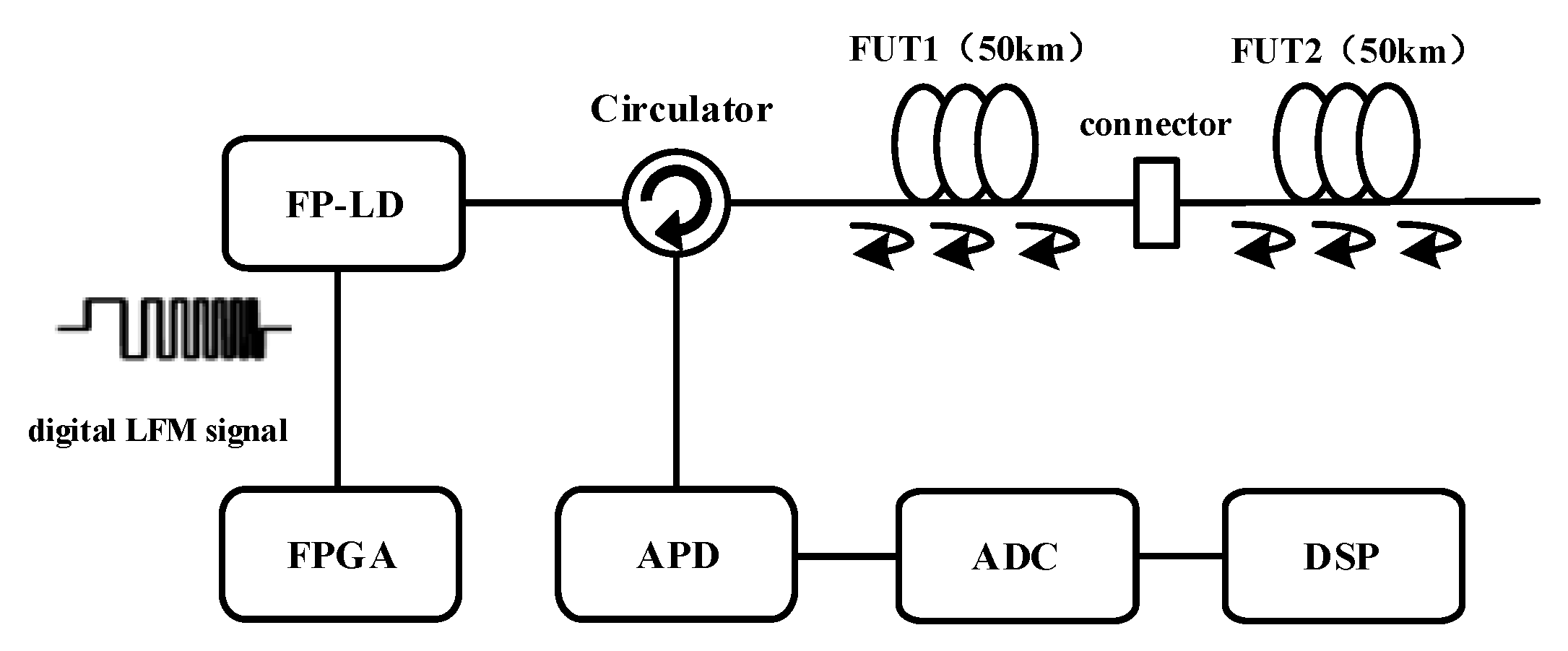
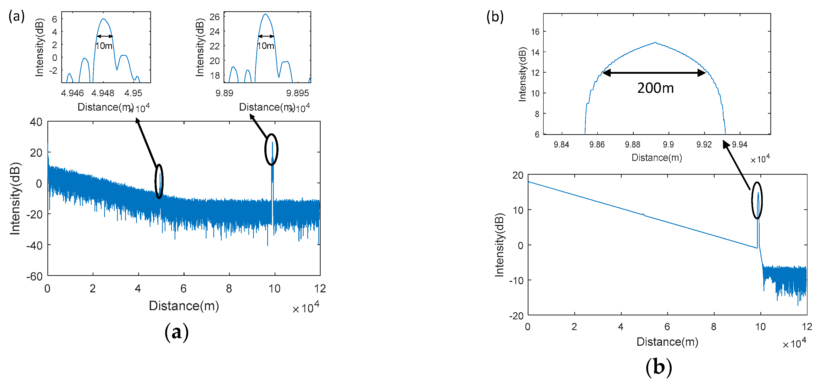
3. Experimental Setup and Results & Discussion

The proof-of-concept experimental system for the proposed DLFM–OTDR is shown in Figure 5. The system is implemented on an existing conventional OTDR development board without any hardware change. A 1625-nm multiple quantum well (MQW) Fabry–Perot (FP) laser diode was used as the optical source, which can only be turned on and off, and it was controlled by a Cyclone V series (Cyclone V 5CGXFC6U19I7N; Altera) field-programmable gate array (FPGA) through a constant current source circuit. The waveform of the digital LFM signal is shown in Figure 6. In order to be able to generate D-LPM pulse sequences on conventional OTDR development board, the conventional OTDR development boards we use are developed by ourselves, and their signal transmission and signal receiving parts are not as good as commercial OTDRs. The bandwidth of the laser driver circuit on the conventional OTDR development board was only 25 MHz. To generate a relatively complete digital LFM signal, its sweep frequency range was only from 4 MHz to 8 MHz (B = 4 MHz), and the pulse width and period were 4 μs and 1.2 ms, respectively. Direct modulation of laser current introduces some spurious phase modulation, in addition to intensity modulation. However, firstly, the pulse signal modulation frequency is from 4 M to 8 M, the modulation frequency is very low, and the generated spurious phase modulation is negligible. Secondly, the receiving end uses intensity detection, which is insensitive to phase modulation. Therefore, the spurious phase modulation has little effect on the system. The backscattered signal was directly detected and converted into a current signal through the avalanche photodiode (APD) (NR8360JP-BC) with a 1 GHz bandwidth. After passing the transimpedance and the signal amplification circuits, the signal was sampled by an analog-to-digital converter (ADC) (AD9230) with a sampling rate of 100 MHz. The STFrFT for the acquired signal was implemented on the computer. For the experiment, two 50-km fibers made up the FUT with a length of 100 km.
The average results of 16384 experiments are shown in Figure 7. By default, the STFrFT window is rectangular. Figure 7a illustrates the measurement result considering only the primary LFM signal in the backscattered signal, showing that the Fresnel reflection event in the FUT can be successfully measured only in this case. Three reflection peaks can be observed. The first and second peaks, respectively at 0 km and 50 km, are caused by the connector. The third peak, at 100 km, is the reflection peak at the fiber end. The spatial resolution, which is the FWHM of the mainlobe of the reflection peak, is 30 m, validating the theoretical spatial resolution of 26 m calculated by substituting n = 1.446 and B = 4 MHz into Equation (21). If a wide-bandwidth laser driver circuit generating a digital LFM signal with a broader sweep frequency range is adopted in DLFM–OTDR, the spatial resolution is expected to be further improved. Note, the fiber attenuation due to the Rayleigh scattering in the fiber cannot be measured when considering only the primary LFM signal. Since the Rayleigh scattering is a random process, the backward Rayleigh scattering signal at the receiver is a superposition of Rayleigh backscattered light at each point in the fiber. Therefore, the power of the backward Rayleigh scattering signal is an average value, which is mainly reflected by the direct current (DC) component of the backscattered signal. The blue curve in Figure 7b represents the measurement result taking into account both the primary LFM signal and the DC component, this DC component is obtained by a digital low-pass filter with a bandwidth of 1 MHz. The blue curve in Figure 7b shows that the simultaneous measurement of the fiber attenuation, and the Fresnel reflection event in the FUT can be achieved by adding a DC component of the backscattered signal. However, the low-pass filter will reduce the signal-to-noise ratio of the reflected signal. What we hope to achieve is to improve its spatial resolution without reducing the dynamic range of the OTDR. The duration of the complementary D-LPM pulse we used was 4 us, so the pulse duration of the single-pulse OTDR is also 4 us. The red curve in the same figure represents the average results of 16384 experiments with a conventional OTDR system having a pulse width of 4 us, under the same experimental conditions. The 400-m spatial resolution of the conventional OTDR is determined by the pulse width, since the pulse width is 4 us and the measurement time is only 19 s and we did not use any other curve fitting technique. The dynamic range of the single-pulse OTDR shown in Figure 7b is less than 20 dB. Figure 7b shows that, under the same conditions, the dynamic range of DLFM–OTDR is improved by 7 dB and the spatial resolution is improved by more than 10 times, compared to the conventional OTDR.
As shown in Figure 7, when the STFrFT window is rectangular, there are a series of evident sidelobes around the high reflection peak in the reflection event measured. To suppress them, we use the Hamming window as the STFrFT window, and the results are shown in Figure 8. Figure 8a illustrates the measurement result when only the primary LFM signal in the backscattered signal is considered. A comparison with the results in Figure 7 suggests that the measured reflection event is mainly a high reflection peak with almost no sidelobes. However, the spatial resolution defined by the FWHM of the mainlobe is reduced by a factor of 1.6 to a width of 48 m, which is almost the same as the result in Figure 4b. Figure 8b shows the measurement results when considering the DC component as well. A comparison with the results in Figure 7b indicates that the dynamic range is still improved by 7 dB with respect to the conventional OTDR and there is no sidelobe in the reflection peak, but this broadens 1.6 times to reach 48 m. Therefore, using the Hamming window as the STFrFT window can significantly suppress the sidelobes in the reflection peaks but also widens the mainlobe.
According to Equation (7), the digital LFM signal can be decomposed into a series of LFM signals with different sweep frequency ranges because the DLFM–OTDR spatial resolution is inversely proportional to the sweep frequency range. The spatial resolution can also be improved without affecting the dynamic range by extracting the higher-order LFM signal with a large sweep frequency range, that is, the tertiary or quinary LFM signal. Figure 9a shows the measurement results obtained by extracting the tertiary LFM signal; since its sweep frequency range is three times that of the primary LFM signal, the spatial resolution is enhanced by 10 times to 10 m. Figure 9b shows the results for the addition of the corresponding DC component; although the dynamic range is not affected, the spatial resolution of the reflection event sharply deteriorates. Since the intensity of the tertiary LFM signal is relatively weak, it is easily covered by the DC component, affecting the spatial resolution of the reflection event.

4. Conclusions

A novel OTDR technique, called DLFM–OTDR, has been proposed. It involves the intensity modulation on the probe pulse, where the modulation signal is the electrical digital LFM signal, and at the receiver, STFrFT is used to process the received signal and filter out noise. We theoretically analyzed and experimentally verified the working principle of DLFM–OTDR. Both the theoretical and experimental results showed that the OTDR spatial resolution is determined by the sweep frequency range of the LFM signal rather than the pulse width. In the demo experiment, a 7-dB improvement in the dynamic range and an approximately 10-times improvement in the spatial resolution were achieved compared to the conventional OTDR. Due to the bandwidth limit of the laser-driver circuit in the conventional OTDR development board, the sweep frequency range of the digital LFM signal ranged only from 4 to 8 MHz (B = 4 MHz). If a wide-bandwidth laser driver circuit generating a digital LFM signal with a broader sweep frequency range is adopted in DLFM–OTDR, the spatial resolution is expected to be further improved. In addition, the influence of the STFrFT window on the peak sidelobe ratio of the reflection peak was studied, proving that the use of a Hamming window can significantly suppress the sidelobes, but at the same time, the mainlobe would be widened by approximately 1.6 times.

Author Contributions

P.Z. finished writing the whole manuscript and conducted experimental verification. Q.F., W.L., Q.Z. and Y.W. presented the idea. P.Z. and Q.F. are the co-first authors.

Funding

This research received no external funding.

Acknowledgments

This work is supported by Open Foundation of China Southern Power Grin and State Key Laboratory of Optical Communication Technologies and Networks (W.R.I.) and the Accelink Technologies Company Ltd.

Conflicts of Interest

The authors declare no conflict of interest.

References

  1. Personick, S.D. Photon probe—An optical-fiber time-domain reflectometer. Bell Syst. Tech. J. 1977, 56, 355–366. [Google Scholar] [CrossRef]
  2. Barnoski, M.K.; Rourke, M.D.; Jensen, S.M.; Melville, R.T. Optical time domain reflectometer. Appl. Opt. 1977, 16, 2375–2379. [Google Scholar] [CrossRef] [PubMed]
  3. Laferriere, J.; Saget, M.; Champavere, A. Original method for analyzing multipaths networks by OTDR measurement. In Proceedings of the Optical Fiber Communication Conference, Dallas, TX, USA, 1997; pp. 99–101. [Google Scholar]
  4. Urban, P.J.; Vall-llosera, G.; Medeiros, E.; Dahlfort, S. Fiber plant manager: An OTDR-and OTM-based PON monitoring system. IEEE Commun. Mag. 2013, 51, S9–S15. [Google Scholar] [CrossRef]
  5. Healey, P.; Booth, R.C.; Daymond-John, B.E.; Nayar, B.K. OTDR in single-mode fibre at 1.5 μm using homodyne detection. Electron. Lett. 1984, 20, 360–362. [Google Scholar] [CrossRef]
  6. Koyamada, Y.; Nakamoto, H. High performance single mode OTDR using coherent detection and fibre amplifiers. Electron. Lett. 1990, 26, 573–575. [Google Scholar] [CrossRef]
  7. Healey, P. Multichannel photon-counting backscatter measurements on monomode fibre. Electron. Lett. 1981, 17, 751–752. [Google Scholar] [CrossRef]
  8. Eraerds, P.; Legre, M.; Zhang, J.; Zbinden, H.; Gisin, N. Photon Counting OTDR: Advantages and Limitations. J. Lightwave Technol. 2010, 28, 952–964. [Google Scholar] [CrossRef] [Green Version]
  9. Nazarathy, M.; Newton, S.A.; Giffard, R.P.; Moberly, D.S.; Sischka, F.; Trutna, W.R.; Foster, S. Real-time long range complementary correlation optical time domain reflectometer. J. Lightwave Technol. 1989, 7, 24–38. [Google Scholar] [CrossRef]
  10. Jones, M.D. Using simplex codes to improve OTDR sensitivity. IEEE Photonics Technol. Lett. 1993, 5, 822–824. [Google Scholar] [CrossRef]
  11. Lee, D.; Yoon, H.; Kim, P.; Park, J.; Kim, N.Y.; Park, N. SNR enhancement of OTDR using biorthogonal codes and generalized inverses. IEEE Photonics Technol. Lett. 2005, 17, 163–165. [Google Scholar]
  12. Izumita, H.; Koyamada, Y.; Furukawa, S.; Sankawa, I. The performance limit of coherent OTDR enhanced with optical fiber amplifiers due to optical nonlinear phenomena. J. Lightwave Technol. 1994, 12, 1230–1238. [Google Scholar] [CrossRef]
  13. Martins, H.F.; Martin-Lopez, S.; Corredera, P.; Salgado, P.; Frazão, O.; González-Herráez, M. Modulation instability-induced fading in phase-sensitive optical time-domain reflectometry. Opt. Lett. 2013, 38, 872–874. [Google Scholar] [CrossRef] [PubMed] [Green Version]
  14. King, J.; Smith, D.; Richards, K.; Timson, P.; Epworth, R.; Wright, S. Development of a coherent OTDR instrument. J. Lightwave Technol. 1987, 5, 616–624. [Google Scholar] [CrossRef]
  15. Healey, P. Fading in heterodyne OTDR. Electron. Lett. 1984, 20, 30–32. [Google Scholar] [CrossRef]
  16. Lee, D.; Yoon, H.; Kim, P.; Park, J.; Park, N. Optimization of SNR improvement in the noncoherent OTDR based on simplex codes. J. Lightwave Technol. 2006, 24, 322–328. [Google Scholar]
  17. Eickhoff, W.; Ulrich, R. Optical frequency domain reflectometry in single-mode fiber. Appl. Phys. Lett. 1981, 39, 693–695. [Google Scholar] [CrossRef]
  18. Bao, X.; Chen, L. Recent progress in distributed fiber optic sensors. Sensors (Basel) 2012, 12, 8601–8639. [Google Scholar] [CrossRef]
  19. Uttam, D.; Culshaw, B. Precision time domain reflectometry in optical fiber systems using a frequency modulated continuous wave ranging technique. J. Lightwave Technol. 1985, 3, 971–977. [Google Scholar] [CrossRef]
  20. Venkatesh, S.; Sorin, W.V. Phase noise considerations in coherent optical FMCW reflectometry. J. Lightwave Technol. 1993, 11, 1694–1700. [Google Scholar] [CrossRef]
  21. Yang, S.; Zou, W.; Long, X.; Chen, J. Pulse-compression optical time domain reflectometer. In Proceedings of the Society of Photo-Optical Instrumentation Engineers Society of Photo-Optical Instrumentation Engineers (SPIE) Conference Series, Santander, Spain, 2 June 2014. [Google Scholar]
  22. Yang, S.; Zou, W.; Long, X.; Chen, J. Optical pulse compression reflectometry: Proposal and proof-of-concept experiment. Opt. Express 2015, 23, 512–522. [Google Scholar]
  23. Tao, R.; Li, Y.-L.; Wang, Y. Short-Time Fractional Fourier Transform and Its Applications. In Proceedings of the IEEE Transactions on Signal Processing, Piscataway, NJ, USA, 14 April 2010; Volume 58, pp. 2568–2580. [Google Scholar]
  24. Aled, T.C.; Williams, D.P. High resolution spectrograms using a component optimized short-term fractional Fourier transform. Signal Process. 2010, 90, 1591–1596. [Google Scholar]
  25. Namias, V. The fractional order Fourier transform and its application to quantum mechanics. J. Inst. Math. Appl. 1980, 25, 241–265. [Google Scholar] [CrossRef]
  26. McBride, A.C.; Kerr, F.H. On Namias’s fractional Fourier transforms. IMA J. Appl. Math. 1987, 39, 159–175. [Google Scholar] [CrossRef]
  27. Almeida, L.B. The fractional Fourier transform and time-frequency representations. IEEE Trans. Signal Process. 1994, 42, 3084–3091. [Google Scholar] [CrossRef]
  28. Sergio, B.; Scaglione, A. Adaptive time-varying cancellation of wideband interferences in spread-spectrum communications based on time-frequency distributions. IEEE Trans. Signal Process. 1999, 47, 957–965. [Google Scholar] [Green Version]
  29. Xia, X.G. A quantitative analysis of SNR in the short-time Fourier transform domain for multicomponent signals. IEEE Trans. Signal Process. 1998, 46, 200–203. [Google Scholar]
  30. Temes, C.L. Sidelobe Suppression in a Range-Channel Pulse-Compression Radar. IRE Trans. Mil. Electron. 1962, 1051, 162–169. [Google Scholar] [CrossRef]
Figure 1. Schematic block diagram of the digital LFM-based optical time-domain reflectometry method. LD: laser diode; APD: avalanche photodiode; FUT: fiber under test; DSP: digital signal processing.
Applsci 09 00668 g001
Figure 2. T-section of an LFM signal (time normalizes with respect to T). (a) Time-domain waveform and (b) time–frequency distribution; (c) fractional Fourier transform when the FM slope of the decomposition basis is equal to that of the LFM signal.
Applsci 09 00668 g002
Figure 3. STFrFT with a rectangular window (time normalizes with respect to T). (a) Compressed narrow pulse of the sinc-shape by STFrFT and (b) zoom-in of the main lobe in (a) with 3-dB width, which is equal to 1/KT, and a peak sidelobe ratio of approximately 13 dB.
Applsci 09 00668 g003
Figure 4. STFrFT with the Hamming window (time normalizes with respect to T). (a) Compressed narrow pulse by STFrFT and (b) zoom-in of the main lobe in (a) with a 3-dB width, which is equal to 1.47/KT, and a peak sidelobe ratio of approximately 41 dB.
Applsci 09 00668 g004
Figure 5. Schematic block diagram of the digital linear frequency modulation (LFM)-based optical time domain reflectometry. FP-LD: Fabry–Perot (FP) laser diode; FPGA: field-programmable gate array; APD: avalanche photodiode; FUT: fiber under test; ADC: analog-to-digital converter; DSP: digital signal processor.
Applsci 09 00668 g005
Figure 6. Periodic digital linear frequency modulation (LFM) signal. (a) Time-domain waveform, with a pulse period of 1.2 ms, (b) zoom-in of the digital LFM signal in (a), with a pulse width of 4 us and a sweep frequency ranging from 4 MHz to 8 MHz (B = 4 MHz).
Applsci 09 00668 g006
Figure 7. Measurement results of the rectangular short-time fractional Fourier transform window. (a) Considering only the primary linear frequency modulation signal in the backscattered signal. (b) The blue curve represents the results obtained when adding the direct current component, and the red curve the results of a conventional optical time domain reflectometry (OTDR) under the same experimental conditions.
Applsci 09 00668 g007
Figure 8. Measurement results of the Hamming short-time fractional Fourier transform window. (a) Considering only the primary linear frequency modulation signal in the backscattered signal and (b) adding the direct current component.
Applsci 09 00668 g008
Figure 9. Measurement results obtained by extracting the tertiary LFM signal. (a) Considering only the tertiary LFM signal in the backscattered signal and (b) adding the direct current component.
Applsci 09 00668 g009

