Article

Three-Dimensional Reconstruction Method for Machined Surface Topography Based on Gray Gradient Constraints

School of Mechanical and Precision Instrument Engineering, Xi’an University of Technology, Xi’an 710048, China
*
Author to whom correspondence should be addressed.
Appl. Sci. 2019, 9(3), 591; https://doi.org/10.3390/app9030591
Submission received: 17 January 2019 / Revised: 1 February 2019 / Accepted: 2 February 2019 / Published: 11 February 2019
(This article belongs to the Section Mechanical Engineering)

Abstract

:

Featured Application

Applying on mechanical engineering.

Abstract

In the modern engineering field, recovering the machined surface topography is important for studying mechanical product function and surface characteristics by using the shape from shading (SFS)-based reconstruction method. However, due to the limitations of many constraints and oversmoothing, the existing SFS-based reconstruction methods are not suitable for machined surface topography. This paper presents a new three-dimensional (3D) reconstruction method of machined surface topography. By combining the basic principle of SFS and the analytic method, the analytic model of a surface gradient is established using the gray gradient as a constraint condition. By efficiently solving the effect of quantization errors and ambiguity of the gray scale on reconstruction accuracy using a wavelet denoising algorithm and image processing technology, the reconstruction algorithm is implemented for machined surface topography. Experimental results on synthetic images and machined surface topography images show that the proposed algorithm can accurately and efficiently recover the 3D shape of machined surface topography.

Graphical Abstract

1. Introduction

Machined surface topography refers to the microgeometry shape left on the workpiece surface by the tools and chips during the process of machining [1], which not only has a significant impact on the function of the mechanical product, but also affects the surface characteristics of the mechanical parts, including wear, lubrication, friction, corrosion resistance, and reflection [2,3,4]. Accurate and effective surface topography information is of importance to the modern engineering field. At present, surface topographic information is mainly obtained by the contact measurement method and non-contact measurement method. The main equipment used in contact measurement method is the stylus profilometer. However, due to the limitations of measurement conditions and stylus, the measurement results of linear sampling points cannot represent the whole surface topography, and the workpiece surface cannot avoid being scratched [5]. Moreover, there are many types of non-contact measurement methods, including optical methods [6], ultrasonic methods [7], and three-dimensional (3D) reconstruction methods. Optical and ultrasonic methods have high requirements for their measurement environment, and they also have a limited measurement range. With the development of 3D reconstruction, 3D reconstruction measurement methods have been widely used for non-contact measurement. Wang et al. [8] proposed the 3D reconstruction method of wear particle surfaces based on a photometric stereo, and obtained the surface topographies of wear particles for further feature-based wear particle identification. Tang et al. [9] used the 3D reconstruction method based on the shape from a focus to determine the grinding wheel surface topography.
Three-dimensional reconstruction is the process of recovering 3D shapes of objects from single or multiple images [10,11,12], and the shape from shading (SFS) method is considered to be one of the fastest and most efficient 3D reconstruction methods [13,14,15]. Therefore, the SFS-based reconstruction method has attracted attention from numerous researchers. Maurer et al. [16] used a method that combined SFS and stereo to establish the functional energy with a detail-preserving anisotropic second-order smoothness term, and estimated the depth of the object surface. Lu et al. [17] proposed a Lambert–Phong hybrid model algorithm, and obtained the coordinate information of the highlighted region of the droplet surface by the mask regions with convolutional neural network (R-CNN). Furthermore, they used the Taylor expansion and Newton iteration method in the reflection model to obtain the heights of all the positions. Sun et al. [18] proposed a new roughness evaluation method based on the complex wavelet enhanced SFS transform, and recovered the 3D topography of a milling surface using the 3D models that were developed from the digital image. Zhu et al. [19] proposed a novel method that uses Fourier transform to fuse the depth from focus (DFF) and SFS, and achieved the reconstruction of the tool wear image in addition to ensuring the continuity of the depth map. Yang et al. [20] used the SFS algorithm to reconstruct the 3D shapes of the welding seam, and extracted the curvature information as the feature vector of the welds from the reconstructed topography. The SFS algorithm is essentially an ill-conditioned problem. Therefore, the SFS algorithm is generally combined with other methods in studies, which adds many constraints when reconstructing the surface topography. However, it easily affects the accuracy and smoothness of the reconstructed surface.
Our analytical model is effective, simple, and easy to use, and has been widely used in the machining field. By using the machining variables such as spindle speed, feed rate, depth of cut, and step over, Ozcelik and Bayramoglu [21] developed a statistical model for surface roughness estimation in a high-speed flat end milling process under wet cutting conditions. Özel and Karpat [22] proposed neural network modeling to predict the surface roughness and tool flank wear over the machining time for a variety of cutting conditions in finish hard turning, and developed regression models to capture process-specific parameters. Based on a constitutive relation of various materials and the mechanics of their cutting process, Ning and Liang [23,24,25] presented an analytical model for predicting temperature distribution in orthogonal machining. Moreover, Ning et al. [26,27,28] also established an analytical modeling of extended chip formation, which can predict the machining forces and calculate the average temperature at the primary shear zone.
For the aforementioned problems, this study proposes a new three-dimensional reconstruction method for effectively and accurately reconstructing the machined surface topography. By combining the basic principle of SFS and the analytic method, the analytic model of the surface gradient is established by using the gray gradient as a constraint condition. The 3D reconstruction algorithm of the machined surface topography is implemented by resolving the effect of quantization errors and ambiguity of gray scale on reconstruction accuracy. This paper will lay a foundation for the online detection of machined surface quality.

2. Reconstruction Principle

2.1. Basic Principle of SFS

The basic idea of SFS is that the illuminated patches of object surfaces correspond to the local regions in the gray image [29]. The gray scale of an image is mainly related to the following four factors: the surface orientation, the illumination direction, the direction of the camera relative to the object surface, and the reflection characteristics of the object surface, as shown in Figure 1.
The normal vectors of surface can be expressed as N (−p, −q, 1), and the function of the object surface is z = f(x, y). Hence, the components of the surface gradient in the x and y direction can be expressed as:
{ p = z / x q = z / y
We assumed that the direction vector of the light source is L(−p0,q0, 1), the intensity of the incident radiance is I0, and the reflection coefficient of the object surface is ρ. θi represents the angle between the normal surface and light source direction. Based on the Lambert reflectance model [30], the reflected radiance Lr can be expressed as follows:
L r = I 0 ρ cos θ i = I 0 ρ p 0 p + q 0 q + 1 p 2 + q 2 + 1 p 0 2 + q 0 2 + 1
It is well-known that the gray scale of the image is proportional to the reflected radiance of the corresponding point on the object surface [31]. Hence, the gray scale of the image E(x, y) that corresponds to surface orientation (p, q) can be expressed as follows:
E ( x , y ) = I 0 ρ 1 + p 0 p + q 0 q 1 + p 2 + q 2 1 + p 0 2 + q 0 2
As shown in the previous equation, the surface orientation has two degrees of freedom, and the gray scale of the image can only provide one constraint. Therefore, the SFS algorithm is essentially an ill-problem, and a unique solution cannot be obtained. Although the constraints and restrictive assumptions can be added, they can only guarantee the smoothness of the solution. Based on the rough characteristics of machined surface topography, the existing SFS algorithm is unable to fulfill the reconstruction requirements.

2.2. Analytic Reconstruction Principle

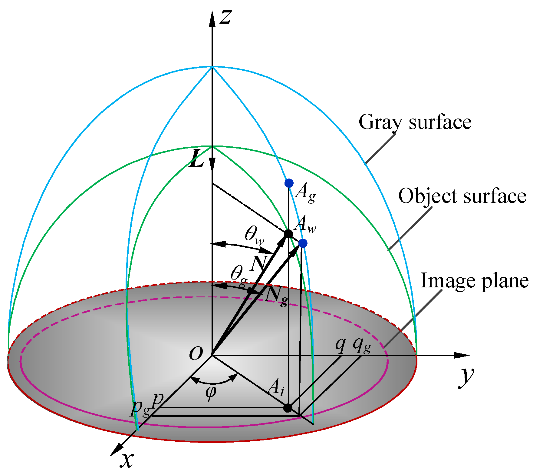
As we mentioned above, the main problem is that conducting an analysis according to the gray scale of image requires the information of the topographical gradient. Furthermore, the gray scale mainly depends on the inclination angle of surface patches. Thus, we propose a reconstruction analytic method to obtain the surface gradient, as shown in Figure 2.
It was supposed that the vector of the light source was L(0, 0, 1), which takes the lens center as the coordinates of the origin. Furthermore, the z-axis of the coordinate system coincides with the optical axis of the imaging system, and the x and y axes are parallel to the imaging plane.
During the process of imaging, the surface topography is projected onto the image plane, and the surface topography data are converted to the gray scale data. The gray surface, which can be used to describe the gray scale distribution of an image, is converted into the object surface. A flatter object surface has a greater gray scale. Ai is a point on the image plane. Ag is the corresponding point on the gray surface with a normal vector of Ng(−pg, −qg, 1) and inclination angle of θg. Aw is the corresponding point on the object surface with a normal vector of N (−p, −q, 1) and inclination angle of θw. φ denotes the declination angle of points.
Based on the analytic geometry theory [32], the declination angle of Ag is equal to that of Aw, both of which are φ. Therefore, the gradient relationship between the object surface and gray surface can be expressed as follows:
p q = p g q g = t g φ
Hence, the object surface gradient can be defined as:
{ p = k p g q = k q g
where k is the gradient scale coefficient. We found that the solution of the SFS algorithm will evolve into a regularization problem by using the gray gradient as the constraint condition.
The gray gradient (pg, qg) is given by the gray scale of image E(x, y):
{ p g = E ( x , y ) x q g = E ( x , y ) y
where E(x, y)x and E(x, y)y represent the gradient of gray scale E(x, y) in the x and y directions, respectively.
Therefore, the object surface gradient can be written as follows:
{ p = k E ( x , y ) x q = k E ( x , y ) y
Furthermore, the vector of the light source L(0, 0, 1) indicates that p0 and q0 are both. By substituting Equation (7) into Equation (3), we obtain an updated formula:
E ( x , y ) = I 0 ρ 1 + k 2 [ E ( x , y ) x 2 + E ( x , y ) y 2 ]
Hence, the gradient scale coefficient is given as:
k ( x , y ) = ± ( ( I 0 ρ ) 2 E ( x , y ) 2 E ( x , y ) 2 [ E ( x , y ) x 2 + E ( x , y ) y 2 ] ) 1 / 2
By substituting Equation (9) into Equation (7), the object surface gradient is expressed as follows:
{ p = ± ( ( I 0 ρ ) 2 E ( x , y ) 2 E ( x , y ) 2 [ E ( x , y ) x 2 + E ( x , y ) y 2 ] ) 1 / 2 E ( x , y ) x q = ± ( ( I 0 ρ ) 2 E ( x , y ) 2 E ( x , y ) 2 [ E ( x , y ) x 2 + E ( x , y ) y 2 ] ) 1 / 2 E ( x , y ) y
Therefore, the surface gradient of each point can be obtained by Equation (10), and the relative height of surface topography can also be calculated by using the integral method.

3. Implementation of Reconstruction Method

Based on the above analytic reconstruction principle, ensuring the accuracy and stability of the gray information of the image is essential in the reconstruction of surface topography. However, machined surface topography has the fractal structure of desertification [33], and the gray scale of the corresponding image easily produces quantization errors and ambiguous information. Hence, it is necessary to solve these two problems and remove their effect on reconstruction accuracy.

3.1. The Quantization Error of Gray Scale

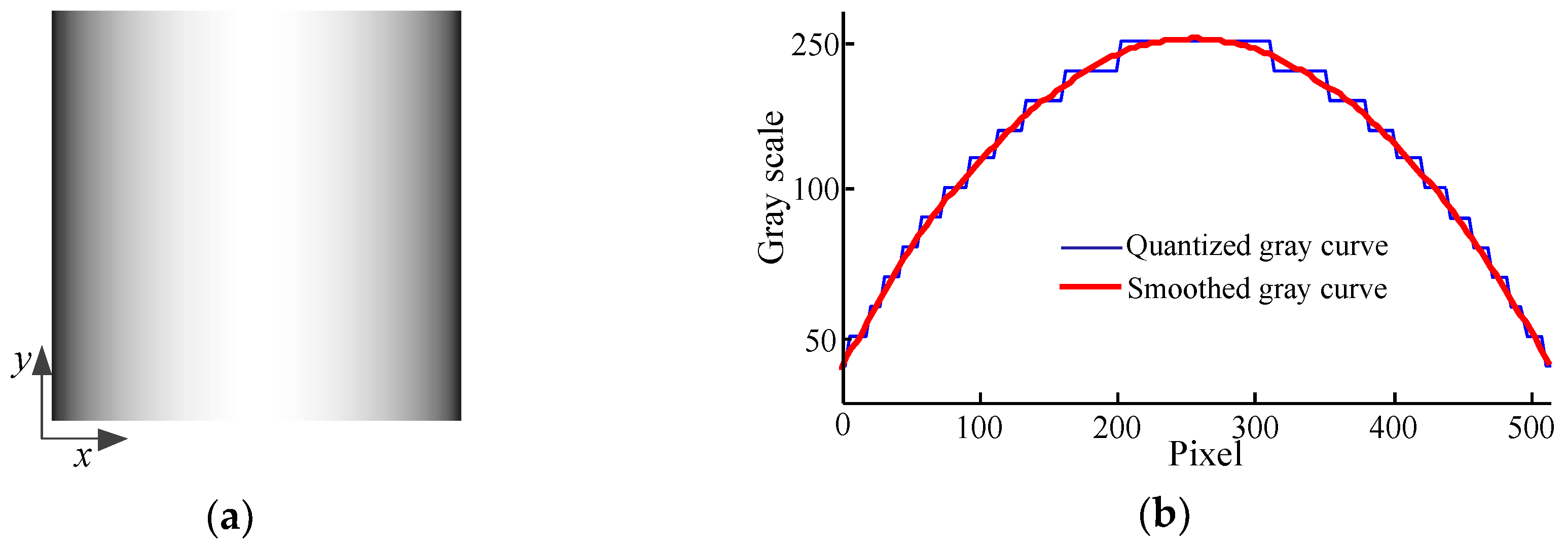
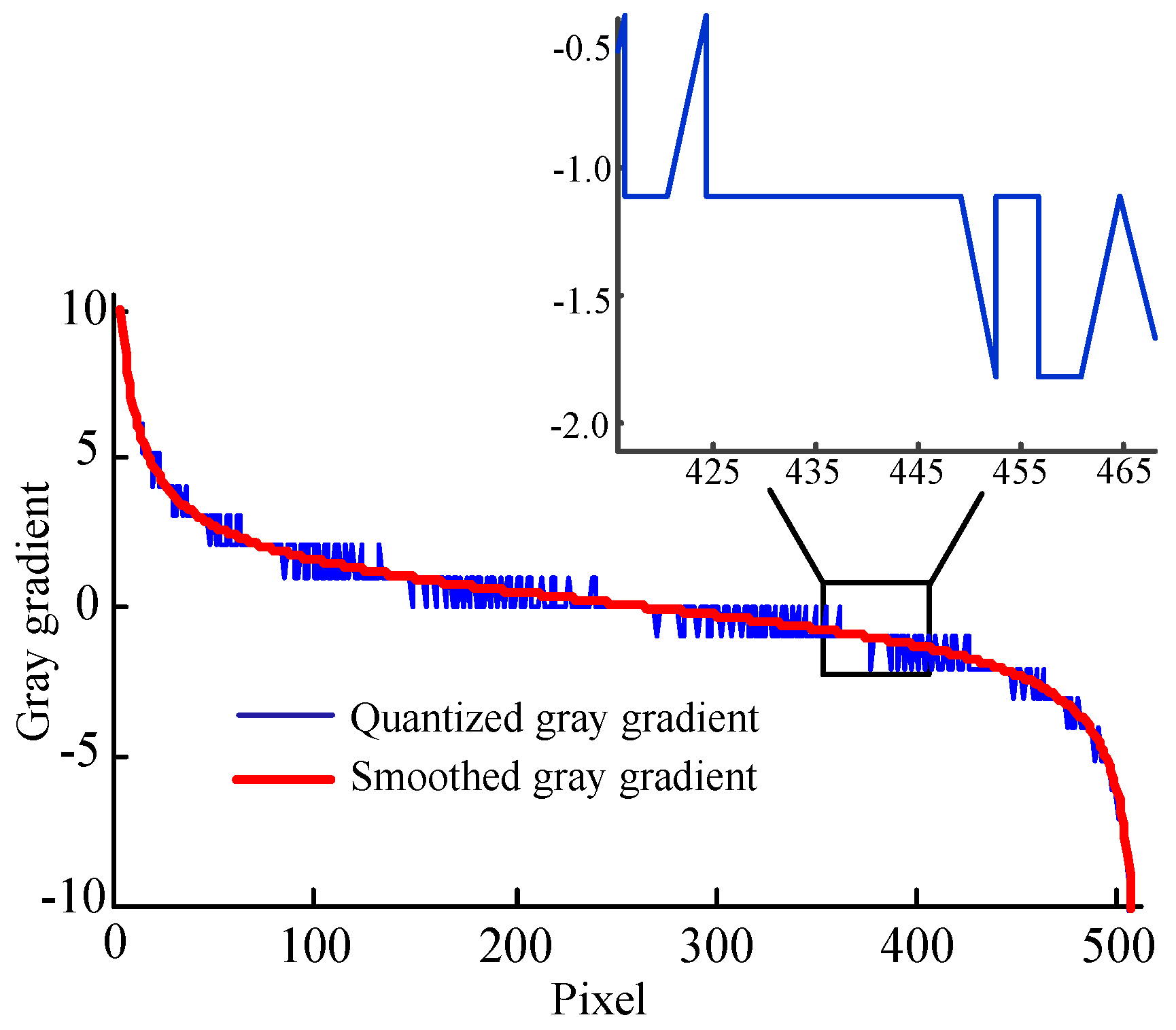
The original image is always obtained by sampling and quantifying the continuously changing gray values [34]. Figure 3 shows the image of a semi-cylindrical surface that satisfies a Lambert reflection model and its gray curve in the x-direction, respectively. It can be seen that the quantized gray values produce random errors with a uniform distribution, and the gray curve presents a discontinuous step-like change. Hence, if the derivative of gray is calculated by using the original image, it will inevitably result in abnormalities in the gray gradient, as shown in Figure 4.
The wavelet denoising algorithm is adopted to eliminate quantization errors [35], which can maintain the details of the gray information and smooth the discontinuity of gray values. By setting an appropriate wavelet decomposition level and quantization threshold for decomposition coefficients, the curves of gray scale and gray gradient were smoothed, as shown in Figure 3b and Figure 4, respectively. It can be seen that the problem of the gray random errors has effectively been solved.

3.2. The Ambiguous Gray Scale

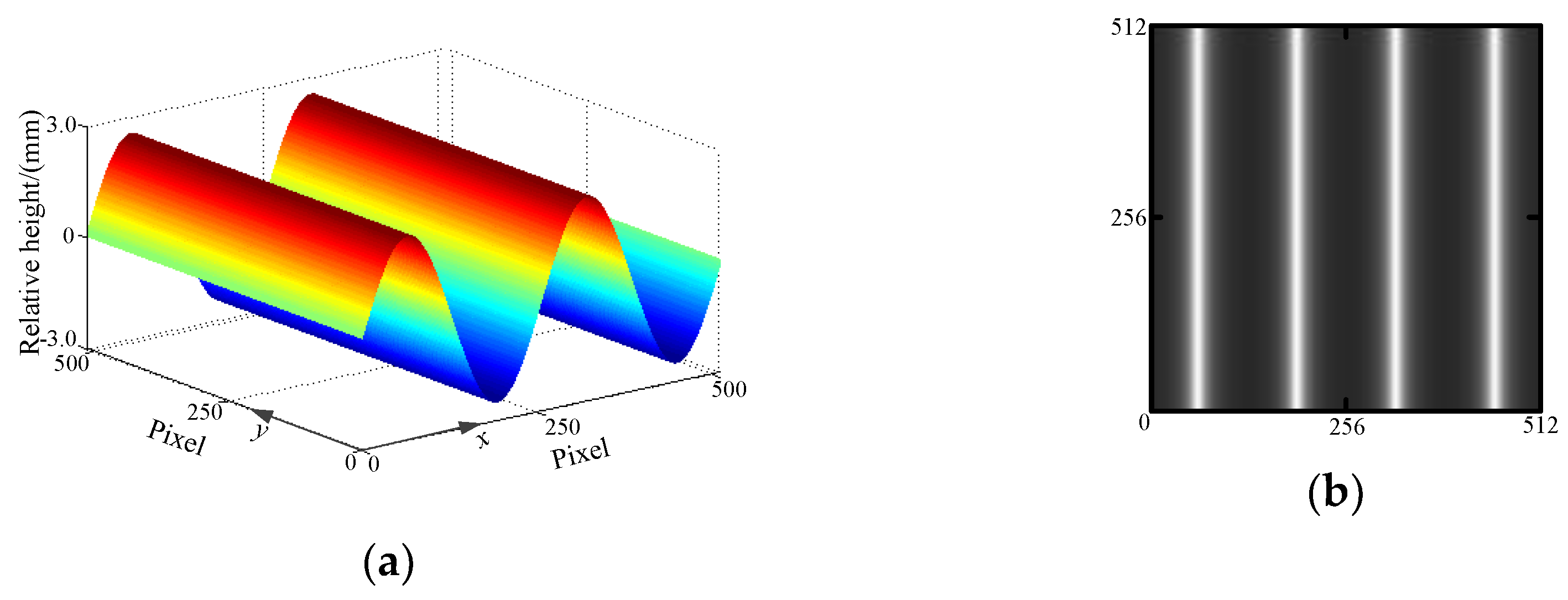
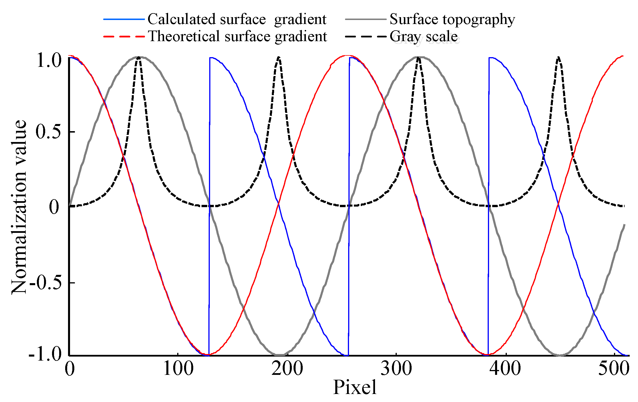
According to Lambert’s reflection theory, the surfaces with an equivalent gradient have the same reflection characteristics. The surface with two peaks and valleys is shown in Figure 5a. The synthetic image of a light source located at (0, 0, 1) is shown in Figure 5b. It can be seen that the gray scales of the peaks are consistent with that of valleys and the peaks. However, the valleys in the surface cannot be distinguished in the synthetic image. Therefore, the image of a surface with multiple peaks and valleys is prone to producing ambiguous gray scale information, resulting in an inability to identify the convexity and concavity of the surface.
The relationship between the topography, gradient, and gray scale of the above-mentioned surface in the x-direction is shown in Figure 6. We can see that the ambiguous gray scale information will mutate the calculated surface gradient, and the mutational points are mainly concentrated in the valleys. Hence, for solving the ambiguous problem of the gray scale, it is important to identify the valley from the image and correct the corresponding calculated surface gradient.
Based on the principle of optical imaging, the points on the focal plane can form a clear image on the imaging sensor, while the image formed by the points outside the focal plane is not clear. Due to the focal plane usually being close to the peaks of surface topography, the images of the peaks are relatively clear. Hence, the clarity of image can be used to identify the peaks and valleys from the image. The image definition represents the clarity of image details and textures [36]. If the image contains richer details, there will be a sharper change in the gray scale that will ultimately produce a clearer image, as shown in Figure 7.
The entropy function evaluation algorithm is an effective evaluation method for image definitions, which calculates the information entropy of an image to evaluate the clarity. The entropy function H(E) can be defined as:
H ( E ) = x = 1 m y = 1 n E ( x , y ) I n [ E ( x , y ) ]
where m × n represents the image size. A larger H(E) will result in a clearer image.
Moreover, the machined surface topography has the statistical self-similarity and self-affinity, as the gray distribution of different rows in the image is similar [37,38]. Therefore, during the process of correcting the surface gradient, each peak value of a gray scale row is first extracted and the sub-images with the same size are collected by taking each peak value as the center. After this, the information entropy of each sub-image is calculated by the entropy function H(E), and the average entropy of all the sub-images is obtained. After this, the sub-image with an information entropy that is lower than the average entropy is defined as the surface valley. Finally, we recognized the column position of the above peak values of the valleys in the image. The gray scales between the minimums on both sides of the column are extracted, and the corresponding calculated surface gradient values are corrected.

3.3. Reconstruction Algorithm

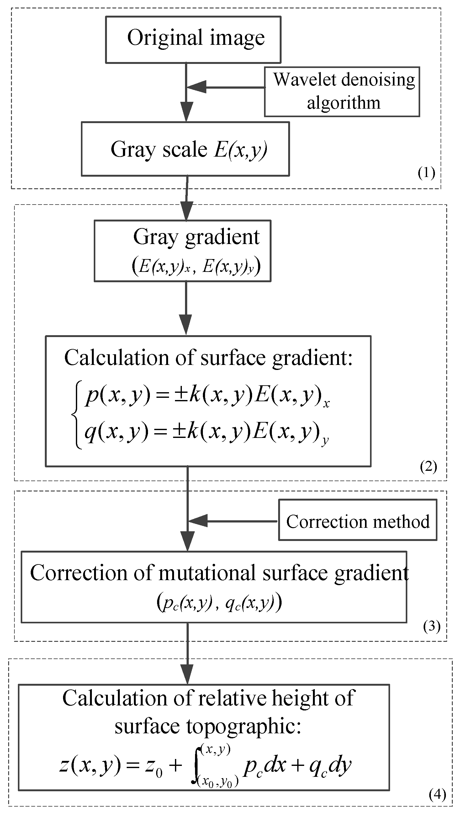
Based on the above-mentioned points, a schematic of the reconstruction algorithm is presented, which is shown in Figure 8. The algorithm mainly consists of four procedures: denoising and smoothing of the original image, analytic calculation of the surface gradient, correction of the mutational surface gradient, and calculation of the topographic relative height.
(1) We read the data of the original image. The gray scale E(x, y) can be obtained without quantization errors by using the wavelet denoising algorithm.
(2) Based on the gray scale E(x, y), the gray gradient (Ex, Ey) can be obtained by the following equation:
{ E ( x , y ) x = ( E ( x + 1 , y ) E ( x 1 , y ) ) / 2 E ( x , y ) y = ( E ( x , y + 1 ) E ( x , y 1 ) ) / 2
Moreover, the surface gradient corresponding to the gray scale E(x, y) of each point in the image is calculated by Equation (10).
(3) The mutational points are found, and their corresponding calculated surface gradients are corrected by adopting the above-mentioned correction method.
(4) We assumed that z0 is the height of the reference point (x0, y0) in the image, and subsequently set the height of the reference point. Thus, the relative height of any point on the object surface can be calculated as follows:
z ( x , y ) = z 0 + ( x 0 , y 0 ) ( x , y ) p c d x + q c d y

4. Experiments

To verify the effectiveness and accuracy of the proposed reconstruction algorithm, we have conducted several experiments on both synthetic images and machined surface topography images. The image and data processing is performed on a PC with AMD Ryzen processors. The proposed reconstruction algorithm is implemented using MATLAB codes.

4.1. Experimental Results on Synthetic Images

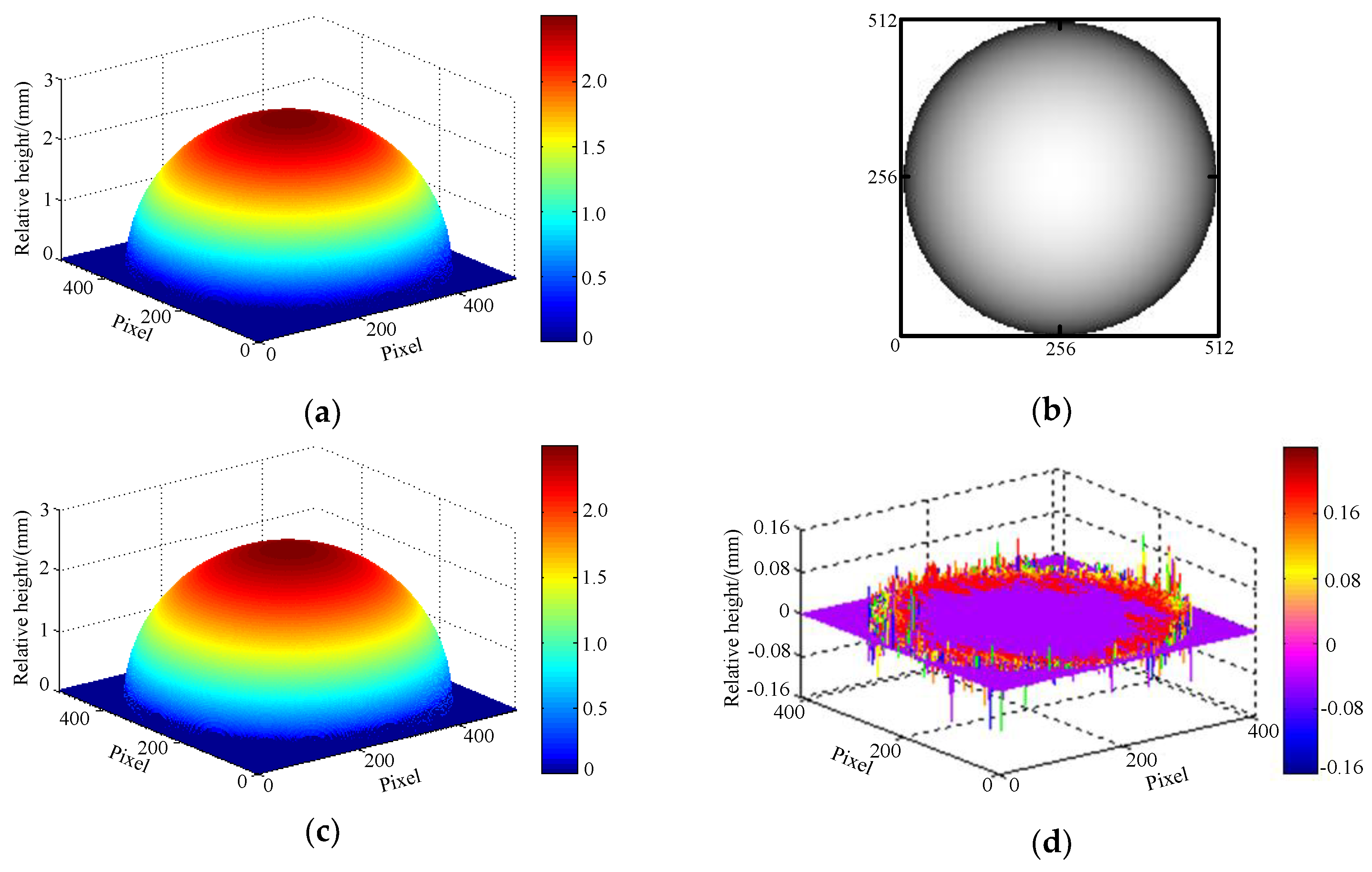
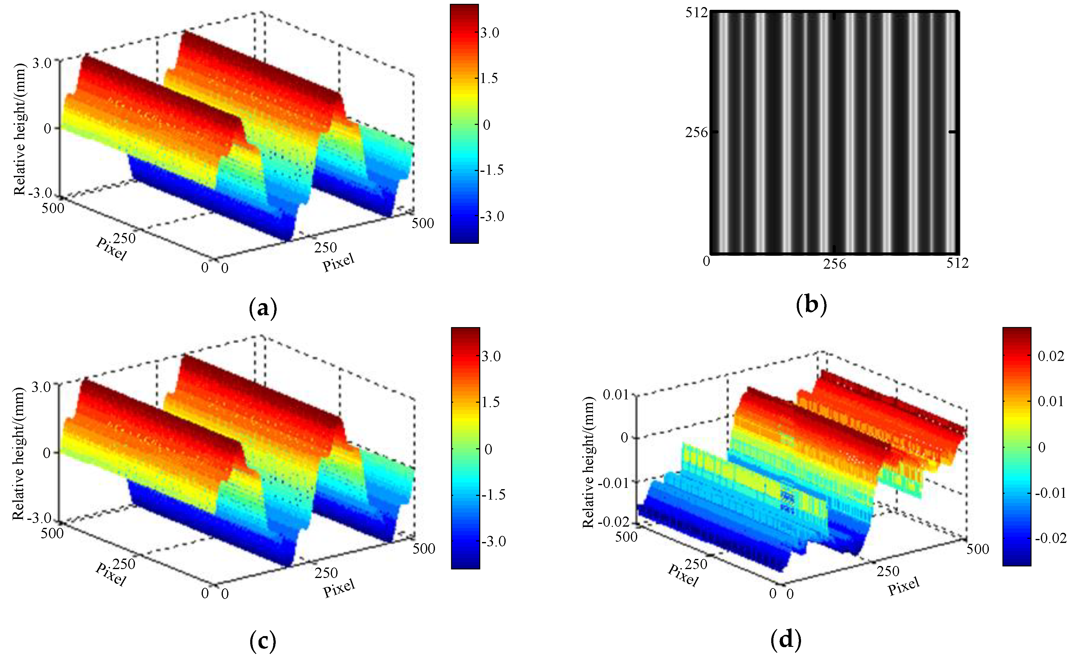
The experiments employ the images of a semi-spherical surface and sinusoidal surface, which are the benchmark images in some studies [39,40]. The semi-spherical and sinusoidal surfaces are generated by the surface formula, which is shown in Figure 9a and Figure 10a, respectively. The diameter of the semi-spherical is five mm. The amplitudes of the sinusoidal surface are 2.5 mm and 0.5 mm, respectively, and the frequency difference is five times. The two synthetic images are formed by the Lambert model, where the vector of the light source is (0, 0, 1).
Figure 9b and Figure 10b illustrate the synthetic images of the two original surfaces, while the reconstructed surfaces are shown in Figure 9c and Figure 10c, respectively. Figure 9d and Figure 10d show the errors between the original surfaces and reconstructed surfaces. It can be seen that the reconstructed surfaces are similar to the original surfaces, with the maximum error values being less than 0.154 mm and 0.0178 mm, respectively. The reconstruction errors mainly occur near the boundary, while the errors of the other points are negligible. This is due to the discontinuity of the boundary surface resulting in the abnormal change in the gray scale. At the same time, it is apparent from the figure that although there is ambiguous gray-scale information in the synthetic image, the peaks and valleys of the surface can be accurately recovered using the proposed correction method.
To evaluate the performance of the proposed reconstruction algorithm, the comparison of the original surface and the reconstructed surface is studied using the mean absolute error (MAE) and root mean square error (RMSE). The results are shown in Table 1.
As shown in Table 2, the MAE between the reconstruction surface and the original surface is small, and the maximum RMSE is only 0.982. It indicates that the reconstructed surfaces are consistent with the original surfaces. The verification results show that the proposed reconstruction algorithm performs well and has high accuracy.

4.2. Experimental Results on Machined Surface Topography Image

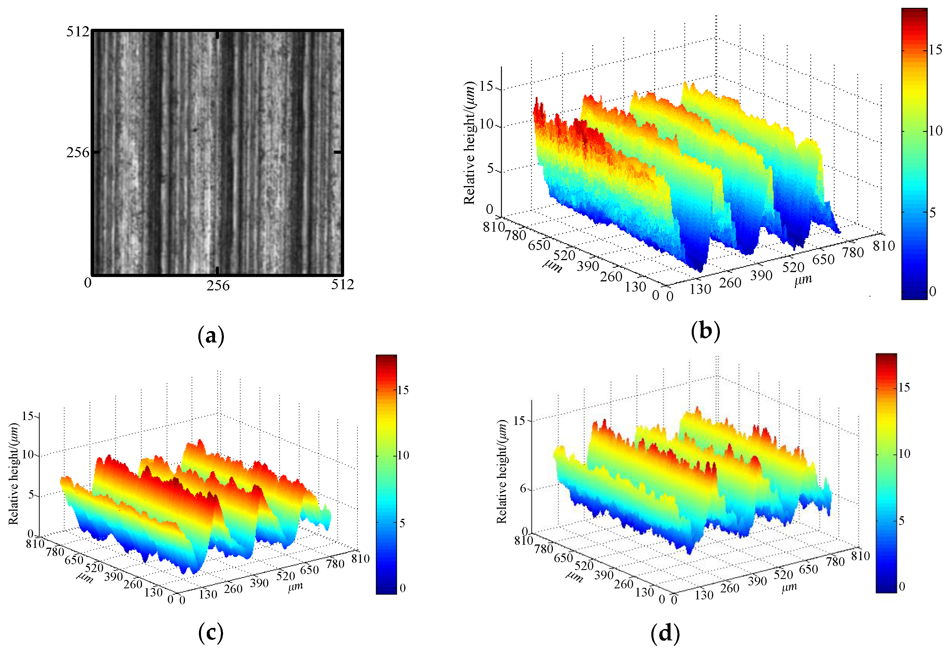
Machining surfaces from turning, milling, and boring operations were recovered using the presented algorithm for the investigation of effectiveness. By using a Leica DCM 3D white light confocal interference microscope, the images for reconstruction containing 512 × 512 pixels are collected, and the corresponding topographic data are measured. Moreover, the reconstruction results are compared with that of the existing SFS algorithm of Horn and Brooks. Figure 11, Figure 12 and Figure 13 show the measured results and reconstruction results of machined surface topography, respectively.
From the above-mentioned reconstruction results, it can be seen that some peaks of the reconstructed surface contain distorted topography. This is due to the effect of light or impurities created during the imaging process, resulting in abnormal gray scales in the image. This is shown in the red boxes in Figure 12a. Figure 11c, Figure 12c, and Figure 13c show the surface topography recovered by the Horn and Brooks algorithm. We can see that a considerable number of detailed features are lost, which means that we cannot clearly show the texture and undulation of the surface. Furthermore, the heights of the reconstruction surface are higher. It is mainly caused by the algorithm, including the excessive smooth constraints. Moreover, we can see that the whole undulation of topography recovered by the proposed algorithm is basically the same as that of the measured results. The reconstruction surface details are abundant, and the reconstruction effect is much better than that of the Horn and Brooks algorithm, as shown in Figure 11d, Figure 12d, and Figure 13d.
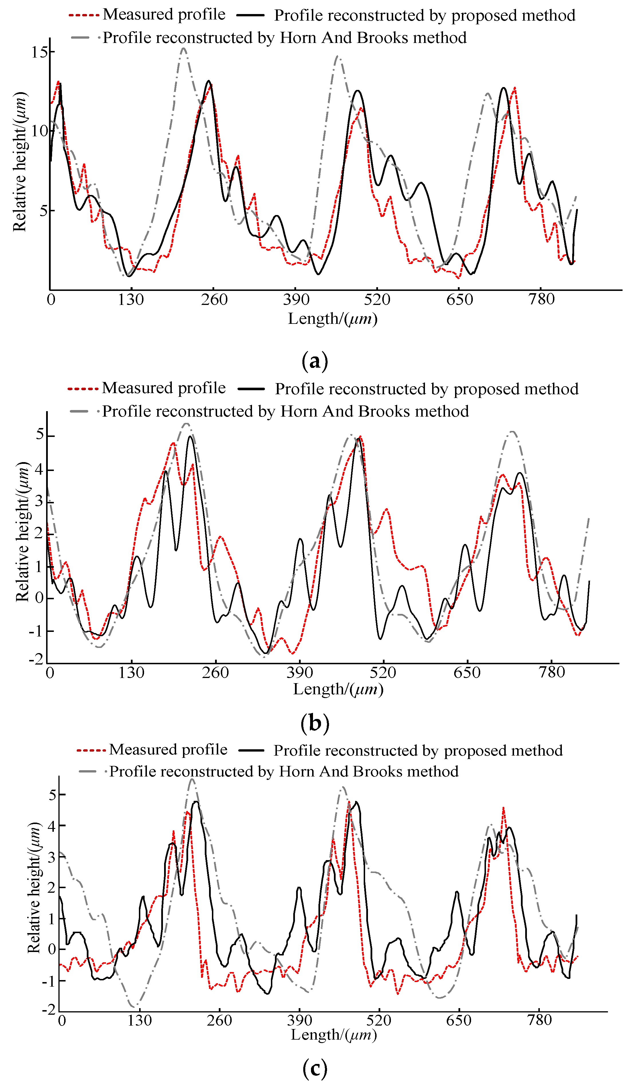
We extracted the profiles of the same position from the above-mentioned topography and the profile between the reconstructed topography and measured topography, which were compared. The results are shown in Figure 14.
It can be seen that the profiles reconstructed by the Horn and Brooks algorithm are different to the measured profile, and the deviations between them are larger. Hence, the reconstruction method based on the Horn and Brooks algorithm is not suitable for machined surface topography. On the contrary, the spacing and height of peaks and valleys between the profiles that were reconstructed by the proposed method and measured profiles are similar. Due to the interference of mutual reflection, secondary reflection, noise, or stray radiation, which are inevitable in the imaging process, the results in some details of the profiles are different. However, from the distribution of peaks and valleys, the profiles reconstructed by the proposed method are very close to the measured profile.
The arithmetic average roughness (Ra), maximum height of the profiles (Rz), and root mean square roughness (Rq) are used to compare the profile reconstructed by the proposed method and measured profile. The results are shown in Table 2.
As shown in Table 2, the relative error between the reconstructed profile and the measured profile is small: less than 10%. It indicates that the reconstructed data are very close to the measured data, and the reconstruction accuracy can meet the requirements of surface topography measurements. Therefore, the experimental results demonstrate that the proposed algorithm can accurately and effectively reconstruct the machined surface topography.

5. Conclusions

(1) Based on the basic principle of the SFS algorithm combined with the analytic method, a new three-dimensional (3D) reconstruction method is introduced to recover machined surface topography. By using the gray gradient as the constraint condition, the relationship between the surface gradient and gray gradient is described, and the analytic model of the surface gradient is developed. Moreover, the problem of SFS can evolve into a regularization problem using the proposed reconstruction principle.
(2) The quantization error and ambiguity of the gray scale has a significant influence on the reconstruction accuracy of machined surface topography. Hence, we apply the wavelet denoising algorithm and the image processing technology to effectively solve those problems, and develop the 3D reconstruction algorithm for machined surface topography.
(3) Experimental results on synthetic images and machined surface topography images reveal that the proposed algorithm is effective, and the profiles of the reconstructed topography are very close to the measured profiles with a relative error of less than 10%.
(4) The proposed three-dimensional reconstruction method solves the problem of accuracy and smoothness of the reconstructed surface. However, there must be a “more or less” limitation that the geometric features of specimen surface topography are relatively good. Hence, it is quite valuable to extend the measured surface.

Author Contributions

Conceptualization, W.-C.S. and J.-M.Z.; methodology, W.-C.S.; software, X.-B.L.; validation, W.-C.S., J.-M.Z. and Y.L.; formal analysis, W.-C.S.; investigation, W.-C.S.; resources, W.-C.S.; data curation, W.-C.S.; writing—original draft preparation, W.-C.S.; writing—review and editing, W.-C.S.; supervision, Y.L.; project administration, J.-M.Z.; funding acquisition, J.-M.Z.

Funding

This research was funded by Natural Science Foundation Research Project of Shaanxi Province (51575237).

Acknowledgments

Thank the Shaanxi Provincial Natural Science Foundation. Thanks to Jianming Zheng for guiding the article. Thanks to other authors for their help with the article.

Conflicts of Interest

The authors declare no conflict of interest.

References

  1. Zhang, X.; Zhang, W.; Zhang, J.; Pang, B.; Zhao, W. Systematic study of the prediction methods for machined surface topography and form error during milling process with flat-end cutter. Proc. Inst. Mech. Eng. Part B J. Eng. Manuf. 2017, 233, 226–242. [Google Scholar] [CrossRef]
  2. Krolczyk, G.M.; Maruda, R.W.; Krolczyk, J.B.; Nieslony, P.; Wojciechowski, S.; Legutko, S. Parametric and nonparametric description of the surface topography in the dry and MQCL cutting conditions. Measurement 2018, 121, 225–239. [Google Scholar] [CrossRef]
  3. Lesyk, D.A.; Martinez, S.; Mordyuk, B.N.; Dzhemelinskyi, V.V.; Lamikiz, A.; Prokopenko, G.I. Effects of laser heat treatment combined with ultrasonic impact treatment on the surface topography and hardness of carbon steel AISI 1045. Opt. Laser Technol. 2019, 111, 424–438. [Google Scholar] [CrossRef]
  4. Grobelny, P.; Furmanski, L.; Legutko, S. Investigations of Surface Topography of Hot Working Tool Steel Manufactured with the Use of 3D Print. MATEC Web Conf. 2017, 137, 02004. [Google Scholar] [CrossRef] [Green Version]
  5. Launhardt, M.; Wörz, A.; Loderer, A.; Laumer, T.; Drummer, D.; Hausotte, T.; Schmidt, M. Detecting surface roughness on SLS parts with various measuring techniques. Polym. Test. 2016, 53, 217–226. [Google Scholar] [CrossRef]
  6. Do Vale, J.L.; de Beltrão, V.C.; da Silva, C.H.; Pintaúde, G. Evaluation of the error of the light beam incidence on concave surfaces in 3D roughness parameters using optical interferometry. Measurement 2018, 120, 182–192. [Google Scholar] [CrossRef]
  7. Srivastava, M.; Hloch, S.; Krejci, L.; Chattopadhyaya, S.; Dixit, A.R.; Foldyna, J. Residual stress and surface properties of stainless steel welded joints induced by ultrasonic pulsed water jet peening. Measurement 2018, 127, 453–462. [Google Scholar] [CrossRef]
  8. Wang, S.; Wu, T.; Yang, L.; Kwok, N.; Sarkodie-Gyan, T. Three-dimensional reconstruction of wear particle surface based on photometric stereo. Measurement 2019, 133, 350–360. [Google Scholar] [CrossRef]
  9. Tang, J.; Qiu, Z.; Li, T. A novel measurement method and application for grinding wheel surface topography based on shape from focus. Measurement 2019, 133, 495–507. [Google Scholar] [CrossRef]
  10. Tang, S.; Zhang, X.; Song, Z.; Jiang, H.; Nie, L. Three-dimensional surface reconstruction via a robust binary shape-coded structured light method. Opt. Eng. 2017, 56, 014102. [Google Scholar] [CrossRef] [Green Version]
  11. Zhou, D.S.; Wang, R.; Lu, J.; Zhang, Q. Depth Image Super Resolution Based on Edge-Guided Method. Appl. Sci. 2018, 8, 298. [Google Scholar] [CrossRef]
  12. Jia, C.L.; Mi, S.B.; Barthel, J.; Wang, D.W.; Dunin-Borkowski, R.E.; Urban, K.W.; Thust, A. Determination of the 3D shape of a nanoscale crystal with atomic resolution from a single image. Nat. Mater. 2014, 13, 1044–1049. [Google Scholar] [CrossRef] [PubMed]
  13. Hu, J.-F.; Zheng, W.-S.; Xie, X.; Lai, J. Sparse transfer for facial shape-from-shading. Pattern Recognit. 2017, 68, 272–285. [Google Scholar] [CrossRef]
  14. Ma, L.; Lyu, Y.; Pei, X.; Hu, Y.M.; Sun, F.M. Scaled SFS method for Lambertian surface 3D measurement under point source lighting. Opt. Express 2018, 26, 14251. [Google Scholar] [CrossRef] [PubMed]
  15. Heise, B.; Stifter, D. Quantitative phase reconstruction for orthogonal-scanning differential phase-contrast optical coherence tomography. Opt. Lett. 2009, 34, 1306. [Google Scholar] [CrossRef] [PubMed]
  16. Maurer, D.; Ju, Y.C.; Breuß, M.; Bruhn, A. Combining shape from shading and stereo: A Joint variational method for estimating depth, illumination and albedo. Int. J. Comput. Vis. 2018, 126, 1342–1366. [Google Scholar] [CrossRef]
  17. Lu, S.; Ren, C.; Zhang, J.; Zhai, Q.; Liu, W. A novel approach to droplet’s 3D shape recovery based on mask R-CNN and improved Lambert–Phong model. Micromachines 2018, 9, 462. [Google Scholar] [CrossRef] [PubMed]
  18. Sun, W.; Chen, B.; Yao, B.; Cao, X.; Feng, W. Complex wavelet enhanced shape from shading transform for estimating surface roughness of milled mechanical components. J. Mech. Sci. Technol. 2017, 31, 823–833. [Google Scholar] [CrossRef]
  19. Zhu, A.; He, D.; Zhao, J.; Luo, W.; Chen, W. 3D Wear area reconstruction of grinding wheel by frequency-domain fusion. Int. J. Adv. Manuf. Technol. 2016, 88, 1111–1117. [Google Scholar] [CrossRef]
  20. Yang, L.; Li, E.; Long, T.; Fan, J.; Mao, Y.; Fang, Z.; Liang, Z. A welding quality detection method for arc welding robot based on 3D reconstruction with SFS algorithm. Int. J. Adv. Manuf. Technol. 2017, 94, 1209–1220. [Google Scholar] [CrossRef]
  21. Ozcelik, B.; Bayramoglu, M. The statistical modeling of surface roughness in high-speed flat end milling. Int. J. Mach. Tools Manuf. 2006, 46, 1395–1402. [Google Scholar] [CrossRef]
  22. Özel, T.; Karpat, Y. Predictive modeling of surface roughness and tool wear in hard turning using regression and neural networks. Int. J. Mach. Tools Manuf. 2005, 45, 467–479. [Google Scholar] [CrossRef]
  23. Ning, J.; Liang, S. Prediction of Temperature Distribution in Orthogonal Machining Based on the Mechanics of the Cutting Process Using a Constitutive Model. J. Manuf. Mater. Process. 2018, 2, 37. [Google Scholar] [CrossRef]
  24. Ning, J.; Liang, S. Predictive Modeling of Machining Temperatures with Force–Temperature Correlation Using Cutting Mechanics and Constitutive Relation. Materials 2019, 12, 284. [Google Scholar] [CrossRef] [PubMed]
  25. Ning, J.; Liang, S. Evaluation of an Analytical Model in the Prediction of Machining Temperature of AISI 1045 Steel and AISI 4340 Steel. J. Manuf. Mater. Process. 2018, 2, 74. [Google Scholar] [CrossRef]
  26. Ning, J.; Nguyen, V.; Liang, S.Y. Analytical modeling of machining forces of ultra-fine-grained titanium. Int. J. Adv. Manuf. Technol. 2018, 99, 1131–1140. [Google Scholar] [CrossRef]
  27. Ning, J.; Liang, S.Y. Model-driven determination of Johnson-Cook material constants using temperature and force measurements. Int. J. Adv. Manuf. Technol. 2018, 97, 1053–1060. [Google Scholar] [CrossRef]
  28. Ning, J.; Nguyen, V.; Huang, Y.; Hartwig, K.T.; Liang, S.Y. Inverse determination of Johnson–Cook model constants of ultra-fine-grained titanium based on chip formation model and iterative gradient search. Int. J. Adv. Manuf. Technol. 2018, 99, 1131–1140. [Google Scholar] [CrossRef]
  29. Tozza, S.; Falcone, M. Analysis and approximation of some shape-from-shading models for non-Lambertian surfaces. J. Math. Imaging Vis. 2016, 55, 153–178. [Google Scholar] [CrossRef]
  30. Alhulayil, M.; Younes, A.B.; Turner, J.D. Higher order algorithm for solving lambert’s problem. J. Astronaut. Sci. 2018, 65, 400–422. [Google Scholar] [CrossRef]
  31. Wang, G.; Cheng, J. Three-dimensional reconstruction of hybrid surfaces using perspective shape from shading. Optik 2016, 127, 7740–7751. [Google Scholar] [CrossRef]
  32. Lv, L.G. Vectors and coordinates. In Analytic Geometry; Higher Education Press: Beijing, China, 2011. [Google Scholar]
  33. Shi, W.C.; Zheng, J.M.; Li, Y.; Li, X.B.; An, Q.N. Measurement and modeling of bidirectional reflectance distribution function (BRDF) on cutting surface based on the coaxial optical microscopic imaging. Optik 2018, 170, 278–286. [Google Scholar] [CrossRef]
  34. Meng, Q.; Wang, H.; Xu, W.; Zhang, Q. A coupling method incorporating digital image processing and discrete element method for modeling of geomaterials. Eng. Comput. 2018, 35, 411–431. [Google Scholar] [CrossRef]
  35. Xu, J.; Wang, Z.; Tan, C.; Si, L.; Zhang, L.; Liu, X. Adaptive Wavelet Threshold Denoising Method for Machinery Sound Based on Improved Fruit Fly Optimization Algorithm. Appl. Sci. 2016, 6, 199. [Google Scholar] [CrossRef]
  36. Yi, H.A.; Liu, J.; Lu, E.H. Detection Method of Grinding Surface Roughness Based on Image Definition Evaluation. J. Mech. Eng. 2016, 52, 15–21. [Google Scholar] [CrossRef]
  37. Izquierdo, S.; López, C.I.; Valdés, J.R.; Miana, M.; Martínez, F.J.; Jiménez, M.A. Multiscale characterization of computational rough surfaces and their wear using self-affine principal profiles. Wear 2012, 274–275, 1–7. [Google Scholar] [CrossRef]
  38. Grzemba, B.; Pohrt, R.; Teidelt, E.; Popov, V.L. Maximum micro-slip in tangential contact of randomly rough self-affine surfaces. Wear 2014, 309, 256–258. [Google Scholar] [CrossRef]
  39. Bruvoll, S.; Reimers, M. Spherical surface parameterization for perspective shape from shading. Pattern Recognit. Lett. 2012, 33, 33–40. [Google Scholar] [CrossRef]
  40. Yang, L.; Zhang, N.; Ren, Y.; Hu, H. Linear perspective shape-from-shading method with two images. J. Syst. Eng. Electron. 2015, 26, 1080–1087. [Google Scholar] [CrossRef]
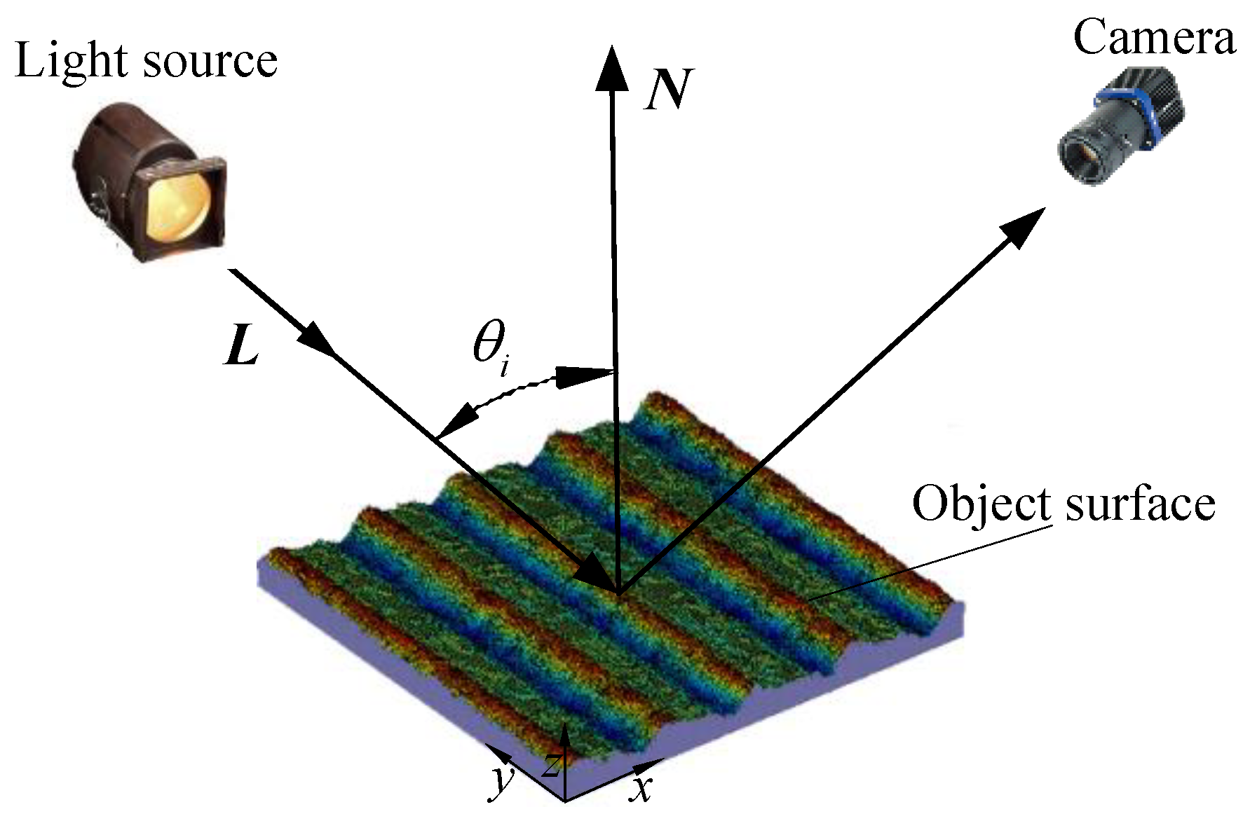
Figure 1. Shape from shading (SFS) model.
Applsci 09 00591 g001
Figure 2. Analytic reconstruction principle.
Applsci 09 00591 g002
Figure 3. (a) Semi-cylindrical image; and (b) Gray curve in the x-direction.
Applsci 09 00591 g003
Figure 4. Gray gradient curve in the x-direction.
Applsci 09 00591 g004
Figure 5. (a) Multiple peaks and surface valleys; and (b) Synthetic image.
Applsci 09 00591 g005
Figure 6. The relationship between surface topography, surface gradient, and gray scale.
Applsci 09 00591 g006
Figure 7. The change in gray scale: (a) Clear image; and (b) Blurred image.
Applsci 09 00591 g007
Figure 8. Analytic reconstruction algorithm.
Applsci 09 00591 g008
Figure 9. Simulation results of the semi-spherical surface: (a) Semi-spherical surface; (b) Synthetic image; (c) Reconstructed surface; and (d) Reconstruction error.
Applsci 09 00591 g009
Figure 10. Simulation results of sinusoidal surface: (a) Sinusoidal surface; (b) Synthetic image; (c) Reconstructed surface; and (d) Reconstruction error.
Applsci 09 00591 g010
Figure 11. Experimental results for turning surface image: (a) Turning surface image; (b) Measured result; (c) Reconstruction result of Horn and Brooks algorithm; and (d) Reconstruction result of proposed algorithm.
Applsci 09 00591 g011
Figure 12. Experimental results for milling surface image: (a) Milling surface image; (b) Measured result; (c) Reconstruction result of Horn and Brooks algorithm; and (d) Reconstruction result of proposed algorithm.
Applsci 09 00591 g012
Figure 13. Experimental results for boring surface image: (a) Boring surface image; (b) Measured result; (c) Reconstruction result of Horn and Brooks algorithm; and (d) Reconstruction result of proposed algorithm.
Applsci 09 00591 g013
Figure 14. Comparison of measured and reconstructed profiles: (a) Turing surface; (b) Milling surface; and (c) Boring surface.
Applsci 09 00591 g014
Table 1. The comparison results. MAE: mean absolute error, RMSE: root mean square error.
Synthetic ImageMAERMSE
Semi-spherical0.0870.982
Sinusoidal0.0130.965
Table 2. The comparison results of profiles.
Turing SurfaceMilling SurfaceBoring Surface
Ra (µm)Rz (µm)Rq (µm)Ra (µm)Rz (µm)Rq (µm)Ra (µm)Rz (µm)Rq (µm)
Measured data3.33113.3253.6421.7466.9841.9721.6916.7651.886
Reconstructed data3.52513.6213.9241.8207.1212.0911.7436.8931.998
Relative error (%)5.52.177.184.061.925.692.981.855.6