Article

Multi-Searcher Optimization for the Optimal Energy Dispatch of Combined Heat and Power-Thermal-Wind-Photovoltaic Systems

1
College of Electric Power, South China University of Technology, Guangzhou 510640, China
2
College of Engineering, Shantou University, Shantou 515000, China
*
Authors to whom correspondence should be addressed.
Appl. Sci. 2019, 9(3), 537; https://doi.org/10.3390/app9030537
Submission received: 2 January 2019 / Revised: 26 January 2019 / Accepted: 30 January 2019 / Published: 5 February 2019
(This article belongs to the Section Energy Science and Technology)

Abstract

:
This paper proposes a novel multi-searcher optimization (MSO) algorithm for the optimal energy dispatch (OED) of combined heat and power-thermal-wind-photovoltaic systems. The available power of wind turbine (WT) units and photovoltaic (PV) units is approximated with the probability density functions of wind speed and solar irradiance, respectively. The chaos theory is used to implement a wide global search, which can effectively avoid a low-quality local optimum for OED. Besides, a double-layer searcher is designed to guarantee fast convergence to a high-quality optimal solution. Finally, three benchmark functions and an energy system with 27 units are used for testing the performance of the MSO compared with nine other frequently used heuristic algorithms. The simulation results demonstrate that the proposed technique not only can solve the highly nonlinear, non-smooth, and non-convex OED problem of an energy system, but can also achieve a superior performance for the convergence speed and the optimum quality.

1. Introduction

As one of the critical operation tasks of power systems, economic dispatch (ED) is usually employed to minimize the total operating cost via optimally calculating the active power outputs of all the generators to balance the active power demand under various operating constraints [1]. However, the conventional ED only considers the electricity energy dispatch of the thermal units, which cannot satisfy the operation requirement of an integrated energy system (IES) with various energy types and sources.
In light of this issue, the ED problem of an IES has attracted extensive investigation. By incorporating customer aggregators’ flexible energy demand into the centralized energy dispatch model, a two-level optimization problem [2] was formed in the heat and power IES. In [3], a regional integrated energy system including wind turbines (WT), photovoltaics (PV), gas turbines and battery energy storage was introduced to minimize the operating costs of the system and determine the optimal coordination between the various energy sources. In order to fully exploit the economic and environmental advantages of the system, considering the difficulties of information collection from subareas, a novel decentralized optimal multi-energy flow (OMEF) for large-scale IESs in a carbon trading market was proposed in [4]. The improved differential evolution algorithm [5] was designed to obtain the minimum operation cost of the IES, while considering battery lifetime loss. In [6], a novel multi-agent bargaining learning (MABL) model was employed for the distributed energy hub economic dispatch (EHED) of multiple energy carrier systems (MECS). Among these studies, the combined heat and power ED is the most frequent research interest. Similarly, it usually aims to minimize the total operating cost while satisfying the electricity and heat energy balance constraints and other operating constraints. In order to take the wind and PV energy into account, their stochastic and intermittent power outputs were introduced in the combined heat and power ED via construction of the probability density functions of the wind speed and solar irradiance [7]. Particularly, this new ED is also called the optimal energy dispatch (OED) of the combined heat and power-thermal-wind-photovoltaic systems in this paper. In essence, it is a highly complex optimization with highly non-smooth, non-linear, and non-convex features, due to the uncertainty of wind and PV energy outputs, the valve-point loading effect of thermal generators, and the non-convex feasible operating region constraint of combined heat and power (CHP) units.
Generally speaking, the presented OED can be addressed by two types of methods. The first type is a classical optimization algorithm, e.g., the quadratic programming method [8], interior point method [9], and the Newton method [10]. However, most of them are gradient-based optimization methods, which are highly dependent on a specific mathematical model. If the optimization is non-linear with discontinuous functions and multiple local optimums, this will easily trap into a low-quality local optimum, especially for the OED. On the other hand, it can be also solved by metaheuristic optimization algorithms, such as genetic algorithms (GA) [11], particle swarm optimization (PSO) [12], differential evolution (DE) algorithms [13] and the grey wolf optimizer (GWO) [14], which are highly independent from the specific mathematical models, and are much easier to apply for OED compared to the first type of method. Motivated by this advantage, this paper proposes a novel algorithm named multi-searcher optimization (MSO) for the OED of combined heat and power-thermal-wind- photovoltaic systems, which has the following novelties:
  • Traditional ED only considers the electricity energy dispatch of power systems, but does not consider the heat energy dispatch of thermal systems. In contrast, the presented OED can achieve electricity and heat energy dispatch simultaneously, while the stochastic characteristics of wind and PV energy are fully taken into account;
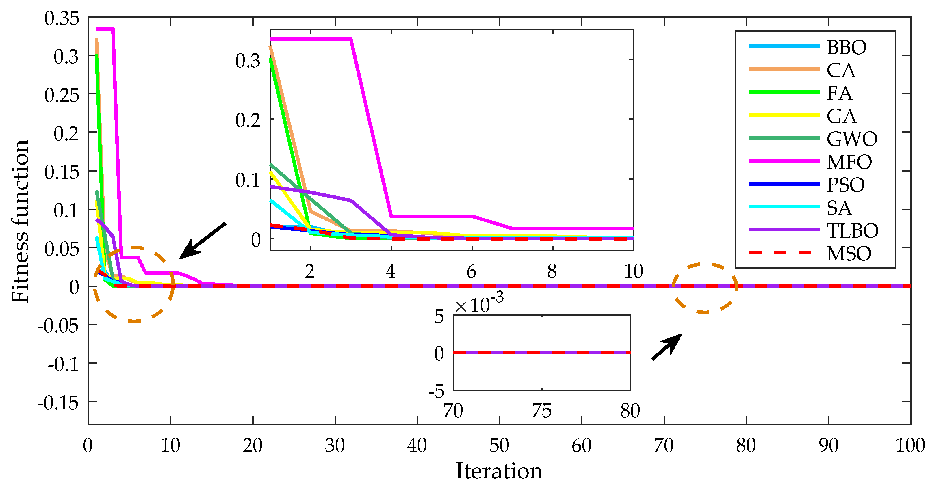
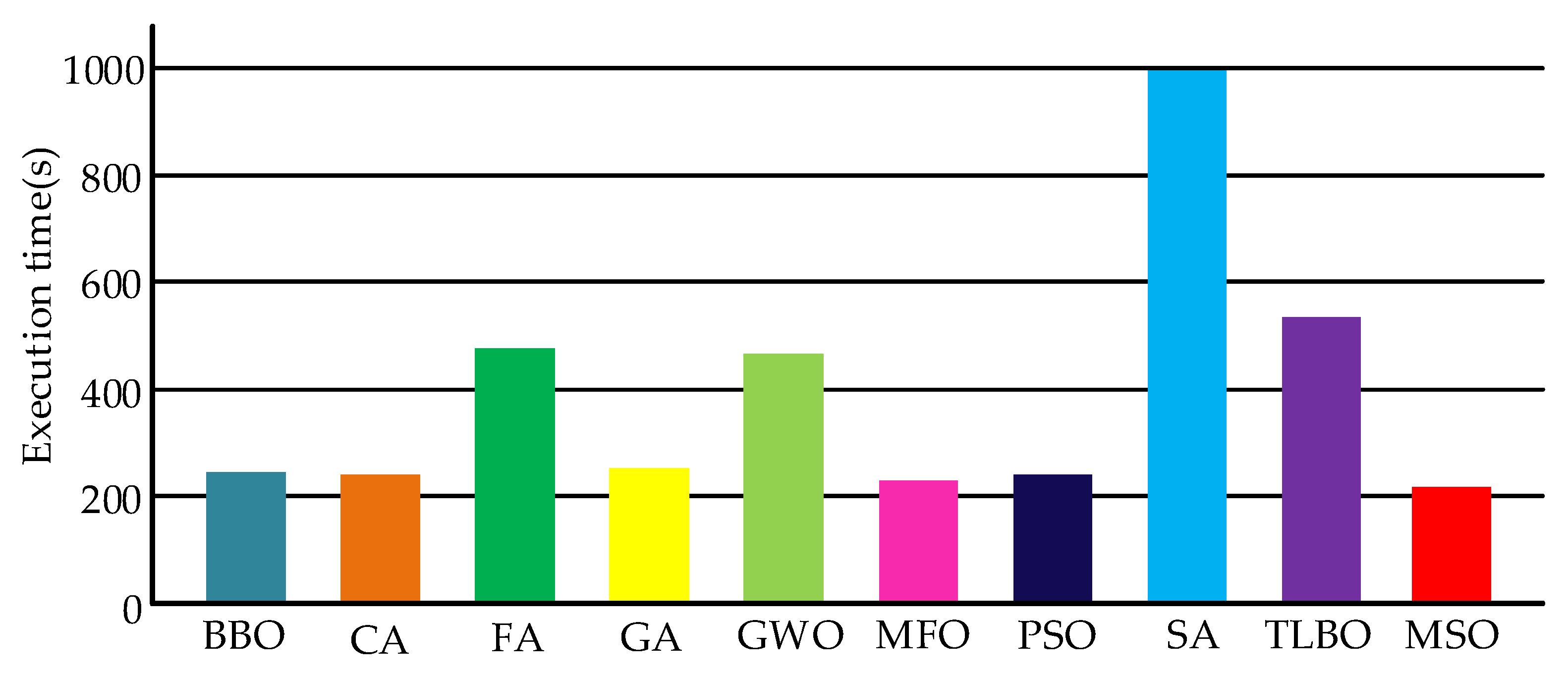
  • Through combination with the chaos theory, the global search ability of the MSO can be effectively enhanced. Besides, a double-layer searcher is designed to accelerate the convergence of MSO, while a high-quality optimal solution can be guaranteed. Compared with nine existing heuristic algorithms, the proposed MSO can search a higher quality dispatch scheme for OED within a shorter computation time.
The rest of the paper is structured as follows: Section 2 details the mathematical model of OED of combined heat and power-thermal-wind-photovoltaic systems. Section 3 gives the detailed operations of the MSO and its application for OED. A discussion and analyses of case studies is given in Section 4. Section 5 concludes the main contributions of this study.

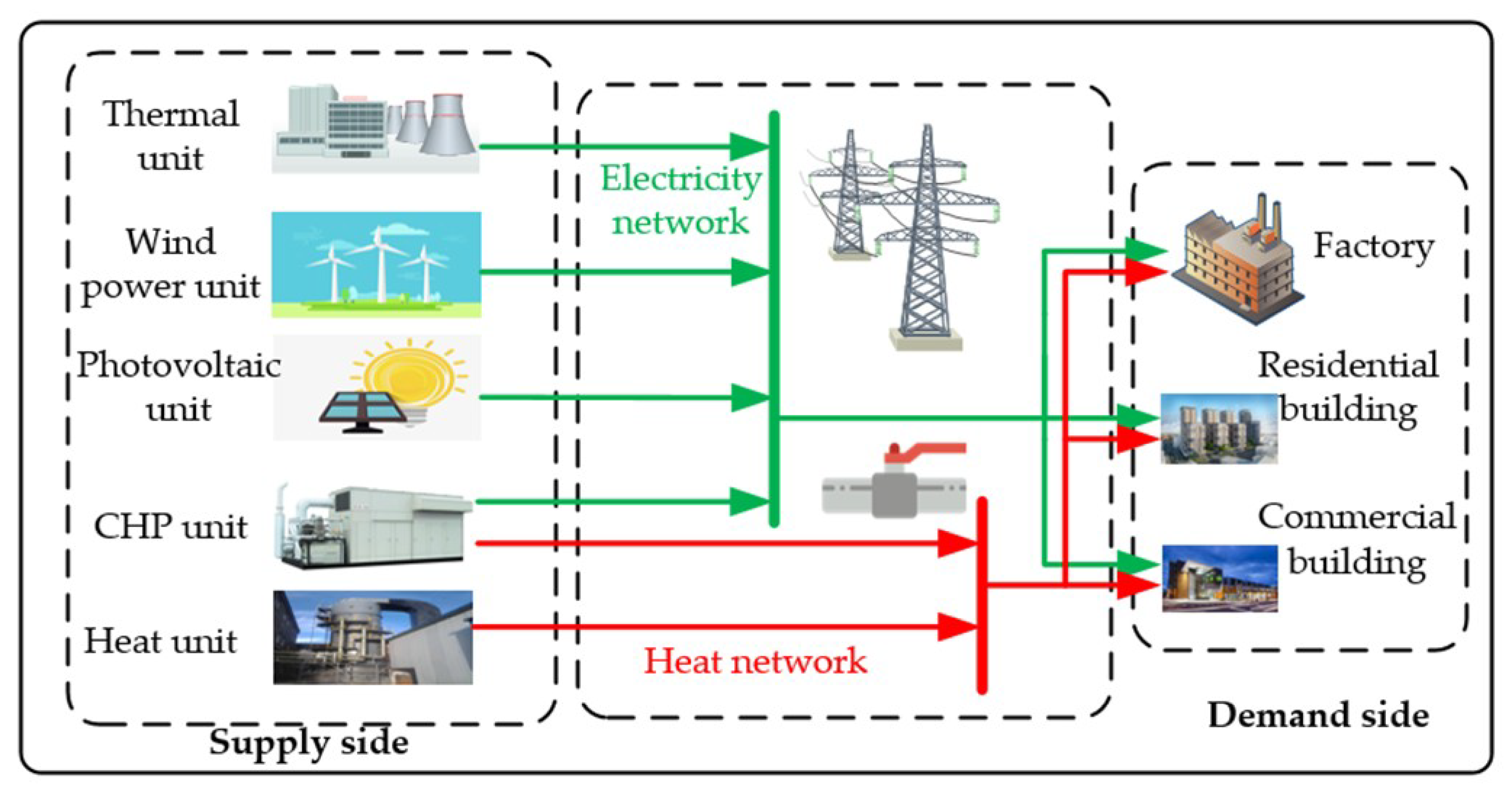
2. Mathematical Model of OED of Combined Heat and Power-Thermal-Wind-Photovoltaic Systems

The OED framework of combined heat and power-thermal-wind-photovoltaic systems is illustrated in Figure 1. The supply side consists of thermal units, combined heat and power (CHP) plants, heating plants, WT units and PV units. The generated electricity and heat energy are transmitted to the demand side through lines and pipelines. This study aims to minimize the total operating cost of the whole system while satisfying all the constraints, including energy balance constraints, the capacity limits of all energy sources and feasible operating region constraints of CHP units.

2.1. Renewable Energy

2.1.1. Relationship between Wind Speed and Wind Power Output

The power output of a WT unit is mainly determined by the probability distribution parameter of wind speed. In general, the wind speed probability distribution can be described by different models, including Weibull distribution, Rayleigh distribution, log-normal distribution, and normal distribution. Since the two-parameter Weibull model can adjust the parameters to adapt to the periodic variation of wind speed, it is the most frequently used model for wind speed probability distribution, in which the cumulative distribution function can be written as follows [15,16]:
f V ( v ) = k c ( v c ) ( k 1 ) exp [ ( v c ) k ]
F V ( v ) = 0 v f V ( ξ ) d ξ = 1 exp [ ( v c ) k ]
where V represents the speed random variable, v is the wind speed, k is the shape factor of the wind speed probability distribution function, which determines the overall shape of the wind speed probability distribution density curve, and c is the scale factor of the wind speed probability distribution function, which reflects the average wind speed of the wind field and can enlarge or reduce the curve, but does not affect the shape of the distribution density curve.
Assuming that the output characteristic of a WT is a simplified piecewise linear function, its power output can be calculated according to the given wind speed [17]:
p w t = { 0 v < v i n , v > v o u t p w t r v v i n v r v i n v i n v v r p w t r v r < v v o u t
where pwt is the current maximum power points of the WT unit, p w t r is the rated power of the WT unit, vr is the rated wind speed, v is the current wind speed, and vin and vout are the cut-in and cut-out wind speeds, respectively.
The probability distribution of wind speed is converted into the probability distribution of wind power by a linear transformation [18]:
P W T = T ( V ) = e V + f
f P W T ( p w t ) = f V [ T 1 ( p w t ) ] [ d T 1 ( p w t ) d p w t ] = f V ( p w t f e ) | 1 e |
where V and PWT are the wind speed random variable and the wind power random variable, respectively, and T represents a transformation.
For the Weibull function, the discrete part of the wind power output can be written as follows:
F P W T ( p w t = 0 ) = F V ( v i n ) + ( 1 F V ( v o u t ) ) = 1 exp ( ( v i n c ) k ) + exp ( ( v o u t c ) k )
F P W T ( p w t = p w t r ) = F V ( v o u t ) F V ( v r ) = exp ( ( v r c ) k ) exp ( ( v o u t c ) k )
If the output power of the fan is in a continuously changing range, the probability density function of the Weibull model can be described as follows:
f P W T ( p w t ) = ( k φ v i n c p w t r ) [ ( 1 + φ p w t / p w t r ) v i n c ] exp { [ ( 1 + φ p w t / p w t r ) v i n c ] k }
φ = v r v i n v i n

2.1.2. Relationship between Solar Irradiance and Solar Power Output

According to the statistics, solar irradiance is subject to Beta distribution over a certain period of time [19], whose probability density function can be written as follows:
f R ( r ) = Γ ( + ƛ ) Γ ( ) Γ ( ƛ ) ( r r max ) 1 ( 1 r r max ) ƛ 1
= μ [ μ ( 1 μ ) σ 2 1 ]
ƛ = ( 1 μ ) [ μ ( 1 μ ) σ 2 1 ]
where rmax is maximum solar irradiance, r is the solar irradiance, μ is the mean, and σ is the standard deviation.
Generally speaking, the output power of a PV cell is linearly matched with the solar irradiance. If power loss is not considered, and the influence of the ambient temperature is ignored, the output power of a PV unit can be described by [20,21]:
p p v = r A η
where A is the total area of the PV cell and η is the PV cell efficiency.
Therefore, the probability density function of the PV cell can be derived as follows:
f P P V ( p p v ) = 1 A η Γ ( + ƛ ) Γ ( ) Γ ( ƛ ) ( p p v p p v max ) 1 ( 1 p p v p p v max ) ƛ 1
where ppv is the output power of a PV cell and p p v max is the maximum generated power.

2.2. Objective Function

In this study, the objective function of OED is the minimization of the total operating cost, which can be calculated as follows:
C t o t a l = C i ( P i p ) + C j [ P j c , H j c ] + C k ( H k h ) + C w t , l ( P l ) + C p v , m ( P m )     i = 1 ,   2 , ,   N P ;    j = 1 ,   2 , ,   N c k = 1 ,   2 , ,   N k ;     l = 1 ,   2 , ,   N l ;     m = 1 ,   2 , ,   N m
where Ci ( P i p ) with i = 1, 2, …, Np represents the cost function of the ith thermal unit, Cj [ P j c , H j c ] with j = 1, 2,…, Nc represents the cost function of the jth CHP, Ck ( H k h ) with k = 1, 2,…, Nk represents the cost function of the kth heat-only unit, Cwt,l (Pl) with l = 1, 2,…, Nl represents the cost function of the lth WT unit, Cpv,m (Pm) with m = 1, 2,…, Nm represents the cost function of the mth PV unit, and Np, Nc, Nk, Nl and Nm are the number of conventional units, CHP units, heat-only units, WT units and PV units, respectively.

2.2.1. Thermal Units
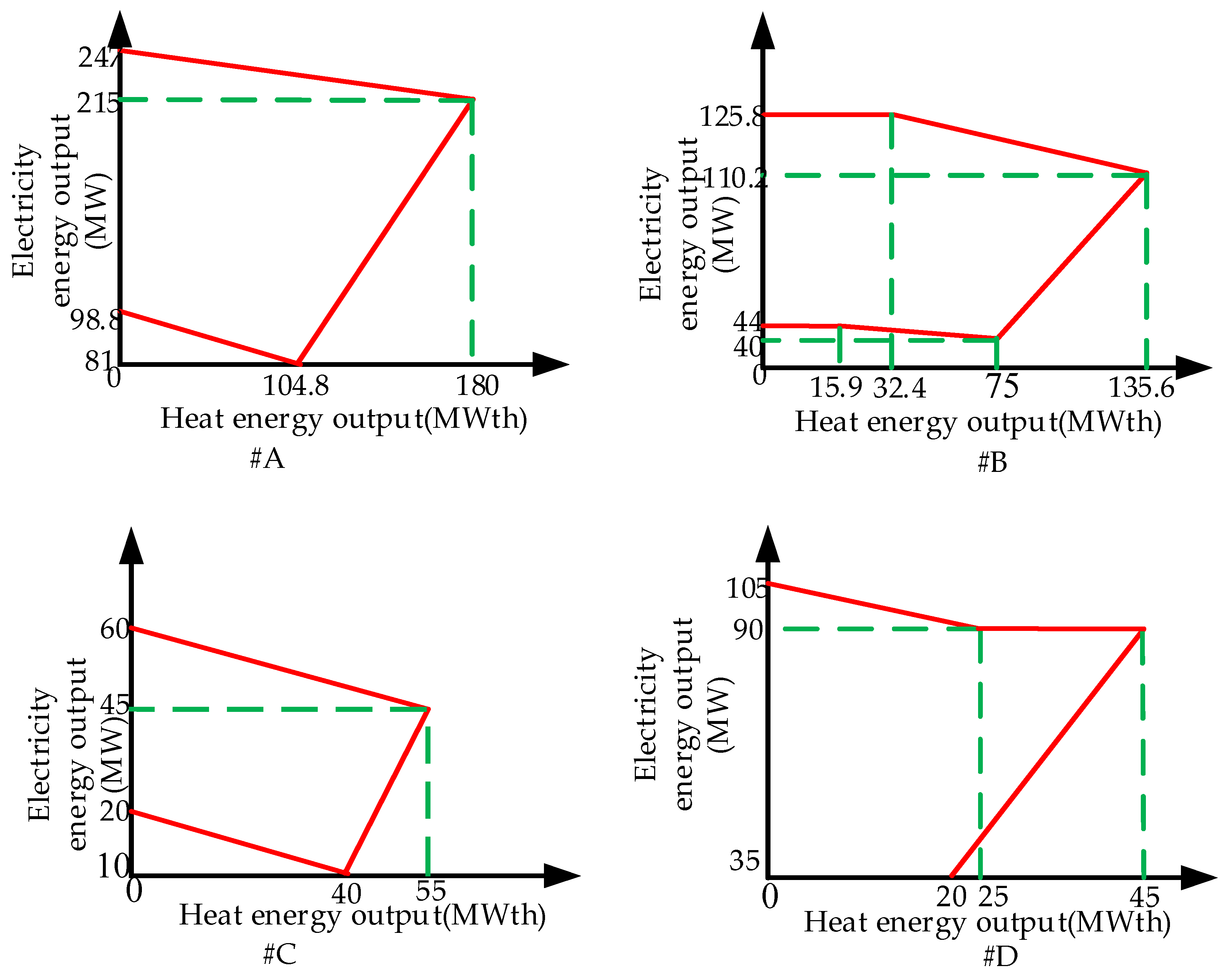
In general, the fuel cost of a thermal unit can be expressed by a quadratic function. However, a thermal unit usually has multiple valves for controlling the power output. When the steam admission valves in thermal units are first opened, a sudden increase in losses is observed. This leads to ripples in the cost function, which is known as valve-point loading. Hence, the fuel cost function needs to increase a rectified sinusoidal component by considering this effect. The operating cost of the thermal units can be written as follows [22]:
C i ( P i p ) = a i ( P i p ) 2 + b i P i p + c i + | d i sin ( e i ( P i P min P i p ) ) |      i = 1 , 2 , , N P
where ai, bi, ci, di, and fi are cost coefficients of the ith thermal unit, p i p min represents the minimum power generation limit of the ith thermal unit, and P i p is the electricity energy output of the ith thermal unit.

2.2.2. CHP Units

The CHP cost function is usually expressed as a quadratic polynomial function of the heat and electricity power output of a CHP unit, which appends a coupling coefficient that relates electricity power and heat. Hence, the operating cost of a CHP unit is determined simultaneously by its heat and electricity energy outputs, as follows [23]:
C j [ P j c , H j c ] = a j ( P j c ) 2 + b j P j c + c j + d j ( H j c ) 2 + e j H j c +   f j H j c P j c j = 1 , 2 , , N c
where aj, bj, cj, dj, ej and fj are the operating cost coefficients of the jth CHP unit, P j c is the electricity energy output of the jth CHP unit, and H j c is the heat energy output of the jth CHP unit.

2.2.3. Heat-Only Units

Compared with the CHP unit, the heat-only unit can only generate the heat energy. From the result of experiments for the generation of characteristic of heat only units, the operating cost can be described as a quadratic function [24]:
C k ( H k h ) = a k ( H k h ) 2 + b k H k h + c k k = 1 , 2 , , N k
where ak, bk and ck are the operating cost coefficients of the kth heat-only unit, and H k h is the heat energy output of the kth heat-only unit.

2.2.4. WT Units

In general, WT units are privately owned and grid operators need to purchase electricity energy from them with a power purchase agreement and a certain payment. The payment consists of three parts, in which the first part is the direct cost of buying wind power. A linear cost function can be assumed for the direct cost of WT, as follows [25]:
C d , w t , l ( P l ) = d w t , l P w t , l     l = 1 , 2 , , N l
where dwt,l is the direct cost coefficients of the lth wind power and Pwt,l is the electricity energy output of the lth wind power.
The second part is the penalty cost for underestimation of wind power output due to its high randomness. When the planned wind power is lower than the available wind power, the excess wind energy is wasted and needs to be translated into the penalty cost. The penalty cost for not using all the available wind power will be linearly related to the difference between the available wind power and the planned wind power, as follows [25]:
C u e , w t , l ( P l ) = K u e , w t , l P w t , l P w t , r a t e , l ( p w t P w t , l ) f P W T ( p w t ) d p w t     l = 1 , 2 , , N l
where Kue,wt,l is the underestimated coefficient of the lth wind power, Pwt,rate,l is the rated power generation of the lth wind power, and Pwt,l is the scheduled power generation of the lth wind power.
The third part is the ancillary cost generated by overestimated wind power output. If the scheduled wind power output is higher than the actual available wind power, then the backup power source should be obtained elsewhere to meet the load demand. Similar to the second part, the ancillary cost is also linearly related to the difference between the available wind power and the scheduled wind power, multiplied by the wind power output probability function. Hence, the ancillary cost can be calculated as:
C o e , w t , l ( P l ) = K o e , w t , l 0 P w t , l ( P w t , l p w t ) f P W T ( p w t ) d p w t     l = 1 , 2 , , N l
where Koe,wt,l is the overestimated coefficient of the lth wind power.
According to the Equations (19)–(21), the total operating cost of a wind plant can be calculated as follows:
C w t , l ( P l ) = C d , w t , l ( P l ) + C o e , w t , l ( P l ) + C u e , w t , l ( P l )     l = 1 , 2 , , N l

2.2.5. PV Units

To avoid unnecessary complexity, we assumed the cost function of PV units was similar to WT units. This addition was composed of three parts and calculated as a proposed approach [25]:
C p v , m ( P m ) = C d , p v , m ( P m ) + C o e , p v , m ( P m ) + C u e , p v , m ( P m )     m = 1 , 2 , , N m
C d , p v , m ( P m ) = d p v , m P p v , m     m = 1 , 2 , , N m
C u e , p v , m ( P m ) = K u e , p v , m P p v , m P p v , r a t e , m ( p p v P p v , m ) f P P V ( p w t ) d p w t     m = 1 , 2 , , N m
C o e , p v , m ( P m ) = K o e , p v , m 0 P p v , m ( P p v , m p p v ) f P P V ( p w t ) d p w t     m = 1 , 2 , , N m
where dpv,m is the direct cost coefficients of the mth PV power unit, Kue,pv,m is the underestimated coefficient of the mth PV unit, and Koe,pv,m is the overestimated coefficient of the mth PV unit.

2.3. Constraints

2.3.1. Equality Constraints

The energy balance constraints are the most essential requirements for OED, i.e., the electricity and heat energy outputs from the energy suppliers need to be equal to the energy demands, which can be written as follows:
i = 1 N P P i p + j = 1 N c P j c + l = 1 N l P l + m = 1 N m P m = P l o s s + P d
j = 1 N c H j c + k = 1 N k H k h = H d
where Pd and Hd represent the total electricity and heat energy demands, respectively.

2.3.2. Inequality Constraints

In order to guarantee a feasible operation, the energy output of each unit should be limited within its lower and upper bounds:
P i , min p P i p P i , max p     i = 1 , 2 , , N P
0 P w t , l P w t , r a t e     l = 1 , 2 , , N l
0 P p v , m P p v , r a t e     m = 1 , 2 , , N m
H k , min h H k h H k , max h     k = 1 , 2 , , N k
P j , min c ( H j c ) P j c ( H j c ) P j , max c ( H j c )     j = 1 , 2 , , N c
H j , min c ( P j c ) H j c ( P j c ) H j , max c ( P j c )      j = 1 , 2 , , N c
where P i , min p and P i , max p are the lower and upper bounds of the ith thermal unit, respectively, H k , min h and H k , max h are the lower and upper bounds of the kth heat-only unit, respectively, P j , min c ( H j c ) and P j , max c ( H j c ) are the lower and upper bounds of the jth CHP unit, respectively, and H j , min c ( P j c ) and H j , max c ( P j c ) are the lower and upper bounds of the jth CHP unit, respectively.
It can be found from Equations (33) and (34) that the heat energy output of the CHP unit will directly influence its lower and upper bounds of the electricity energy output and vice versa. This coupling relationship is usually described by a feasible operating region constraint, i.e., the energy outputs of the CHP unit must be enclosed by the boundary curve ABCDEF, as illustrated in Figure 2. The BC along the boundary line of the area increases the heat energy output of the unit and the electricity energy output decreases. The heat energy output by the CD unit along the line is decremented.

3. Multi-Searcher Optimization

Most of the existing metaheuristic algorithms are inspired by nature phenomena, and the proposed MSO is developed from their advantages and the chaos theory. Overall, the MSO consists of a two-layer searcher, in which the first-layer searcher is responsible for a wide global search and the second-layer searcher is implemented for a deep local search.

3.1. Chaos Theory

In many practical systems, chaos is a ubiquitous non-linear phenomenon. Chaotic motion can reach every state of a certain scale, according to its regularity and ergodicity, which is better than a simple random search. Therefore, for many optimization algorithms, chaotic theory is frequently used to introduce random parameters in the initialization solution or the replacement algorithm to enhance ergodicity and accelerate global optimal convergence [26]. Due to the non-repetitive nature of chaos, the chaotic mapping-based optimization algorithm has more comprehensive search ability than the original one. This feature can make the optimization algorithm effectively escape a low- quality local optimum and avoid the premature convergence.
Here, the logistic mapping formula is used to generate the chaotic variables with chaotic state during the initialization process, thereby, the chaotic iterative formula can be written as follows:
Z t + 1 = κ Z t ( 1 Z t ) t = 0 , 1 , 2 , κ ( 0 , 4 ]
where Zt is the tth chaotic vector and κ is a positive real parameter, i.e., the controllable variables of the optimization.
A n-dimensional chaotic vector Z0 (Z0 = z01, z02, …, z0n) is randomly generated and each component value is between 0 and 1. On the basis of the chaotic iterative formula and the n-dimensional chaotic vector Z0 (Z0 = z01, z02, …, z0n), the N vectors Z1 (Z1 = z11, z12, …, z1n), Z2 (Z2 = z21, z22, …, z2n), …, ZN (ZN = zN1, zN2, …, zNn) can be obtained by iteration. The chaotic vector is used for the iterative search and then the component of the chaotic vector Zi (i = 1, 2, …, N) is transformed into the constraint range of Equations (29)–(32) by Equation (36), as follows:
x i j = x min + z i j × ( x max x min )    i = 1 , 2 , , N ; j = 1 , 2 , , n
where xmin and xmax are the lower and upper limits of the optimization variable, respectively.

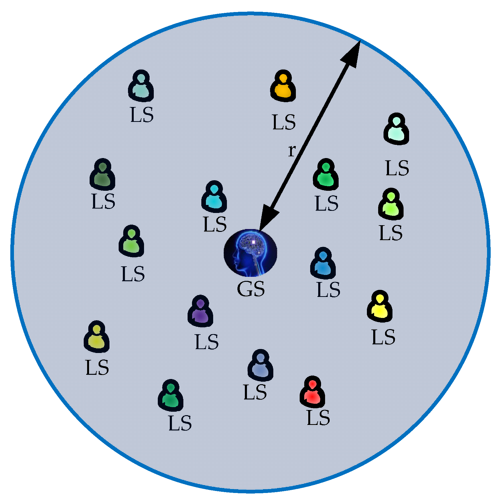
3.2. Double Layer Searcher

As shown in Figure 3, in the process of initialization, a series of searchers are randomly distributed within the search area by using Equation (36), which is the so-called global searcher (GS) in the MSO. Surrounded by each global searcher and centered around this searcher within a specified radius, some other searchers are randomly distributed, known as local searchers (LS), which are subject to the global searcher. These LS aims to perceive the surrounding dynamic change process in the vicinity of each GS and then perform a local search. When the searching process of the GS is finished, the LS will initiate a subsequent search. This feature can effectively improve the convergence speed and avoid a low-quality local optimum.
The search radius of the GS depends on the distance from the global best (Gbest) and the level of each global searcher. The level will be equal to 0 if a global searcher is finding the minimum cost, and vice versa. Hence, the search radius of the GS is calculated as follows:
r = max { ( r max r min ) k G S n G S 1 + r min , d i s t ( GS , Gbest ) }
where rmax and rmin are the pre-set maximum and minimum radii, kGS represents the level of GS, nGS is the number of global searchers, Gbest is described as the global optimal solution, and dist (GS,Gbest) denotes the distance between the global searcher and the global best.

3.3. Random Walk Rule

To randomly move from one position to another, the searcher should consider two variables, including the distance and direction angle. The distance is determined by a coefficient of the distance between two points, and the direction angle is a random value. The distance between the global searcher and the global best (known as d) is found by using Equation (37). λ is a random value with a distribution of uniform probability in a range from 0 to 1, and Ɵ is a random value with a distribution of uniform probability in a range from -π/4 to π/4. When all global searchers move according to the random walk rule, the new position can be obtained, and the obtained solution will be compared with the current global optimal solution. If the solution quality is higher, the global optimal solution will be replaced.
As shown in Figure 4, after searching using the LS, each GS begins to move to a new position by a random motion technique called ‘‘random walk’’. Movement in the random walk is done from a point toward the target position, which leads to the GS being located in the area around the target position.

3.4. Constraint Processing

In this paper, all equality constraints (Equations (27)–(28)) are processed by the penalty function method to avoid the “over limit” phenomenon. The equality constraint optimization is transformed into a problem without an equality constraint, and the fitness function is constructed by using a penalty coefficient M, which is as follows:
C t o t a l = C i ( P i p ) + C j [ P j c , H j c ] + C k ( H k h ) + C w t , l ( P l ) + C p v , m ( P m )   + M | P i p + P j c + P l + P m P l o s s P d | + M | H j c + H k h H d |
Moreover, the penalty factor M is used for guaranteeing a feasible solution for the proposed OED. In general, a larger M can effectively avoid an infeasible solution, but easily results in a low optimization accuracy. Hence, the penalty factor M should be carefully set via a proper balance between the constraint violation and the optimization accuracy. Through trial-and-error, it was set to be 107 for OED. Obviously, when the equality constraint is satisfied, the penalty function is equal to 0, and the value of the fitness function is the cost function.

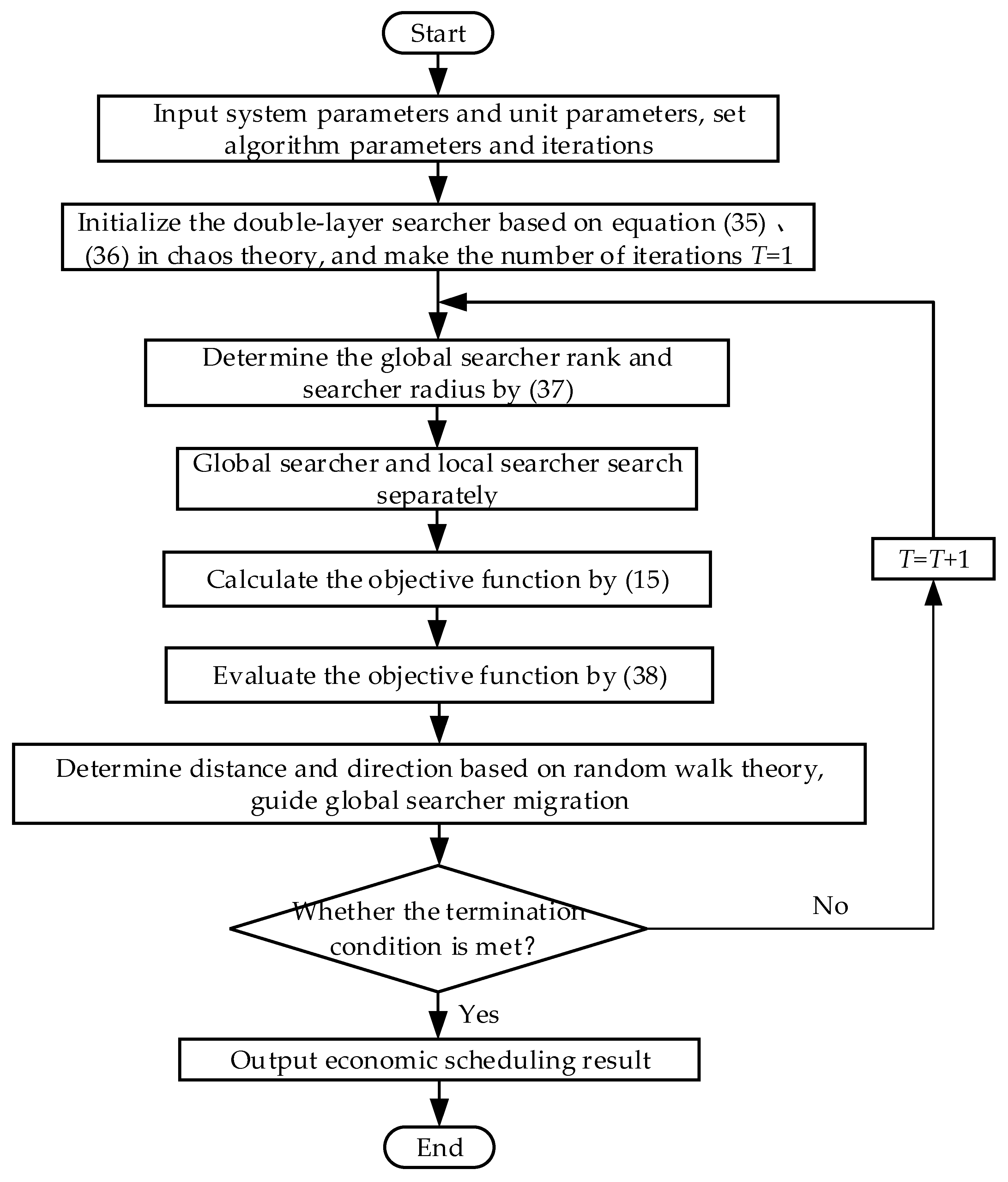
3.5. Execution Procedure

In order to solve a specific optimization problem, the number of optimization variables, constraints, and the objective function should be given to the proposed MSO. In fact, the number of optimization variables will determine the parameters setting of the MSO, while the fitness function is completely dependent on both of the objective function and constraints. Therefore, the proposed MSO can be used for addressing different benchmark test functions or the proposed OED.
At last, the overall execution procedure of the MSO for OED is given in the Figure 5.
  • Step 1: Input system parameters and unit parameters, including the operating cost coefficients of the thermal units, CHP units and heat-only units, the feasible operating region of the CHP units, and the main parameters of renewable energy resources such as wind speed and solar irradiance. Set the algorithm parameters, including the number of GS, the number of LS, the maximum search radius, minimum search radius, and the maximum iteration number.
  • Step 2: Initialize the double-layer searcher based on Equations (35)–(36) in chaos theory; and set the current iteration number T = 1.
  • Step 3: Determine the global searcher level and searcher radius with Equation (37). Particularly, the level 0 is assigned to the GS corresponding to the least cost, and the highest level is assigned to the GS corresponding to the highest cost.
  • Step 4: Implement the global searcher and local searcher separately, where the local searcher is surrounded by each global searcher and centered around the searcher within a specified radius.
  • Step 5: Calculate the objective function with Equation (15), which is equal to the total operating cost.
  • Step 6: Evaluate the objective function using the penalty function method from Equation (38), based on the given M.
  • Step 7: Determine the distance and direction based on random walk theory and guide global searcher migration, in which both λ and Ɵ are the random values with a distribution of uniform probability.
  • Step 8: Judge the termination of MSO. If the termination condition is met, then output the economic scheduling result, else turn to step 3 and enter the next iteration.

4. Case Studies

In order to test the optimization effect of the MSO for the OED of combined heat and power-thermal-wind-photovoltaic systems, this paper introduces nine commonly used heuristic algorithms which are highly independent from a specific mathematical model, including biogeography-based optimization (BBO) [27], cultural algorithms (CA) [28], firefly algorithms (FA) [29], genetic algorithms (GA) [11], the grey wolf optimizer (GWO) [14], moth-flame optimization (MFO) [30], particle swarm optimization (PSO) [12], simulated annealing (SA) [31] and a teach-learn based optimization algorithm (TLBO) [32].
Through trial-and-error, the main parameters of different algorithms are given in Table 1. All the simulations were undertaken in MATLAB R2016b on a personal computer with an Intel(R) Core TM i7 CPU at 3.4 GHz with 16 GB of RAM.
In order to assure a fair comparison, all the parameters of each algorithm have been carefully set based on two rules, as follows:
(1) Common parameters: The maximum iteration number and the population size are the common parameters of all of the algorithms, which should be set to the same values for each algorithm. Generally speaking, both a larger maximum iteration number and a larger population size can effectively obtain a higher quality optimum, however, this consumes more computation time. Hence, these two parameters were set to achieve a proper balance between the optimum quality and the computation time. Through trial-and-error, they were set to be 300 and 150 for all the algorithms, respectively.
(2) Independent parameters: Each algorithm has its own parameters, e.g., the crossover probability of GA and the maximum velocity of PSO. These parameters can be determined according to the optimum quality with the given maximum iteration number and population size. Through trial-and-error, the optimal parameters are given in Table 1.

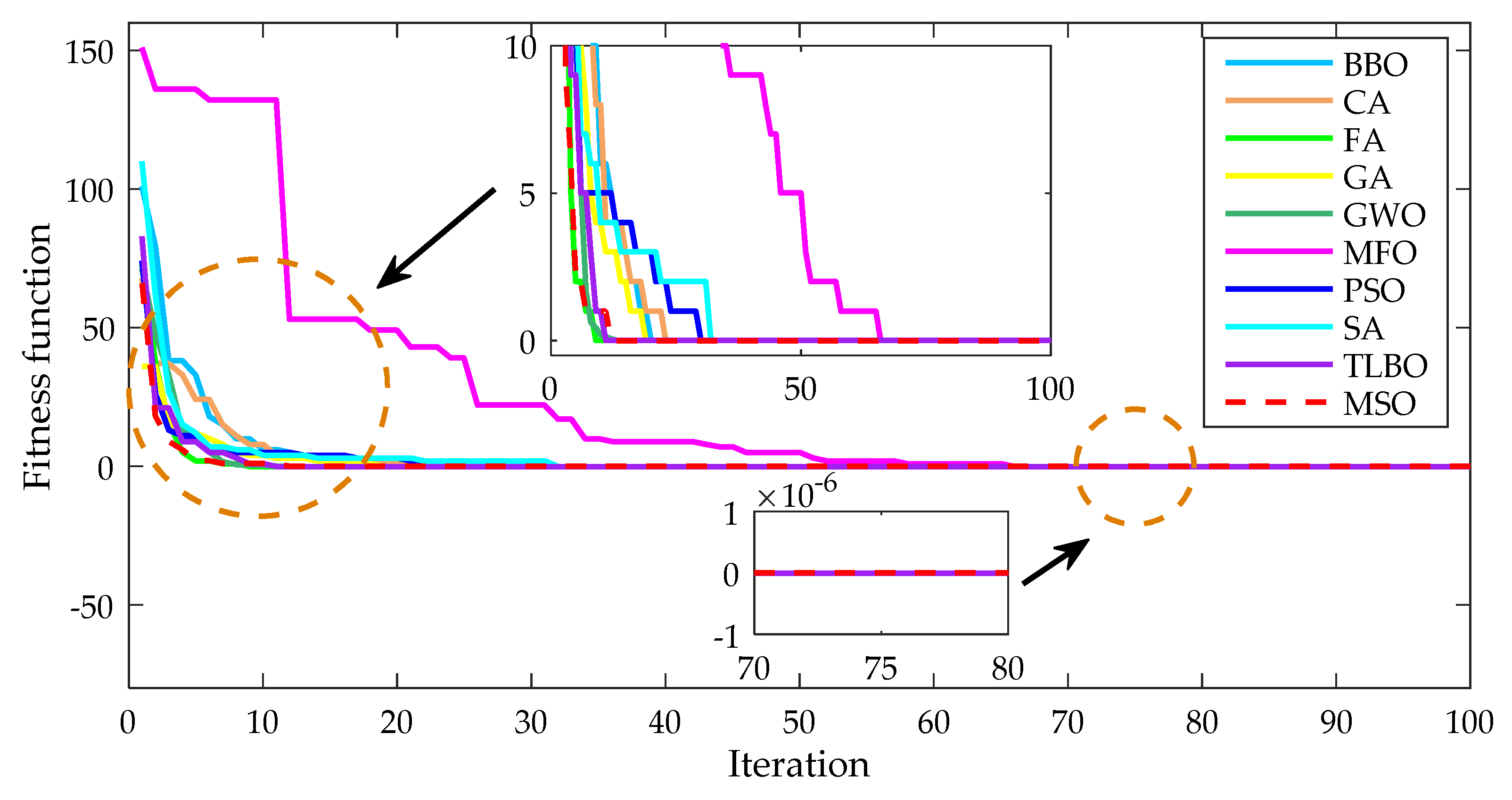
4.1. Benchmark Test Function

In order to verify the validity of the algorithm, three different types of functions were selected for numerical experiments. The number of iteration steps was set to 100.
The Sphere function is a simpler unimodal function that examines the convergence speed of the algorithm, where the mathematical model can be written as follows:
min f ( x ) = i = 1 n x i 2 , n = 2 , | x i | 5.12
The global advantage is xi = 0, f(x) = 0. The comparison of the fitness convergence curves in the unimodal function is shown in the Figure 6. It can be seen that the MSO can converge to the global optimum with a fastest convergence rate compared to the other nine algorithms.
The step function is a discontinuous step function that can be used to verify the validity of the algorithm, which can be described as follows:
min f ( x ) = i = 1 n ( x i + 0 , 5 ) 2 , n = 5 , | x i | 10
The global best advantage is xi = 0, f(x) = 0. The comparison results of the fitness convergence curves of the discontinuous step function are shown in the Figure 7. Similarly, the proposed MSO also had the fastest convergence rate among all of the algorithms, while a global optimum could be guaranteed.
The Rastrigin function is a multimodal function that can be used to test the algorithm’s ability to jump out of local optimum, which can be described as follows:
min f ( x ) = 10 n + i = 1 n x i 2 10 cos ( 2 π x i ) , n = 2 , | x i | 5.12
The global best advantage is xi = 0, f(x) = 0. The comparison results of the fitness convergence curves of the discontinuous step function are shown in the Figure 8. It can be seen that the global optimization ability of the MSO was more obvious, and other comparison algorithms were trapped in a low-quality local optimum.
In the figures (like Figure 6), the MSO seems to have an advantage immediately in iteration 0 or 1. The main reason for this is that the MSO adopts chaotic mapping for the population initialization, which can reach every state of a certain scale due to its regularity and ergodicity. On the other hand, the other algorithms only adopt a simple random search-based initialization, such that they easily lead to a low optimization efficiency during the initialization process. Hence, the MSO can effectively obtain a higher quality initial best solution compared to other algorithms.

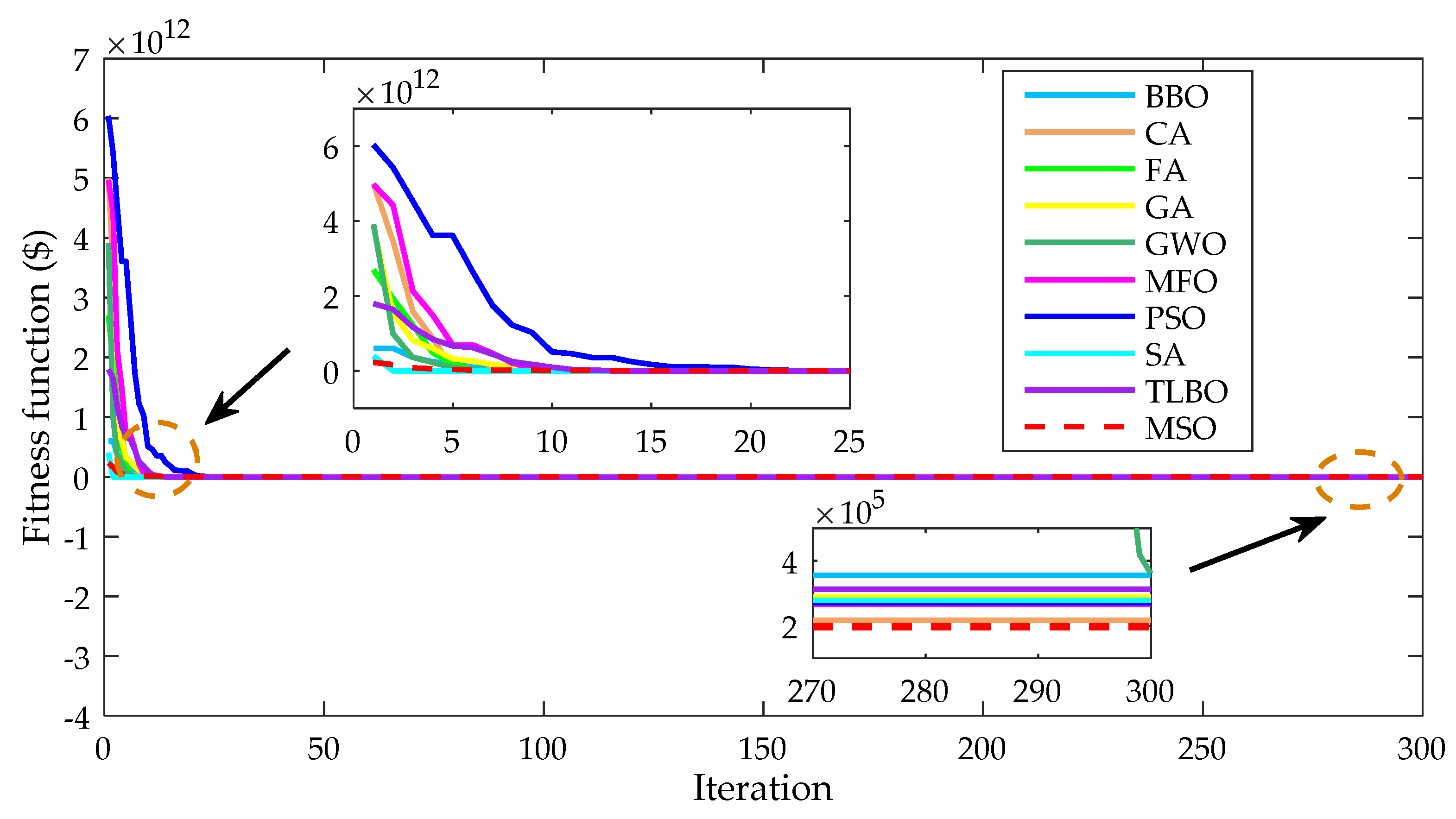
4.2. Simulation Model

The test system included 13 thermal units with the valve point effect, 4 CHP units, 4 heat-only units, 3 WT units and 3 PV units. The proposed OED was implemented as a day-ahead or hour-ahead dispatch, thereby the demand profile was determined by the day-ahead or hour-ahead load forecasting according to the historical demand data [33,34,35]. The total electricity energy demand was 3837.136MW and total heat energy demand was 615.372MWth.
The main parameters of the thermal units, CHP units and heat-only units are provided in Table 2, Table 3 and Table 4, respectively. The feasible operating region of the CHP unit is shown in Figure 9. The main parameters of renewable energy resources are given in Table 5. All the parameters of the energy sources are steady values, which are usually acquired from the energy suppliers when they connect into the integrated energy system. In this paper, these parameters were referred from the published papers [18,36,37,38,39,40]. The capacities of the WT units in these papers were 130 MW, 94 MW and 94 MW, respectively. Moreover, the capacity of the PV unit was 150 MW, separately. The maximum iteration number of each algorithm was set to 300.

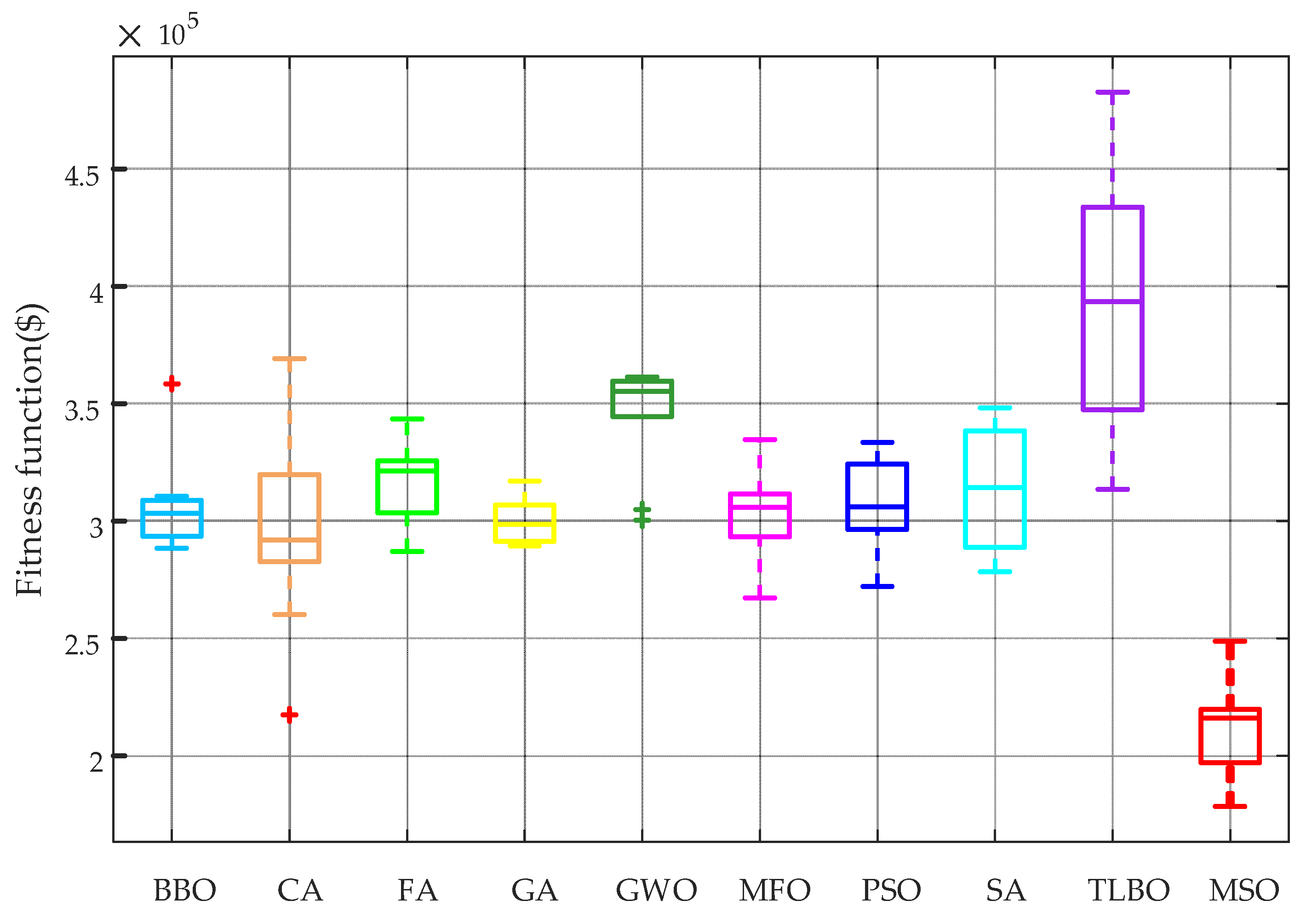
4.3. Discussion and Analysis

Figure 10 shows the convergence of total operating costs obtained by different algorithms and the detailed optimal dispatch strategies of all the energy suppliers obtained by different algorithms are listed in Table 6. It can be seen that the MSO obtains the lowest total operating cost, which can verify that the MSO can effectively jump out of a low-quality local optimum. The MSO started to converge after 114 iterations.
Figure 11 represents the box and whisker plots of various algorithms that were ran ten times. From the comparison of the box and whisker diagrams, it can be found that the convergence stability of the MSO was not as good as GA and GWO, but the range of variation was still acceptable, and the fitness function was lower than that of GA and GWO.
In order to verify the calculation speed of the MSO, Figure 12 shows the average execution time comparison bar graph, obtained by running the various algorithms 10 times. It was found that the execution time of MSO was the shortest among all the algorithms, which was about 4.96 times faster than SA.

5. Conclusions

In this paper, a novel MSO is proposed for the OED of combined heat and power-thermal-wind- photovoltaic systems, which has the following advantages:
  • The introduction of chaos theory can effectively maintain the non-repetition of the initial population and the diversity of the searcher, which can improve the global search ability of MSO.
  • The double-layer searcher can effectively make the proposed MSO quickly converge to the best advantage, and avoid the defects that cause the traditional heuristic algorithm to easily fall into a low-quality local optimum.
  • The superior performance of the MSO was verified by the benchmark test function and a specific engineering optimization of OED, compared with various heuristic algorithms.
The next research work will integrate the migration learning into the MSO reasonably, and consider the actual loss of the network, and apply it to a more complex optimization.

Author Contributions

Methodology, X.Z.; Investigation, J.C.; Data curation, Z.L.; Formal analysis, J.T.; Writing—original draft preparation, J.T.; Writing—review and editing, X.Z.; Supervision, T.Y.

Funding

This research was funded by the National Natural Science Foundation of China (Grant. 51477055&51777078).

Acknowledgments

The authors gratefully acknowledge the support of the National Natural Science Foundation of China.

Conflicts of Interest

The authors declare no conflict of interest.

Nomenclature

EDEconomic dispatch
IESIntegrated energy system
WTWind turbine
PVPhotovoltaic
OMEFOptimal multi-energy flow
MABLMulti-agent bargaining learning
EHEDEnergy hub economic dispatch
MECSMultiple energy carrier systems
OEDOptimal energy dispatch
GAGenetic algorithm
PSOParticle swarm optimization
DEDifferential evolution
GWOGrey wolf optimizer
MSOMulti-searcher optimization
CHPCombined heat and power
GSGlobal searcher
LSLocal searcher
BBOBiogeography-based optimization
CACultural algorithm
FAFirefly algorithm
MFOMoth-flame optimization
SASimulated annealing
TLBOTeach-learn based optimization algorithm
VSpeed random variable
vWind speed
kShape factor of the wind speed probability distribution function
cScale factor of the wind speed probability distribution function
pwtCurrent maximum power points of wind turbines unit
p w t r Rated power of WT unit
vrRated wind speed
vin, voutCut-in and cut-out wind speeds, respectively
PWTWind power random variable
rmaxMaximum solar irradiance
rSolar irradiance
ATotal area of the photovoltaic cell
ppvOutput power of a PV cell
p p v max Maximum generated power
Ci ( P i p )Cost function of the ith thermal unit
Cj [ P j c , H j c ]Cost function of the jth CHP
Ck ( H k h )Cost function of the kth heat-only unit
Cwt,l (Pl)Cost function of the lth WT unit
Cpv,m (Pm)Cost function of the mth PV unit
p i p min Minimum power generation limit of the ith thermal unit
P i p Electricity energy output of the ith thermal unit
P j c Electricity energy output of the jth CHP unit
H j c Heat energy output of the jth CHP unit
H k h Heat energy output of the kth heat-only unit
dwt,lDirect cost coefficients of the lth wind power
Pwt,lElectricity energy output of the lth wind power
Kue,wt,lUnderestimated coefficient of the lth wind power
Pwt,rate,lRated power generation of the lth wind power
Pwt,lScheduled power generation of the lth wind power
Koe,wt,lOverestimated coefficient of the lth wind power
dpv,mDirect cost coefficients of the mth PV power unit
Kue,pv,mUnderestimated coefficient of the mth PV unit
Koe,pv,mOverestimated coefficient of the mth PV unit
Pd, HdTotal electricity and heat energy demands, respectively
P i , min p , P i , max p Lower and upper bounds of the ith thermal unit, respectively
H k , min h , H k , max h Lower and upper bounds of the kth heat-only unit, respectively
P j , min c ( H j c ), P j , max c ( H j c )Lower and upper bounds of the jth CHP unit, respectively
H j , min c ( P j c ), H j , max c ( P j c )Lower and upper bounds of the jth CHP unit, respectively
xmin, xmaxLower and upper limits of the optimization variable, respectively
rmax, rminPre-set maximum and minimum radius
kGSLevel of GS
nGSNumber of global searchers
GbestGlobal optimal solution
dist(GS,Gbest)Distance between the global searcher and the global best
ƟDirection angle
λRandom value with a distribution of uniform probability in the range of 0–1

References

  1. Li, Y.-S.; Zhang, H.-G.; Huang, B.-N.; Teng, F. Distributed Optimal Economic Dispatch Based on Multi-Agent System Framework in Combined Heat and Power Systems. Appl. Sci. 2016, 6, 308. [Google Scholar] [CrossRef]
  2. Shao, C.; Ding, Y.; Wang, J.; Song, Y. Modeling and Integration of Flexible Demand in Heat and Electricity Integrated Energy System. IEEE Trans. Sustain. Energy 2018, 9, 361–370. [Google Scholar] [CrossRef]
  3. Li, J.; Niu, D.; Wu, M.; Wang, Y.; Li, F.; Dong, H. Research on Battery Energy Storage as Backup Power in the Operation Optimization of a Regional Integrated Energy System. Energies 2018, 11, 2990. [Google Scholar] [CrossRef]
  4. Qu, K.; Yu, T.; Huang, L.; Yang, B.; Zhang, X. Decentralized optimal multi-energy flow of large-scale integrated energy systems in a carbon trading market. Energy 2018, 149, 779–791. [Google Scholar] [CrossRef]
  5. Wang, Y.; Yu, H.; Yong, M.; Huang, Y.; Zhang, F.; Wang, X. Optimal Scheduling of Integrated Energy Systems with Combined Heat and Power Generation, Photovoltaic and Energy Storage Considering Battery Lifetime Loss. Energies 2018, 11, 1676. [Google Scholar] [CrossRef]
  6. Zhang, X.; Yu, T.; Zhang, Z.; Tang, J. Multi-Agent Bargaining Learning for Distributed Energy Hub Economic Dispatch. IEEE Access 2018, 6, 39564–39573. [Google Scholar] [CrossRef]
  7. Borowy, B.S.; Salameh, Z.M. Optimum photovoltaic array size for a hybrid wind/PV system. IEEE Trans. Energy Convers. 1994, 9, 482–488. [Google Scholar] [CrossRef]
  8. Wang, M.Q.; Gooi, H.B.; Chen, S.X.; Lu, S. A Mixed Integer Quadratic Programming for Dynamic Economic Dispatch with Valve Point Effect. IEEE Trans. Power Syst. 2014, 29, 2097–2106. [Google Scholar] [CrossRef]
  9. Lin, W.-M.; Chen, S.-J. Bid-based dynamic economic dispatch with an efficient interior point algorithm. Int. J. Electr. Power Energy Syst. 2002, 24, 51–57. [Google Scholar] [CrossRef]
  10. Ramanathan, R. Fast Economic Dispatch Based on the Penalty Factors from Newton’s Method. IEEE Trans. Power App. Syst. 1985, PAS-104, 1624–1629. [Google Scholar] [CrossRef]
  11. Bakhshi, R.; Sadeh, J.; Mosaddegh, H.-R. Optimal economic designing of grid-connected photovoltaic systems with multiple inverters using linear and nonlinear module models based on Genetic Algorithm. Renew. Energy 2014, 72, 386–394. [Google Scholar] [CrossRef]
  12. Deng, W.; Zhao, H.; Yang, X.; Xiong, J.; Sun, M.; Li, B. Study on an improved adaptive PSO algorithm for solving multi-objective gate assignment. Appl. Soft Comput. 2017, 59, 288–302. [Google Scholar] [CrossRef]
  13. Dai, S.; Niu, D.; Han, Y. Forecasting of Power Grid Investment in China Based on Support Vector Machine Optimized by Differential Evolution Algorithm and Grey Wolf Optimization Algorithm. Appl. Sci. 2018, 8, 636. [Google Scholar] [CrossRef]
  14. Yang, B.; Zhang, X.; Yu, T.; Shu, H.; Fang, Z. Grouped grey wolf optimizer for maximum power point tracking of doubly-fed induction generator based wind turbine. Energy Convers. Manag. 2017, 133, 427–443. [Google Scholar] [CrossRef]
  15. Wang, L.; Zhou, Y.; Xu, J. Optimal Irregular Wind Farm Design for Continuous Placement of Wind Turbines with a Two-Dimensional Jensen-Gaussian Wake Model. Appl. Sci. 2018, 8, 2660. [Google Scholar] [CrossRef]
  16. Carta, J.A.; Ramírez, P. Analysis of two-component mixture Weibull statistics for estimation of wind speed distributions. Renew. Energy 2007, 32, 518–531. [Google Scholar] [CrossRef]
  17. Liu, Z.; Chen, C.; Yuan, J. Hybrid energy scheduling in a renewable micro grid. Appl. Sci. 2015, 5, 516–531. [Google Scholar] [CrossRef]
  18. Hetzer, J.; Yu, D.C.; Bhattarai, K. An Economic Dispatch Model Incorporating Wind Power. IEEE Trans. Energy Convers. 2008, 23, 603–611. [Google Scholar] [CrossRef]
  19. Salameh, Z.M.; Borowy, B.S.; Amin, A.R.A. Photovoltaic module-site matching based on the capacity factors. IEEE Trans. Energy Convers. 1995, 10, 326–332. [Google Scholar] [CrossRef]
  20. Chen, S.X.; Gooi, H.B.; Wang, M.Q. Sizing of Energy Storage for Microgrids. IEEE Trans. Smart Grid 2012, 3, 142–151. [Google Scholar] [CrossRef]
  21. Yang, B.; Yu, T.; Zhang, X.; Li, H.; Shu, H.; Sang, Y.; Jiang, L. Dynamic leader based collective intelligence for maximum power point tracking of PV systems affected by partial shading condition. Energy Convers. Manag. 2019, 179, 286–303. [Google Scholar] [CrossRef]
  22. Bouchekara, H.R.E.H.; Chaib, A.E.; Abido, M.A. Optimal power flow using GA with a new multi-parent crossover considering: Prohibited zones, valve-point effect, multi-fuels and emission. Electr. Eng. 2018, 100, 151–165. [Google Scholar] [CrossRef]
  23. Dinh, B.H.; Nguyen, T.T.; Quynh, N.V.; Van Dai, L. A Novel Method for Economic Dispatch of Combined Heat and Power Generation. Energies 2018, 11, 3113. [Google Scholar] [CrossRef]
  24. Aghaei, J.; Alizadeh, M.-I. Multi-objective self-scheduling of CHP (combined heat and power)-based microgrids considering demand response programs and ESSs (energy storage systems). Energy 2013, 55, 1044–1054. [Google Scholar] [CrossRef]
  25. Morshed, M.J.; Hmida, J.B.; Fekih, A. A probabilistic multi-objective approach for power flow optimization in hybrid wind-PV-PEV systems. Appl. Energy 2018, 211, 1136–1149. [Google Scholar] [CrossRef]
  26. Liang, H.; Liu, Y.; Shen, Y.; Li, F.; Man, Y. A Hybrid Bat Algorithm for Economic Dispatch with Random Wind Power. IEEE Trans. Power Syst. 2018, 33, 5052–5061. [Google Scholar] [CrossRef]
  27. Bhattacharya, A.; Chattopadhyay, P.K. Biogeography-Based Optimization for Different Economic Load Dispatch Problems. IEEE Trans. Power Syst. 2010, 25, 1064–1077. [Google Scholar] [CrossRef]
  28. Freitas, C.A.O.D.; de Oliveira, R.C.L.; Silva, D.J.A.D.; Leite, J.C.; Junior, J.D.A.B. Solution to Economic—Emission Load Dispatch by Cultural Algorithm Combined with Local Search: Case Study. IEEE Access 2018, 6, 64023–64040. [Google Scholar] [CrossRef]
  29. Yang, X.-S.; Sadat Hosseini, S.S.; Gandomi, A.H. Firefly Algorithm for solving non-convex economic dispatch problems with valve loading effect. Appl. Soft Comput. 2012, 12, 1180–1186. [Google Scholar] [CrossRef]
  30. Li, C.; Li, S.; Liu, Y. A least squares support vector machine model optimized by moth-flame optimization algorithm for annual power load forecasting. Appl. Intell. 2016, 45, 1166–1178. [Google Scholar] [CrossRef]
  31. Xu, T.; Meng, H.; Zhu, J.; Wei, W.; Zhao, H.; Yang, H.; Li, Z.; Ren, Y. Considering the Life-Cycle Cost of Distributed Energy-Storage Planning in Distribution Grids. Appl. Sci. 2018, 8, 2615. [Google Scholar] [CrossRef]
  32. Nadeem, Z.; Javaid, N.; Malik, A.W.; Iqbal, S. Scheduling Appliances with GA, TLBO, FA, OSR and Their Hybrids Using Chance Constrained Optimization for Smart Homes. Energies 2018, 11, 888. [Google Scholar] [CrossRef]
  33. Yang, Y.; Li, S.; Li, W.; Qu, M. Power load probability density forecasting using Gaussian process quantile regression. Appl. Energy 2018, 213, 499–509. [Google Scholar] [CrossRef]
  34. Suryanarayana, G.; Lago, J.; Geysen, D.; Aleksiejuk, P.; Johansson, C. Thermal load forecasting in district heating networks using deep learning and advanced feature selection methods. Energy 2018, 157, 141–149. [Google Scholar] [CrossRef]
  35. Ahmad, T.; Chen, H. Short and medium-term forecasting of cooling and heating load demand in building environment with data-mining based approaches. Energy Build. 2018, 166, 460–476. [Google Scholar] [CrossRef]
  36. Mohammadi-Ivatloo, B.; Moradi-Dalvand, M.; Rabiee, A. Combined heat and power economic dispatch problem solution using particle swarm optimization with time varying acceleration coefficients. Electr. Power Syst. Res. 2013, 95, 9–18. [Google Scholar] [CrossRef]
  37. Beigvand, S.D.; Abdi, H.; La Scala, M. Combined heat and power economic dispatch problem using gravitational search algorithm. Electr. Power Syst. Res. 2016, 133, 160–172. [Google Scholar] [CrossRef]
  38. Piperagkas, G.S.; Anastasiadis, A.G.; Hatziargyriou, N.D. Stochastic PSO-based heat and power dispatch under environmental constraints incorporating CHP and wind power units. Electr. Power Syst. Res. 2011, 81, 209–218. [Google Scholar] [CrossRef]
  39. Zhao, J.; Wen, F.; Dong, Z.Y.; Xue, Y.; Wong, K.P. Optimal Dispatch of Electric Vehicles and Wind Power Using Enhanced Particle Swarm Optimization. IEEE Trans. Ind. Inform. 2012, 8, 889–899. [Google Scholar] [CrossRef]
  40. Karaki, S.H.; Chedid, R.B.; Ramadan, R. Probabilistic performance assessment of autonomous solar-wind energy conversion systems. IEEE Trans. Energy Convers. 1999, 14, 766–772. [Google Scholar] [CrossRef]
Figure 1. Optimal energy dispatch (OED) framework of combined heat and power-thermal-wind-photovoltaic systems.
Applsci 09 00537 g001
Figure 2. Feasible operation region of the combined heat and power (CHP) units.
Applsci 09 00537 g002
Figure 3. Double-layer searcher search area.
Applsci 09 00537 g003
Figure 4. Random walk rule of the global searcher (GS).
Applsci 09 00537 g004
Figure 5. Execution procedure of the multi-searcher optimization (MSO) for optimal energy dispatch (OED).
Applsci 09 00537 g005
Figure 6. Comparison of convergence curves of ten algorithms in single peak test function.
Applsci 09 00537 g006
Figure 7. Comparison of convergence curves of ten algorithms in a discontinuous step test function.
Applsci 09 00537 g007
Figure 8. Comparison of convergence curves of ten algorithms in multi-peak test function.
Applsci 09 00537 g008
Figure 9. Feasible operation region of the CHP unit.
Applsci 09 00537 g009
Figure 10. Convergence process of a total operating costs obtained by different algorithms.
Applsci 09 00537 g010
Figure 11. Box and whisker plots of total operating costs obtained by ten algorithms in 10 runs.
Applsci 09 00537 g011
Figure 12. Average execution time obtained by ten algorithms in 10 runs.
Applsci 09 00537 g012
Table 1. Summary of the most important parameters used for different algorithms.
AlgorithmParameterValue
BBONumber of habitats150
Keep rate0.2
Mutation0.1
CAPopulation size150
Acceptance ratio0.35
FANumber of fireflies150
Light absorption coefficient1
Attraction coefficient base value2
Mutation coefficient0.2
Mutation coefficient damping ratio0.98
GAPopulation size150
Mutation probability0.1
Crossover probability0.75
Generation gap0.8
GWOPopulation size150
MFOTotal number of moths150
PSOInertia weight
Inertia weight damping ratio
Personal learning coefficient
Global learning coefficient
1
0.99
1.5
2.0
SAMaximum number of sub-iterations20
Initial temp.0.1
Temp. reduction rate0.99
Number of neighbors per individual5
Mutation rate0.5
TLBOPopulation size150
MSONumber of global searchers150
Number of local searchers30
Maximum search radius1.414
Minimum search radius1e-4
Table 2. Parameters of thermal units.
Unit No.Minimum (MW)Maximum (MW)Operating Cost Coefficients
abcde
G110750.0082251000.042
G2201250.0031.8601400.04
G3301750.00122.11001600.038
G4402500.00121201800.037
G506800.000288.15503000.035
G603600.000568.13092000.042
G703600.000568.13092000.042
G8601800.0003247.742401500.063
G9601800.0003247.742401500.063
G10401200.002848.61261000.084
G11401200.002848.61261000.084
G12551200.002848.61261000.084
G13551200.002848.61261000.084
Table 3. Parameters of CHP units.
Unit No.Feasible Region NumberOperating Cost Coefficients
abcdef
CHP1#A0.034514.50.034.20.0312650
CHP2#B0.0435360.0270.60.0111250
CHP3#C0.103534.50.0252.2030.0512650
CHP4#D0.072200.022.340.041565
Table 4. Parameters of heat-only units.
Unit No.Minimum
(MWth)
Maximum
(MWth)
Operating Cost Coefficients
abc
H10600.0382.0109950
H20600.0382.0109950
H301200.0523.0651480
H401200.0523.0651480
Table 5. Parameters of renewable energy resources.
WTkcvinvoutvrdwt,lKue,wt,lKoe,wt,l
21515 m/s45 m/s5 m/s120$/MWh15$/MWh20$/MWh
PVkcAηrmaxdpv,mKue,pv,mKoe,pv,m
0.950.9580,000 m214%700 W/m2200$/MWh15$/MWh20$/MWh
Table 6. Comparative results of optimal solutions obtained by different algorithms.
TypeOutputOptimal Energy Generations and Consumptions
BBOCAFAGAGWOMFOPSOSATLBOMSO
Power P1(MW)63.919950.298232.843374.217125.470069.863869.613353.77077572.9133
PowerP2(MW)113.3121124.1695124.8105109.0534115.3113124.999778.8729100.9643125121.5222
PowerP3(MW)147.0970174.5121135.2467174.8051163.9012174.9704174.5487168.9912167.0758174.8046
PowerP4(MW)234.7876246.0860248.6721249.7978245.4024250249.7967248.8495250246.8026
PowerP5(MW)678.6543680676.4627632.1365678.0293680672.4073679.7625678.3858678.1835
PowerP6(MW)353.4480356.1580347.8350345.8947354.9882360353.9936334.3117359.0481207.6681
PowerP7(MW)346.9123358.2707359.5087347.0761351.3845354.3039359.1757357.7283336.4010359.3603
PowerP8(MW)158.9928179.7758149.0258172.9118179.8825180174.0666174.3501154.0664133.1413
PowerP9(MW)160.8106176.7479179.8817149.3145160.4787180172.5623152.6315148.5617179.6216
PowerP10(MW)111.1568110.9370119.7094112.183096.974840.503168.8161114.0089116.1228119.7769
PowerP11(MW)102.1842114.9364119.9975119.4566113.2193119.6362103.8989110.0237111.6787119.5531
PowerP12(MW)104.8899115.0328118.952783.5559100.2694120113.1716104.4521111.473594.3322
PowerP13(MW)106.8717118.2986114.2327114.0840119.373689.8493119.3128119.8252119.3451119.8543
CHPP1(MW)216.2329214.9459201.2094217.5942190.6078212.4834216.2177209.3288209.6084215.7856
CHPP2(MW)109.3852121.3602125.7600114.4708125.2795125.8000124.2405112.4446125.8000125.7079
CHPP3(MW)47.478053.866145.025052.190052.526721.877047.190348.611537.981947.2630
CHPP4(MW)87.1271102.000888.741089.528589.582910588.973081.946483.598096.3486
CHPH1(MWth)154.0902105.8885137.2843160.1196159.2691145.1058169.4321136.2003174.9980174.9259
CHPH2(MWth)106.952792.6726134.223991.5831125.2321135.6000124.8527135.2694118.0129134.8678
CHPH3(MWth)16.021853.672653.753810.596125.929322.880422.176439.4864046.5418
CHPH4(MWth)21.598021.333724.344136.138344.5992022.94933.297340.536613.9497
HeatH1(MWth)42.145657.77420.003743.852659.413649.119851.903835.599957.112351.4381
HeatH2(MWth)52.225158.219753.898341.41302.03716034.973753.616234.334420.0704
HeatH3(MWth)114.3246109.4519114.8345113.3593113.5565120106.5802111.6646118.456154.0932
HeatH4(MWth)108.0201119.470197.0291118.310085.323182.666382.5075100.239471.9065119.4848
WTP1(MW)100.086042.3449105.379194.0481107.572247.828599.798781.8546116.7154127.5110
WTP2(MW)89.331654.797454.530482.805089.85589460.860481.852721.714787.8778
WTP3(MW)85.400757.790893.442184.673762.490657.818776.720282.956689.634993.6118
PVP1(MW)137.7660142.5187149.6020149.8539143.1868135.5707123.4468144.2468144.4494134.6146
PVP2(MW)150132.3192115.4219134.2294126.8566144.9157141.7140141.8942116.0735132.8002
PVP3(MW)131.2980143.1461130.8457133.2559144.5088147.7147147.7397132.3366139.4303148.0817
Cost (×105$)3.05492.17442.86962.89303.00382.67222.72042.78443.13421.9655

