Evaluating the Effect of Financing Costs on PV Grid Parity by Applying a Probabilistic Methodology


Abstract
1. Introduction
2. Materials and Methods
2.1. Costs of a Photovoltaic Installation
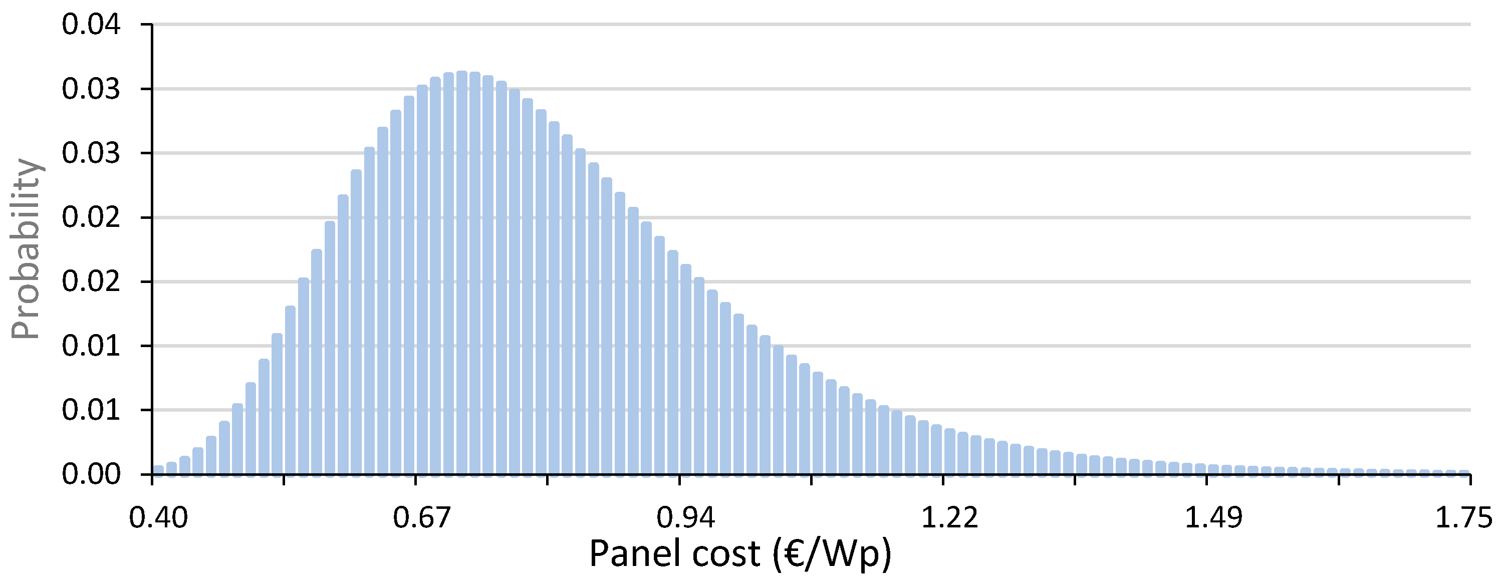
2.1.1. Solar Modules
2.1.2. Mounting Structures
2.1.3. Inverters
2.1.4. Operation and Maintenance
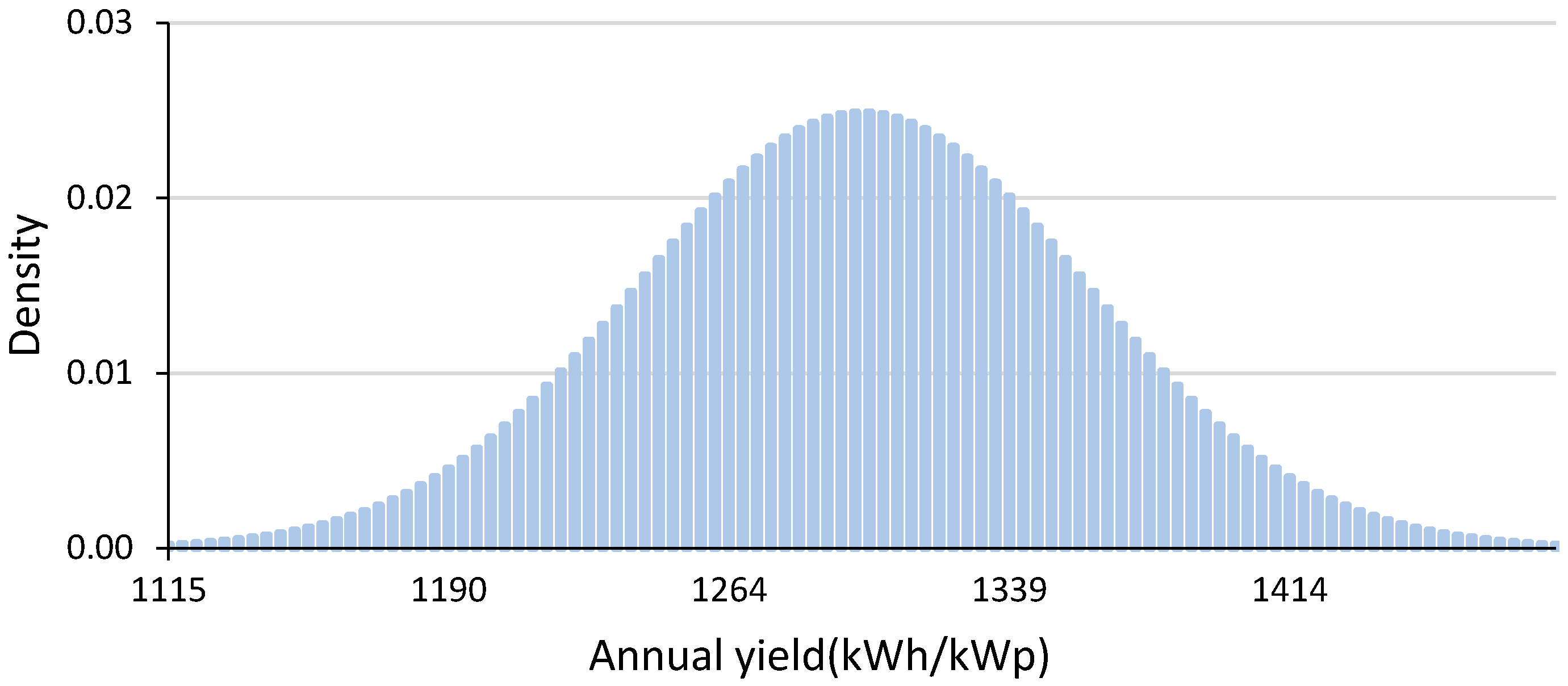
2.2. Annual Energy Production
2.3. Economic Parameters Used in the Study
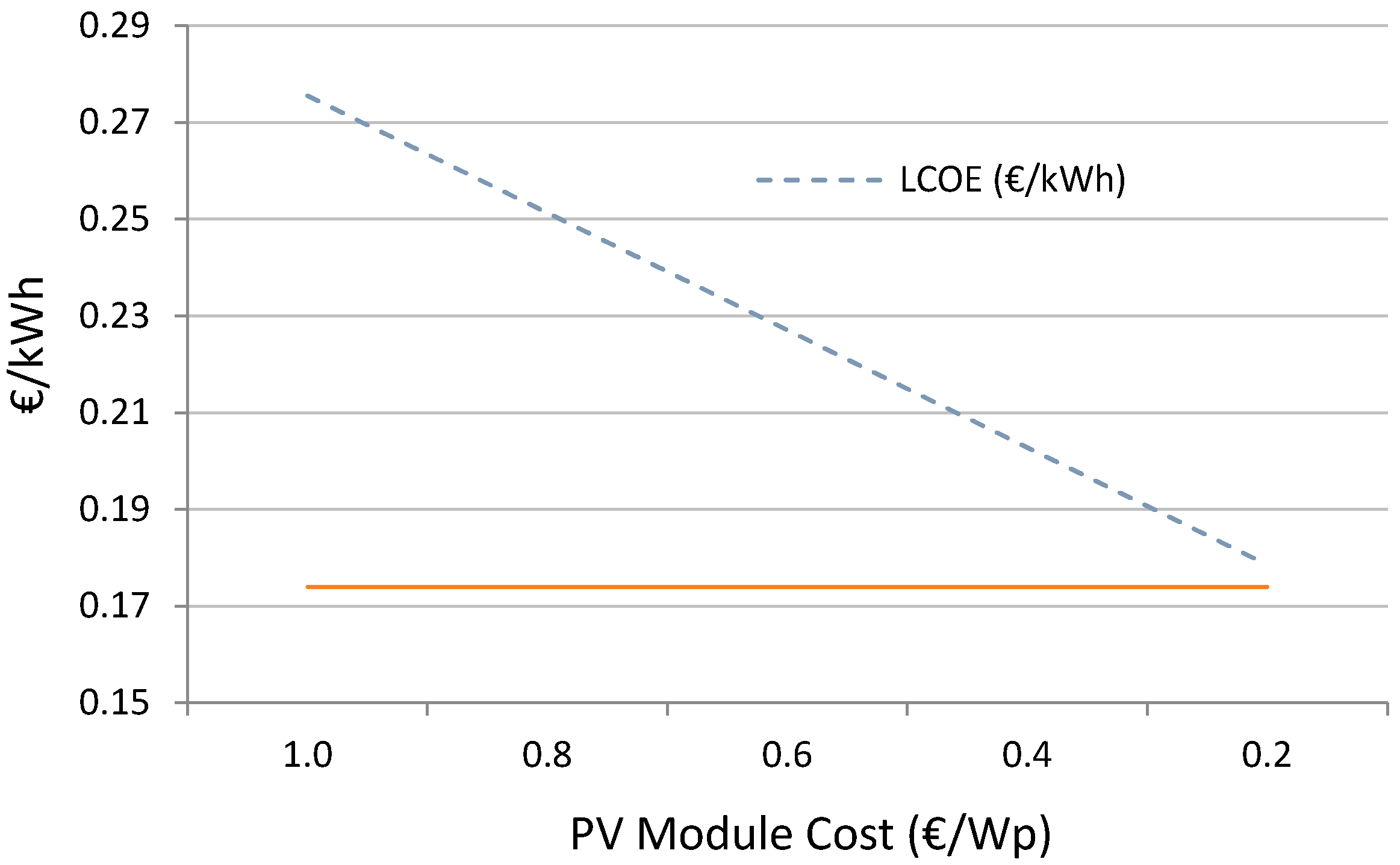
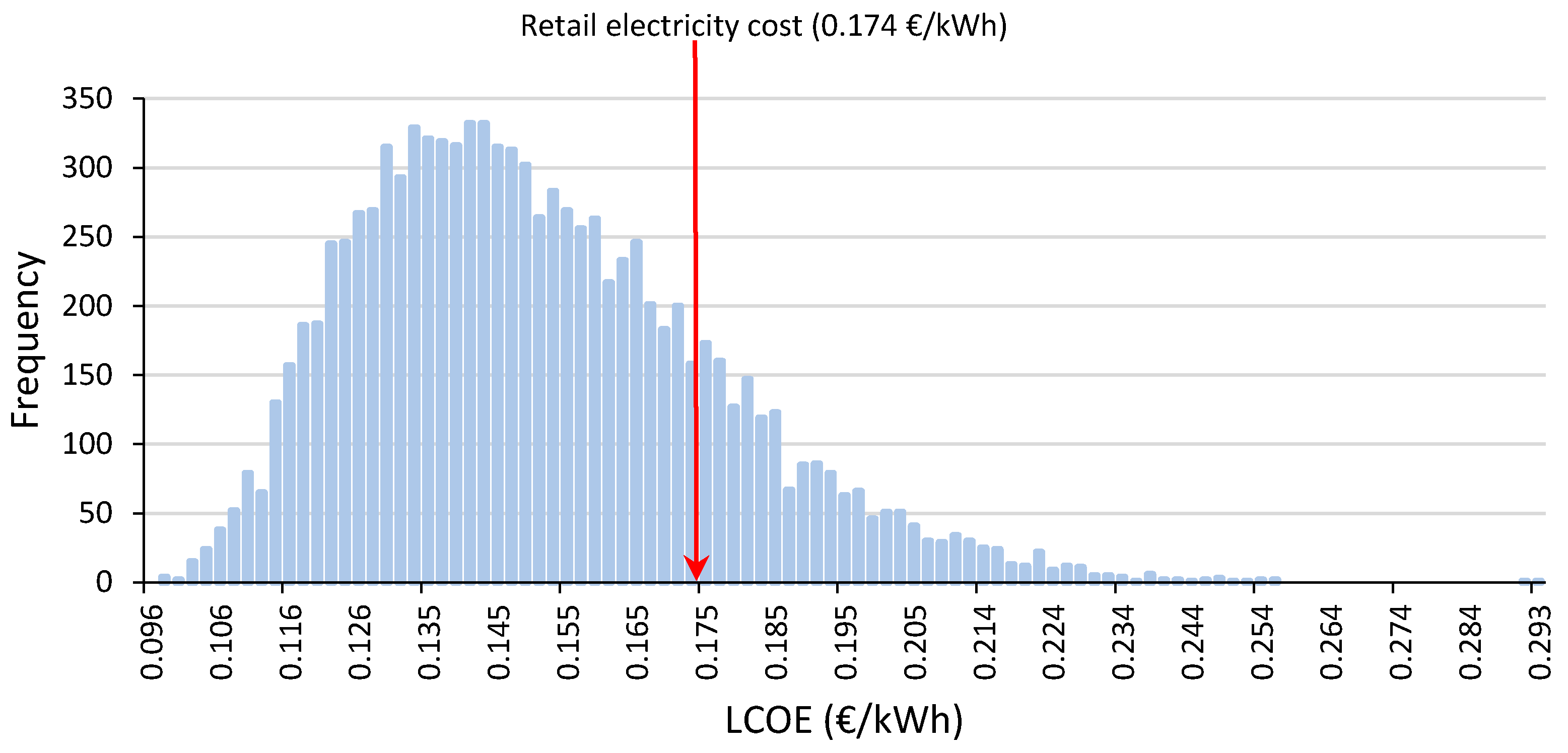
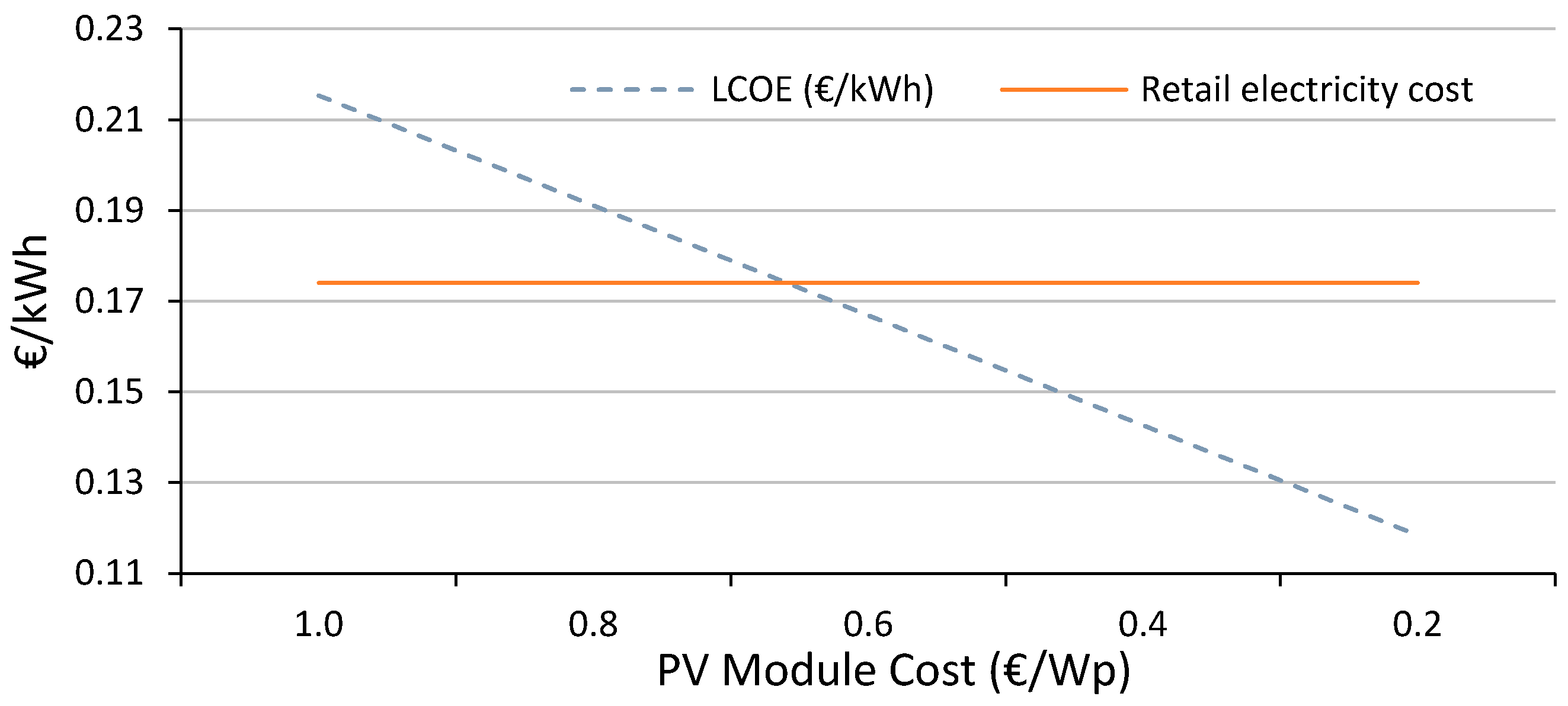
2.3.1. Levelised Cost of Energy
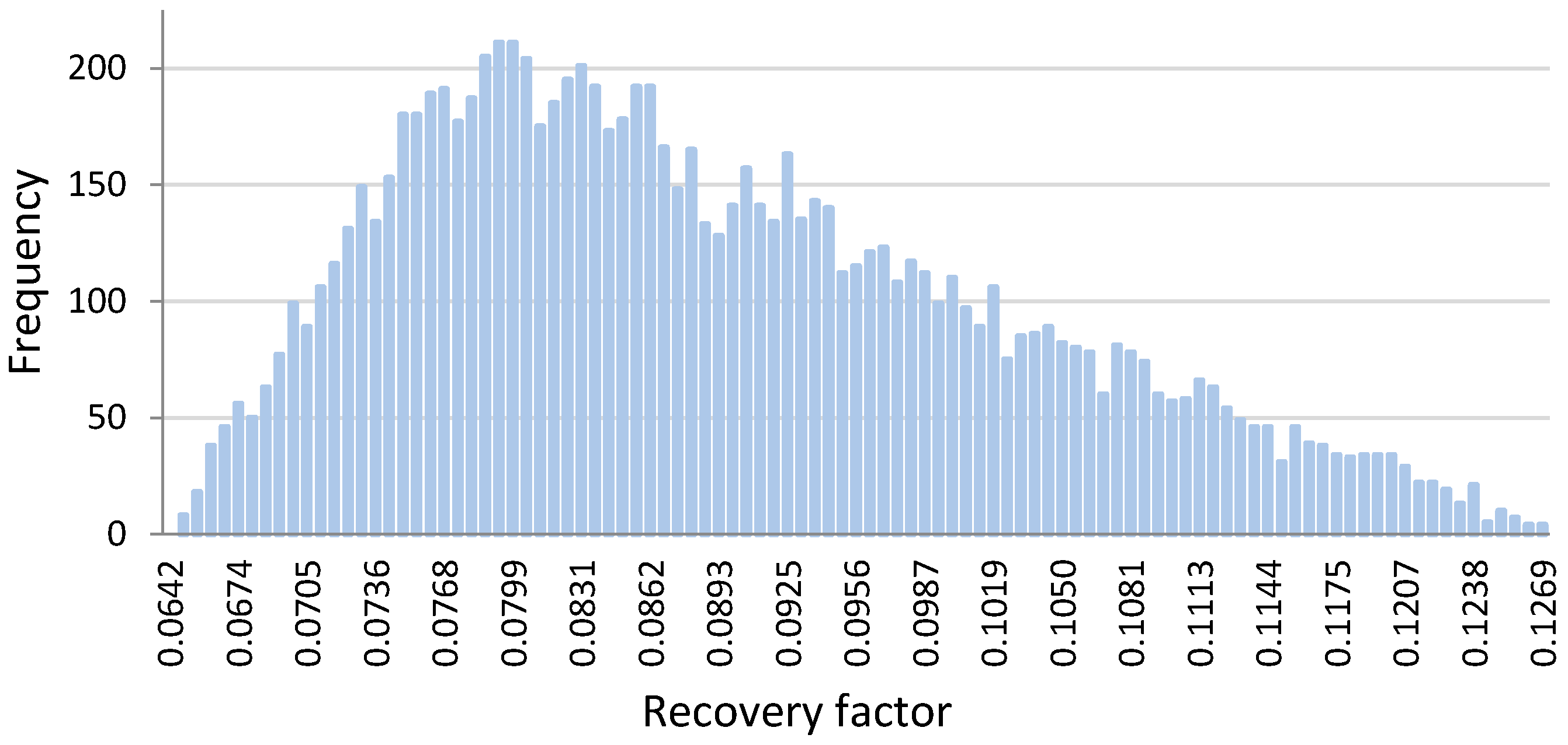
2.3.2. Capital Recovery Factor
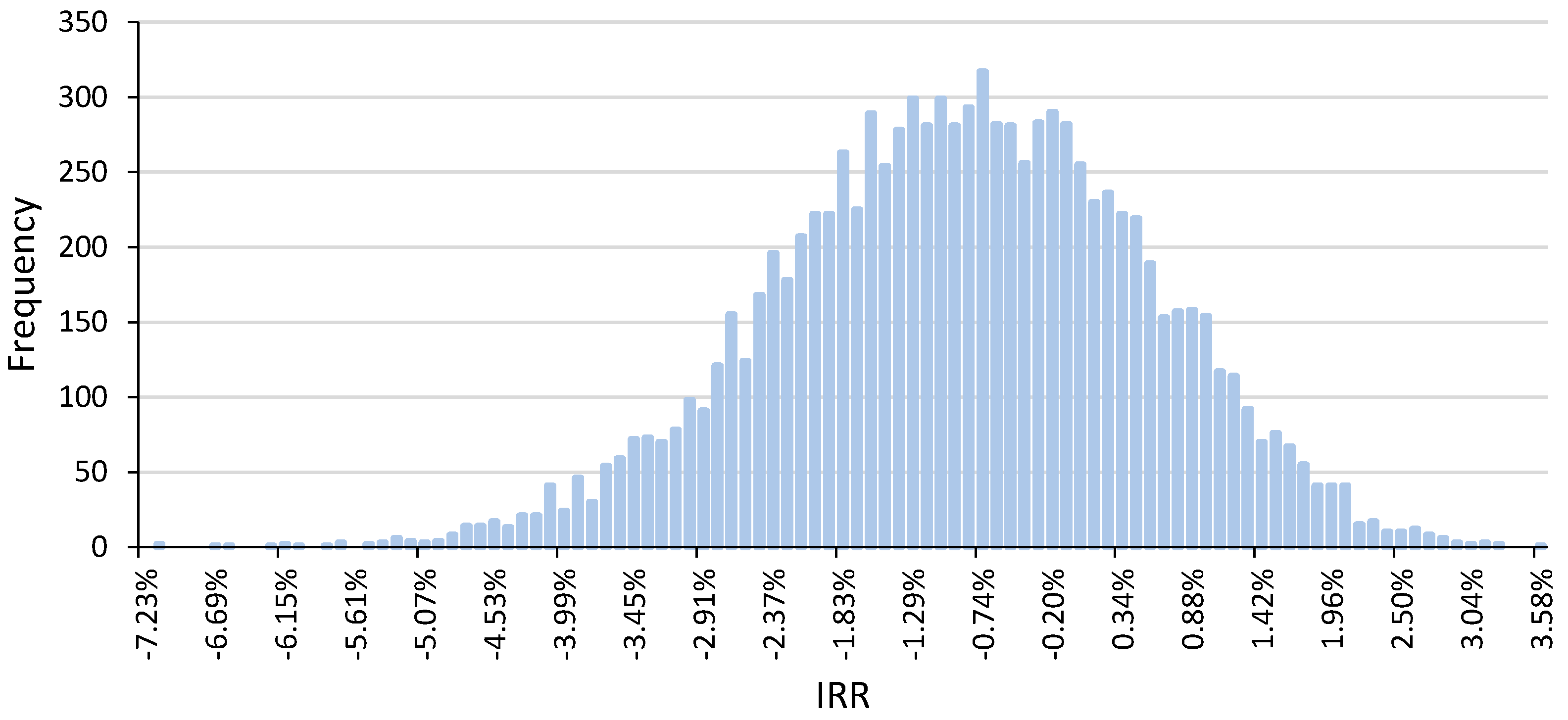
2.3.3. Internal Rate of Return
3. Results
3.1. 5 kW Case Study
3.1.1. Levelised Cost of Energy (LCOE)—Calculation Method Analysis for 5 kW and 1100 kWh/kWp Cases
3.1.2. 5 kW Case Study Sensibility Analysis
3.2. 50 kW Case Study
3.2.1. LCOE—Calculation Method Analysis for 50 kW and 1100 kWh/kWp Case
3.2.2. 50 kW Case Study Sensibility Analysis
3.3. 500 kW Case Study
3.3.1. LCOE—Calculation Method Analysis for 500 kW and 1100 kWh/kWp Case
3.3.2. 500 kW Case Study Sensibility Analysis
4. Discussion
Author Contributions
Funding
Conflicts of Interest
References and Notes
- Dufo-López, R.; Bernal-Agustín, J.L. Photovoltaic Grid Parity in Spain; Lecture Notes in Electrical Engineering; Springer: Berlin/Heidelberg, Germany, 2013; Volume 178, ISBN 9783642315275. [Google Scholar]
- Jäger-Waldau, A. PV Status Report 2014; European Commission: Luxembourg, 2014. [Google Scholar]
- Bergek, A.; Mignon, I.; Sundberg, G. Who invests in renewable electricity production? Empirical evidence and suggestions for further research. Energy Policy 2013, 56, 568–581. [Google Scholar] [CrossRef]
- Sarasa-Maestro, C.J.; Dufo-López, R.; Bernal-Agustín, J.L. Photovoltaic remuneration policies in the European Union. Energy Policy 2013, 55, 317–328. [Google Scholar] [CrossRef]
- Badcock, J.; Lenzen, M. Subsidies for electricity-generating technologies: A review. Energy Policy 2010, 38, 5038–5047. [Google Scholar] [CrossRef]
- Helms, T.; Salm, S.; Wüstenhagen, R. Investor-Specific Cost of Capital and Renewable Energy Investment Decisions. In Renewable Energy Finance; Imperical College Press: London, UK, 2015; pp. 77–101. [Google Scholar]
- Bürer, M.J.; Wüstenhagen, R. Which renewable energy policy is a venture capitalist’s best friend? Empirical evidence from a survey of international cleantech investors. Energy Policy 2009, 37, 4997–5006. [Google Scholar] [CrossRef]
- Pena-bello, A.; Burer, M.; Patel, M.K.; Parra, D. Optimizing PV and grid charging in combined applications to improve the pro fi tability of residential batteries. J. Energy Storage 2017, 13, 58–72. [Google Scholar] [CrossRef]
- Li, Y.; Gao, W.; Ruan, Y. Performance investigation of grid-connected residential PV-battery system focusing on enhancing self-consumption and peak shaving in. Renew. Energy 2018, 127, 514–523. [Google Scholar] [CrossRef]
- Nengroo, S.H.; Kamran, M.A.; Ali, M.U.; Kim, D.; Kim, M.; Hussain, A.; Kim, H.J. Dual Battery Storage System: An Optimized Strategy for the Utilization of Renewable Photovoltaic Energy in the United Kingdom. Electronics 2018, 7, 177. [Google Scholar] [CrossRef]
- Tervo, E.; Agbim, K.; Deangelis, F.; Kyung, H. An economic analysis of residential photovoltaic systems with lithium ion battery storage in the United States. Renew. Sustain. Energy Rev. 2018, 94, 1057–1066. [Google Scholar] [CrossRef]
- Royal Decree 661/2007 dated 25th of May by which the activity of production of electric energy in a special regime is regulated, Spain 2007.
- Ondraczek, J.; Komendantova, N.; Patt, A. WACC the dog: The effect of financing costs on the levelized cost of solar PV power. Renew. Energy 2015, 75, 888–898. [Google Scholar] [CrossRef]
- Branker, K.; Pathak, M.J.M.; Pearce, J.M. A review of solar photovoltaic levelized cost of electricity. Renew. Sustain. Energy Rev. 2011, 15, 4470–4482. [Google Scholar] [CrossRef]
- Szabó, S.; Jäger-Waldau, A.; Szabó, L. Risk adjusted financial costs of photovoltaics. Energy Policy 2010, 38, 3807–3819. [Google Scholar] [CrossRef]
- Geissmann, T.; Ponta, O. A probabilistic approach to the computation of the levelized cost of electricity. Energy 2017, 124, 372–381. [Google Scholar] [CrossRef]
- Tomosk, S.; Haysom, J.E.; Wright, D. Quantifying economic risk in photovoltaic power projects. Renew. Energy 2017, 109, 422–433. [Google Scholar] [CrossRef]
- Heck, N.; Smith, C.; Hittinger, E. A Monte Carlo approach to integrating uncertainty into the levelized cost of electricity. Electr. J. 2016, 29, 21–30. [Google Scholar] [CrossRef]
- Da Silver Pereira, E.J.; Pinho, J.T.; Galhardo, M.A.B.; Macêdo, W.N. Methodology of risk analysis by Monte Carlo Method applied to power generation with renewable energy. Renew. Energy 2014, 69, 347–355. [Google Scholar] [CrossRef]
- Karneyeva, Y.; Wüstenhagen, R. Solar feed-in tariffs in a post-grid parity world: The role of risk, investor diversity and business models. Energy Policy 2017, 106, 445–456. [Google Scholar] [CrossRef]
- STA, Solar Trade Association UK. Available online: http://www.solar-trade.org.uk/ (accessed on 3 November 2018).
- European Union. Commission Regulation (EU) No 182/2013 of 1 March 2013 making imports of crystalline silicon photovoltaic modules and key components. Off. J. Eur. Union 2013, 56, L152/5–L152/47. [Google Scholar]
- LME, London Metal Exchange. Available online: http://www.lme.com/ (accessed on 11 November 2018).
- United States Department of Energy. United States Energy Information Administration Updated Capital Cost Estimates for Utility Scale Electricity Generating Plants; United States Department of Energy: Washington, DC, USA, 2016; pp. 1–201. [Google Scholar]
- Fu, R.; Feldman, D.; Margolis, R. US Solar Photovoltaic System Cost Benchmark: Q1 2018; National Renewable Energy Laboratory (NREL): Golden, CO, USA, 2018. [Google Scholar]
- Hofmann, M.; Seckmeyer, G. Influence of various irradiance models and their combination on simulation results of photovoltaic systems. Energies 2017, 10, 1495. [Google Scholar] [CrossRef]
- Good, J.; Johnson, J.X. Impact of inverter loading ratio on solar photovoltaic system performance. Appl. Energy 2016, 177, 475–486. [Google Scholar] [CrossRef]
- UNE 206007-2:2014 IN Requirements for connecting to the power system. Part 2: Requirements concerning system security for installations containing inverters. 2014.
- IEEE. IEEE Standard for Interconnection and Interoperability of Distributed Energy Resources with Associated Electric Power Systems Interfaces; IEEE Standard 1547-2018 (Revision IEEE Std 1547-2003) 2018; IEEE: Piscataway, NJ, USA, 2018; pp. 1–138. [Google Scholar]
- Black, K. Business Statistics for Contemporary Decision Making, 7th ed.; John Wiley & Sons, Inc.: Kendallville, IN, USA, 2011; ISBN 978-1118024119. [Google Scholar]
- Killinger, S.; Lingfors, D.; Saint-Drenan, Y.M.; Moraitis, P.; van Sark, W.; Taylor, J.; Engerer, N.A.; Bright, J.M. On the search for representative characteristics of PV systems: Data collection and analysis of PV system azimuth, tilt, capacity, yield and shading. Sol. Energy 2018, 173, 1087–1106. [Google Scholar] [CrossRef]
- Tao, J.Y.; Finenko, A. Moving beyond LCOE: Impact of various financing methods on PV profitability for SIDS. Energy Policy 2016, 98, 749–758. [Google Scholar] [CrossRef]
- Van Sark, W.G.J.H.M.; Muizebelt, P.; Cace, J.; De Vries, A.; De Rijk, P. Grid parity reached for consumers in The Netherlands. In Proceedings of the 2012 38th IEEE Photovoltaic Specialists Conference, Austin, TX, USA, 3–8 June 2012; pp. 2462–2466. [Google Scholar]
- Montes, G.M.; Martin, E.P.; Bayo, J.A.; Garcia, J.O. The applicability of computer simulation using Monte Carlo techniques in windfarm profitability analysis. Renew. Sustain. Energy Rev. 2011, 15, 4746–4755. [Google Scholar] [CrossRef]
- Wambach, A. Payback criterion, hurdle rates and the gain of waiting. Int. Rev. Financ. Anal. 2000, 9, 247–258. [Google Scholar] [CrossRef]


| Interest rate (%) | 12 | 10 | 8 | 6 | 4 |
| Recovery factor (α) | 0.1275 | 0.1102 | 0.0937 | 0.0782 | 0.0640 |
| Inputs | Range | Unit | |
|---|---|---|---|
| Power | Constant value | 6–600 | kWp |
| Lifetime of the system | Constant value | 25 | Years |
| Annual Yield | Normal | 1100–1500 | kWh/kWp |
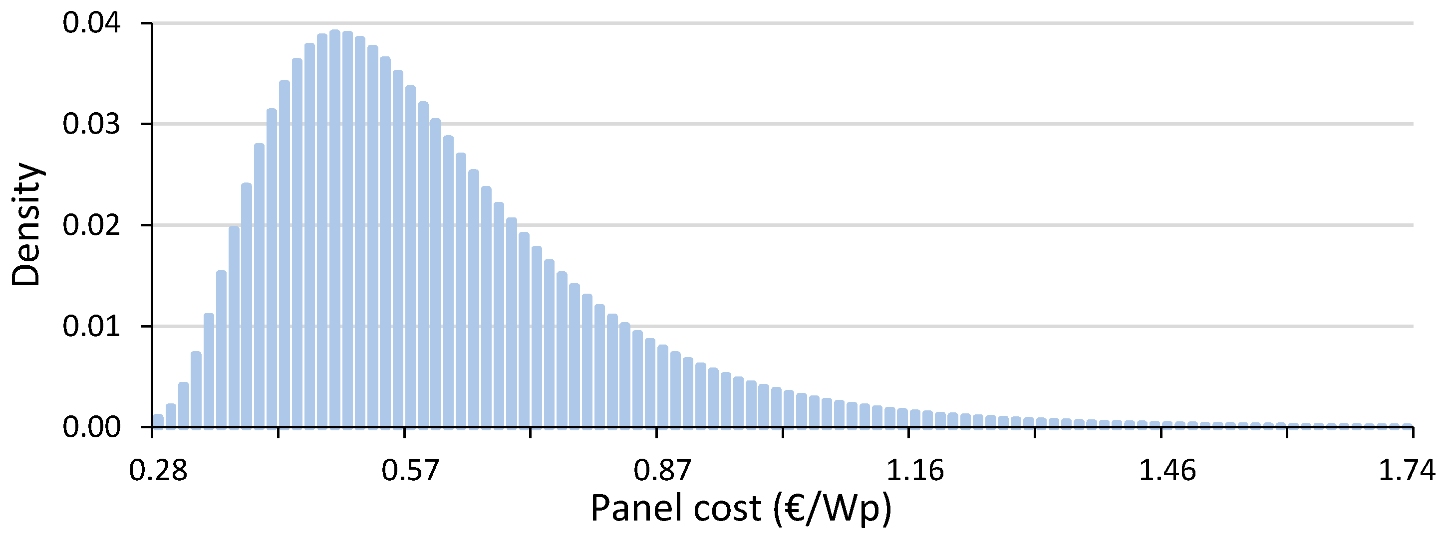
| Capital expenditure | Log-normal | 0.2–1 | €/Wp |
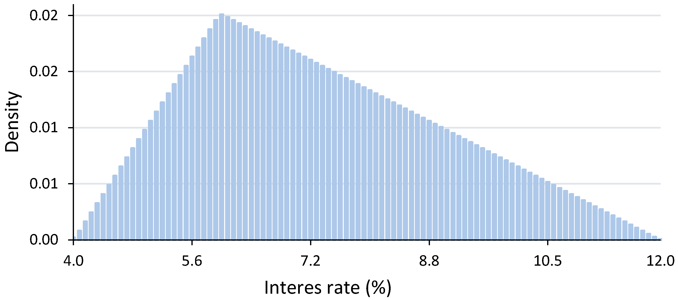
| Interest rate | Triangular | 4–12 | % |
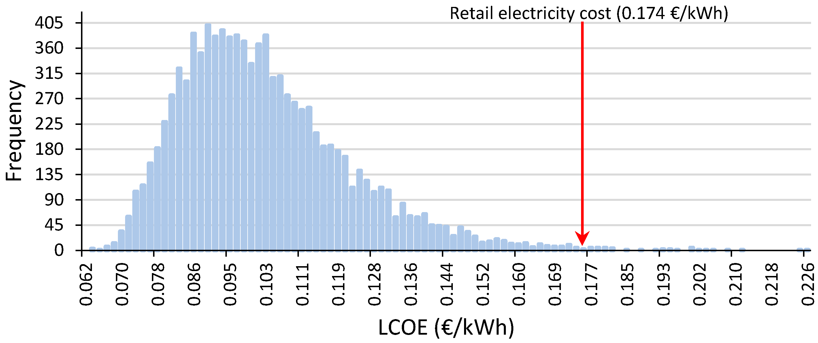
| Retail cost | Constant | 0.174 | €/kWh |
| PV Module Cost (€/Wp) | |||||
|---|---|---|---|---|---|
| 1 | 0.8 * | 0.6 | 0.4 | 0.2 | |
| PV module (6 kWp) | 6000 | 4800 | 3600 | 2400 | 1200 |
| Fixed installation costs | 6780 | 6780 | 6780 | 6780 | 6780 |
| TOTAL PV installed cost (€) | 12,780 | 11,580 | 10,380 | 9180 | 7980 |
| VAT (21%) | 2684 | 2432 | 2180 | 1928 | 1676 |
| TOTAL PV installed cost, including taxes (€) | 15,464 | 14,012 | 12,560 | 11,108 | 9656 |
| Total specific cost (€/Wp) | 2.58 | 2.34 | 2.09 | 1.85 | 1.61 |
| Total specific cost (€/W) | 3.09 | 2.80 | 2.51 | 2.22 | 1.93 |
| PV Module Cost (€/Wp) | System Cost (€) | LCOE (€/kWh) | IRR (%) |
|---|---|---|---|
| 1 | 15,464 | 0.2756 | −4.811 |
| 0.8 | 14,012 | 0.2514 | −3.83 |
| 0.6 | 12,560 | 0.2271 | −2.68 |
| 0.4 | 11,108 | 0.2029 | −1.31 |
| 0.2 | 9656 | 0.1787 | 0.40 |
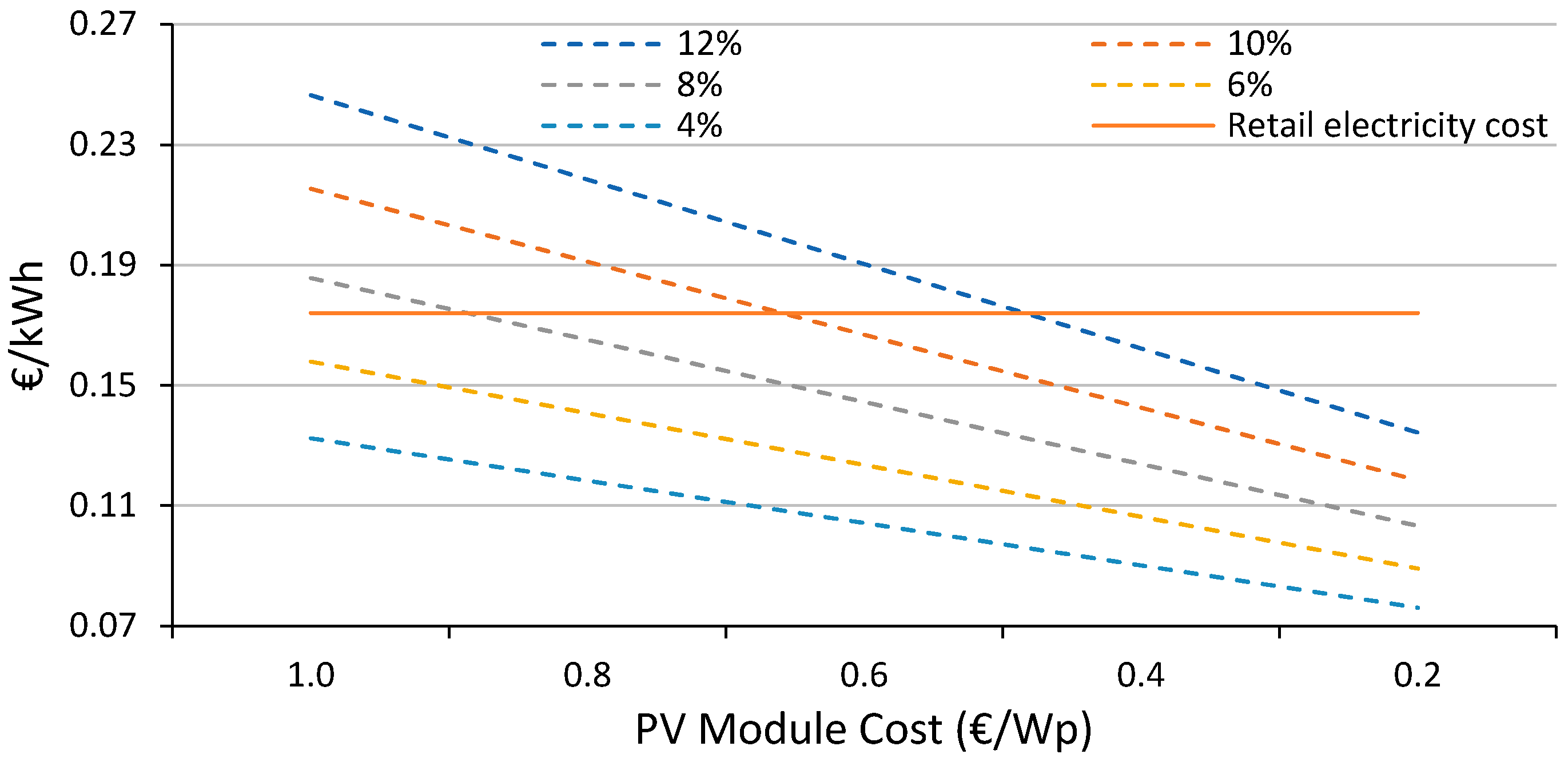
| PV Module Cost (€/Wp) | System Cost (€) | LCOE (€/kWh) | |||||
|---|---|---|---|---|---|---|---|
| Interest Rate (%): | 12 | 10 | 8 | 6 | 4 | ||
| 1.0 | 15,464 | 0.3161 | 0.2755 | 0.2369 | 0.2007 | 0.1674 | |
| 0.8 | 14,012 | 0.2881 | 0.2513 | 0.2163 | 0.1835 | 0.1533 | |
| 0.6 | 12,560 | 0.2600 | 0.2270 | 0.1957 | 0.1663 | 0.1392 | |
| 0.4 | 11,108 | 0.2320 | 0.2028 | 0.1751 | 0.1491 | 0.1251 | |
| 0.2 | 9656 | 0.2039 | 0.1786 | 0.1545 | 0.1318 | 0.1110 | |
| LCOE (€/kWh) | |||||||
|---|---|---|---|---|---|---|---|
| PV Module Cost (€/Wp) | System Cost (€) | Annual Yield (kWh/kWp): | Case 1 1100 | Case 2 1200 | Case 3 1300 | Case 4 1400 | Case 5 1500 |
| 1.0 | 15,464 | 0.276 | 0.254 | 0.236 | 0.220 | 0.207 | |
| 0.8 | 14,012 | 0.251 | 0.232 | 0.215 | 0.201 | 0.189 | |
| 0.6 | 12,560 | 0.227 | 0.210 | 0.195 | 0.182 | 0.171 | |
| 0.4 | 11,108 | 0.203 | 0.187 | 0.174 | 0.163 | 0.153 | |
| 0.2 | 9656 | 0.179 | 0.165 | 0.154 | 0.144 | 0.136 | |
| PV Module Cost (€/Wp) | |||||
|---|---|---|---|---|---|
| 1 | 0.8 | 0.6 * | 0.4 | 0.2 | |
| PV module (60 kWp) | 60,000 | 48,000 | 36,000 | 24,000 | 12,000 |
| Fixed installation costs | 38,000 | 38,000 | 38,000 | 38,000 | 38,000 |
| TOTAL PV installed cost (€) | 98,000 | 86,000 | 74,000 | 62,000 | 50,000 |
| VAT (21%) | 20,580 | 18,060 | 15,540 | 13,020 | 10,500 |
| TOTAL PV installed cost, including taxes (€) | 118,580 | 104,060 | 89,540 | 75,020 | 60,500 |
| Total specific cost (€/Wp) | 1.98 | 1.73 | 1.49 | 1.25 | 1.01 |
| Total specific cost (€/W) | 2.37 | 2.08 | 1.79 | 1.50 | 1.21 |
| PV Module Cost (€/Wp) | System Cost (€) | LCOE (€/kWh) | IRR (%) |
|---|---|---|---|
| 1 | 118,580 | 0.2154 | −2.049 |
| 0.8 | 104,060 | 0.1911 | −0.53 |
| 0.6 | 89,540 | 0.1669 | 1.39 |
| 0.4 | 75,020 | 0.1427 | 3.97 |
| 0.2 | 60,500 | 0.11841 | 7.46 |
| PV Module Cost (€/Wp) | System Cost (€) | LCOE (€/kWh) | |||||
|---|---|---|---|---|---|---|---|
| Interest Rate (%): | 12 | 10 | 8 | 6 | 4 | ||
| 1.0 | 118,580 | 0.2465 | 0.2153 | 0.1857 | 0.1579 | 0.1324 | |
| 0.8 | 104,060 | 0.2184 | 0.1911 | 0.1651 | 0.1407 | 0.1183 | |
| 0.6 | 89,540 | 0.1904 | 0.1669 | 0.1445 | 0.1235 | 0.1042 | |
| 0.4 | 75,020 | 0.1623 | 0.1426 | 0.1239 | 0.1063 | 0.0902 | |
| 0.2 | 60,500 | 0.1343 | 0.1184 | 0.1033 | 0.0891 | 0.0761 | |
| LCOE (€/kWh) | |||||||
|---|---|---|---|---|---|---|---|
| PV Module Cost (€/Wp) | System Cost (€) | Annual Yield (kWh/kWp): | Case 1 1100 | Case 2 1200 | Case 3 1300 | Case 4 1400 | Case 5 1500 |
| 1.0 | 118,580 | 0.215 | 0.199 | 0.185 | 0.173 | 0.163 | |
| 0.8 | 104,060 | 0.191 | 0.177 | 0.164 | 0.154 | 0.145 | |
| 0.6 | 89,540 | 0.167 | 0.154 | 0.144 | 0.135 | 0.127 | |
| 0.4 | 75,020 | 0.143 | 0.132 | 0.123 | 0.116 | 0.109 | |
| 0.2 | 60,500 | 0.118 | 0.110 | 0.103 | 0.097 | 0.091 | |
| PV Module Cost (€/Wp) | |||||
|---|---|---|---|---|---|
| 1 | 0.8 | 0.6 | 0.4 * | 0.2 | |
| PV module (600 kWp) | 600,000 | 480,000 | 360,000 | 240,000 | 120,000 |
| Fixed installation costs | 245,000 | 245,000 | 245,000 | 245,000 | 245,000 |
| TOTAL PV installed cost (€) | 980,000 | 725,000 | 605,000 | 485,000 | 365,000 |
| VAT (21%) | 177,450 | 152,250 | 127,050 | 101,850 | 76,650 |
| TOTAL PV installed cost, including taxes (€) | 1,022,45 | 877,250 | 732,050 | 586,850 | 441,650 |
| Total specific cost (€/Wp) | 1.70 | 1.46 | 1.22 | 0.98 | 0.74 |
| Total specific cost (€/W) | 2.04 | 1.75 | 1.46 | 1.17 | 0.88 |
| PV Module Cost (€/Wp) | System Cost (€) | LCOE (€/kWh) | IRR (%) |
|---|---|---|---|
| 1 | 1,022,45 | 0.1585 | −0.316 |
| 0.8 | 877,250 | 0.1385 | 1.67 |
| 0.6 | 732,050 | 0.1184 | 4.36 |
| 0.4 | 586,850 | 0.0984 | 8.02 |
| 0.2 | 441,650 | 0.07834 | 14.52 |
| PV Module Cost (€/Wp) | System Cost (€) | LCOE (€/kWh) | |||||
|---|---|---|---|---|---|---|---|
| Interest Rate (%): | 12 | 10 | 8 | 6 | 4 | ||
| 1.0 | 1,022,450 | 0.2149 | 0.1881 | 0.1625 | 0.1386 | 0.1166 | |
| 0.8 | 877,250 | 0.1869 | 0.1638 | 0.1419 | 0.1214 | 0.1025 | |
| 0.6 | 732,050 | 0.1588 | 0.1396 | 0.1213 | 0.1042 | 0.0884 | |
| 0.4 | 586,850 | 0.1308 | 0.1154 | 0.1007 | 0.0870 | 0.0743 | |
| 0.2 | 441,650 | 0.1027 | 0.0911 | 0.0801 | 0.0697 | 0.0602 | |
| LCOE (€/kWh) | |||||||
|---|---|---|---|---|---|---|---|
| PV Module Cost (€/Wp) | System Cost (€) | Annual Yield (kWh/kWp): | Case 1 1100 | Case 2 1200 | Case 3 1300 | Case 4 1400 | Case 5 1500 |
| 1.0 | 1,022,450 | 0.188 | 0.174 | 0.162 | 0.151 | 0.143 | |
| 0.8 | 877,250 | 0.164 | 0.152 | 0.141 | 0.132 | 0.125 | |
| 0.6 | 732,050 | 0.140 | 0.129 | 0.121 | 0.113 | 0.107 | |
| 0.4 | 586,850 | 0.115 | 0.107 | 0.100 | 0.094 | 0.089 | |
| 0.2 | 441,650 | 0.118 | 0.110 | 0.103 | 0.097 | 0.091 | |
| PV Module Cost (€/Wp) | LCOE (€/kWh) | ||
|---|---|---|---|
| 5 kW | 50 kW | 500 kW | |
| 1 | 0.2756 | 0.2154 | 0.1585 |
| 0.8 | 0.2514 | 0.1911 | 0.1385 |
| 0.6 | 0.2271 | 0.1669 | 0.1184 |
| 0.4 | 0.2029 | 0.1427 | 0.0984 |
| 0.2 | 0.1787 | 0.1184 | 0.0783 |
| PV Module Cost (€/Wp) | IRR (%) | ||
|---|---|---|---|
| 5 kW | 50 kW | 500 kW | |
| 1 | −4.81 | −2.05 | −0.32 |
| 0.8 | −3.83 | −0.53 | 1.67 |
| 0.6 | −2.68 | 1.39 | 4.36 |
| 0.4 | −1.31 | 3.97 | 8.02 |
| 0.2 | 0.40 | 7.46 | 14.52 |
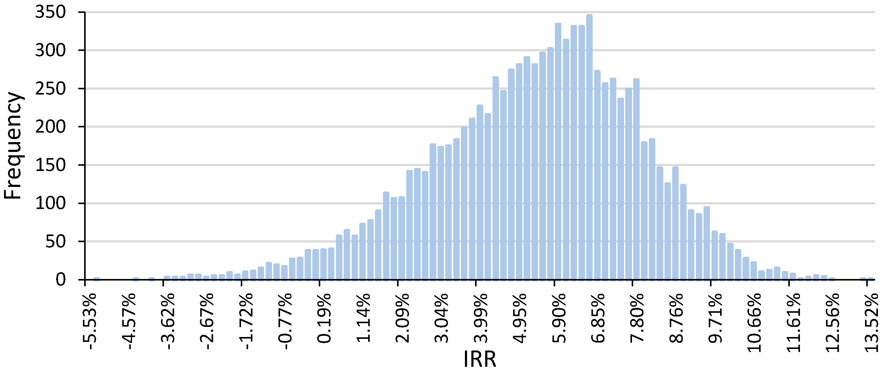
| Power (kW) | Mean PV Module Cost (€/Wp) | Mean Yield (kWh/kWp) | Mean Interest Rate (%) | Mean LCOE (€/kWh) | Mean IRR (%) | Success Rate (%) |
|---|---|---|---|---|---|---|
| 5 | 0.8 | 1300 | 6 | 0.1494 | −0.97 | 82.26 |
| 50 | 0.6 | 1300 | 6 | 0.1019 | 5.92 | 99.59 |
| 500 | 0.4 | 1300 | 6 | 0.0727 | 14.34 | 99.80 |
© 2019 by the authors. Licensee MDPI, Basel, Switzerland. This article is an open access article distributed under the terms and conditions of the Creative Commons Attribution (CC BY) license (http://creativecommons.org/licenses/by/4.0/).
Share and Cite
Sarasa-Maestro, C.J.; Dufo-López, R.; Bernal-Agustín, J.L. Evaluating the Effect of Financing Costs on PV Grid Parity by Applying a Probabilistic Methodology. Appl. Sci. 2019, 9, 425. https://doi.org/10.3390/app9030425
Sarasa-Maestro CJ, Dufo-López R, Bernal-Agustín JL. Evaluating the Effect of Financing Costs on PV Grid Parity by Applying a Probabilistic Methodology. Applied Sciences. 2019; 9(3):425. https://doi.org/10.3390/app9030425
Chicago/Turabian StyleSarasa-Maestro, Carlos J., Rodolfo Dufo-López, and José L. Bernal-Agustín. 2019. "Evaluating the Effect of Financing Costs on PV Grid Parity by Applying a Probabilistic Methodology" Applied Sciences 9, no. 3: 425. https://doi.org/10.3390/app9030425
APA StyleSarasa-Maestro, C. J., Dufo-López, R., & Bernal-Agustín, J. L. (2019). Evaluating the Effect of Financing Costs on PV Grid Parity by Applying a Probabilistic Methodology. Applied Sciences, 9(3), 425. https://doi.org/10.3390/app9030425