Optimization of Optical Networks Based on CDC-ROADM Technology

Abstract

New generation of optical nodes in dense wavelength division multiplexed networks enables operators to improve service flexibility and make significant savings, both in operational and capital expenditures. Thus the main objective of the study is to minimize optical node resources, such as transponders, multiplexers and wavelength selective switches, needed to provide and maintain high quality dense wavelength division multiplexed network services using new generation of optical nodes. A model based on integer programming is proposed, which includes a detailed description of an optical network node. The impact on the network performance of conventional reconfigurable optical add drop multiplexer technology is compared with colorless, directionless and contentionless approaches. The main focus of the presented study is the analysis of the network congestion problem arising in the context of both reconfigurable optical add drop multiplexer technologies. The analysis is supported by results of numerical experiments carried out for realistic networks of different dimensions and traffic demand sets.

1. Introduction

Colorless, Directionless and Contentionless Reconfigurable Optical Add Drop Multiplexers (CDC-ROADMs) have become an important element of optical transmission systems deployed by major network operators across the world. This is because Conventional Reconfigurable Optical Add Drop Multiplexers (C-ROADMs) fail to provide wavelength routing flexibility sufficient to meet system requirements resulting from rapid data traffic growth in optical networks [1] (CDC) [2,3,4]. 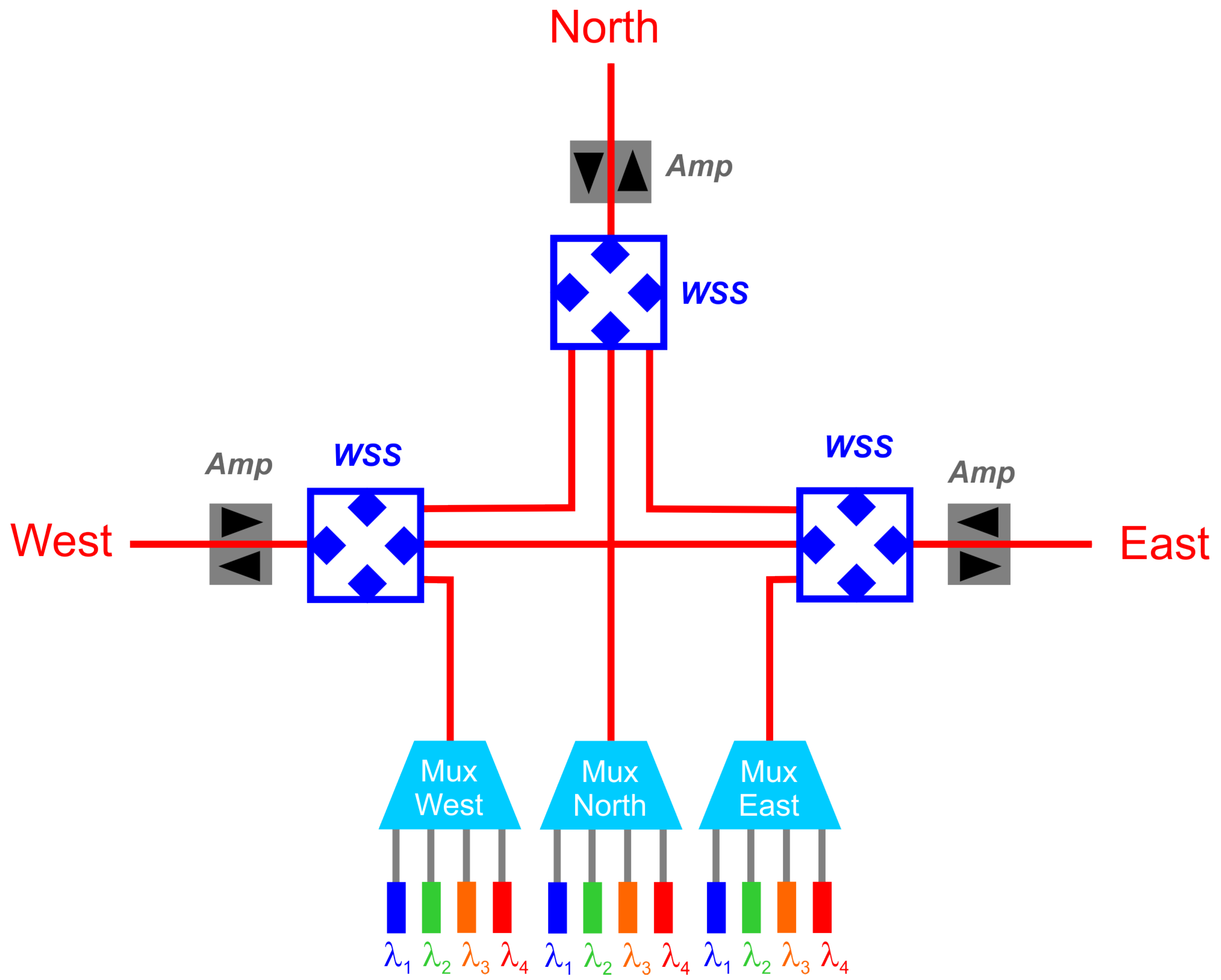Figure 1 shows a schematic diagram of C-ROADM. C-ROADMs are limited by fixed wavelength assignment to specific ports and fixed direction assignment for multiplexers and thus can add/drop a wavelength only to a fixed outgoing direction. For instance, in Figure 1 a transponder connected to the Mux West can only add/drop a wavelength to the West direction and not to any other (i.e., North or East). Thus rerouting the wavelength emitted by a transponder connected to Mux West to a different direction requires a visit of an engineer on site in order to manually connect the transponder to the correct mux/demux port. Hence, C-ROADM technology is also incompatible with the concept of the software defined network (SDN). On the positive side C-ROADM architectures, based on Wavelength Selective Switch (WSS), allow for simple adding, dropping and express routing traffic through network nodes and hence offer benefits such as simple planning, simple and robust bandwidth use and low cost network maintenance. Nonetheless, the growing traffic in optical networks renders C-ROADM technology more and more obsolete due to their low routing flexibility and lack of ability to conform with SDN paradigm.

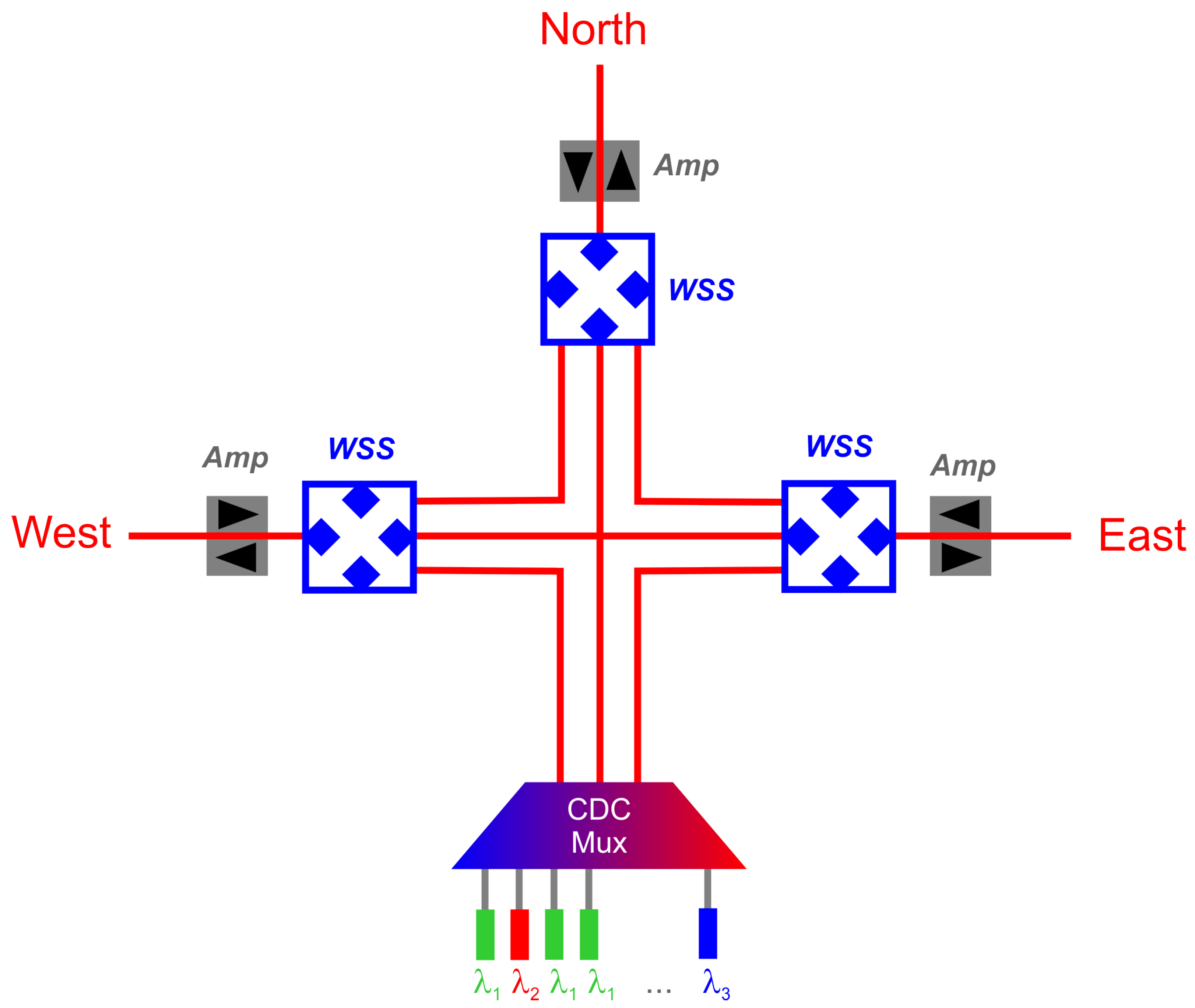
CDC-ROADMs are of great interest to next generation optical telecom networks since they offer much greater wavelength routing flexibility than C-ROADMs and also because they conform with the SDN paradigm. Figure 2 shows a schematic diagram of a CDC-ROADM. Using CDC-ROADMs optical network operators can remotely connect any wavelength from any transponder to any direction (Figure 2). Thus regardless of specific architecture details, the final result is that any wavelength (color) can be assigned to any port at the add/drop site, using remote software control without any technician intervention on site [5,6]. This combined with now widely deployed remotely tunable coherent transponders gives a network operator unprecedented capability to manage the optical network within the SDN paradigm thus enhancing network flexibility and survivability while reducing capital and operational expenses. This is because with tunable transponders network operators do not need to pay high capital expense by installing transponders for all wavelengths, but can implement an investment strategy of “pay as you grow”.

It is noted that there are also intermediate optical node architectures between C-ROADM and CDC-ROADM. Colorless ROADM node architectures can remotely assign any wavelength to a particular Mux port and thus provide the means for building ROADMs that automate the assignment of add/drop wavelengths. Additionally, having colorless functionality, one can use different wavelengths for different sections in the optical path to avoid congestion in the network. Directionless ROADMs, by contrast, allow any wavelength to be routed to any direction served by a node using software control without any physical rewiring. Colorless and directionless ROADMs combine the advantages of both technologies [6,7,8]. However, even with colorless and directionless functionality, an optical network still has limitations that could require manual intervention on site in some cases. In other words, the colorless, directionless network is still not completely flexible and compatible with the SDN concept. Only a contentionless architecture, allows multiple copies of the same wavelength on a single add/drop Mux. Thus only a colorless, directionless architecture combined with contentionless functionality is the end goal of any network operator that has deployed or is planning to deploy ultimate level of flexibility in the optical layer [9] especially together with flexible wavelength assignment [4,10]. Further, the advantages of CDC-ROADMs enable operators to offer a flexible service and provide significant savings in Operational Expenditure (OpEx) and Capital Expenditure (CapEx). OpEx reductions are delivered primarily by means of touchless provisioning and activation of network bandwidth. Finally, it is noted that another important problem arises from the need for manual provisioning in C-ROADM systems since it makes them vulnerable to a possibility of human errors. Obviously, with CDC-ROADMs, the risk resulting from human error is significantly reduced because of fully automated provisioning.

During the last decade, the attention of the telecommunication community has been concentrated on Routing and Wavelength Assignment (RWA) and Routing and Spectrum Allocation (RSA) problems. Consequently, numerous exact and heuristic methods are now available to solve RWA and RSA problems in static [9,10,11] and dynamic [12,13,14] environment. However, so far the relevance of the inner optical node architecture in the DWDM network optimization has not been fully considered. In [15] a detailed node cost model has been presented. However, the authors did not focus on optimization. There are works dealing with single aspects of the node architecture optimization problem [16]. However, the complete picture has not yet been presented. This study concentrates on the optical node structure and its relevance in DWDM network resources optimization by taking into account various types of transponders, multiplexers (filters, which differ for various technologies) and wavelength selective switches [3]. The problem is formulated using Mixed Integer Programming (MIP). A comparative study of C-ROADM and CDC-ROADM node network is performed. Network topologies are realistic and represent optical DWDM networks from selected countries [17]. Traffic demands are typical for DWDM networks and are represented using a traffic matrix.

The rest of the paper is organized as follows. After introduction, in the second section the model details for various technologies are provided. In the third section a discussion of the results is provided, which is followed by a concise summary given in the last section.

2. Methods

In this section DWDM network optimization problem is formulated using MIP. For this purpose the following sets are defined: $\mathcal{N}$ the set of all nodes; $\mathcal{T}$ the set of transponders; $\mathcal{P}$ the set of time periods; $\mathcal{S}$ the set of frequency slices; $\mathcal{E}$ the set of edges; ${\delta }^{+}(n)$ the set of edges starting at node n, and ${\delta }^{-}(n)$ the set of edges ending at node n.

The following objective cost function is optimized using an IP algorithm subject to the listed below constraints:

$$\begin{array}{c}\hfill min\sum _{p\in \mathcal{P}}\sum _{n\in \mathcal{N}}(w_{np}\xi (n)+\sum _{t\in \mathcal{T}}{x}_{tnp}\xi (t))\end{array}$$

(1a)

$$\begin{array}{c}\hfill \sum _{n^{\prime }\in \mathcal{N}}{z}_{n^{″}p}^{(n,n^{\prime })}=\sum _{n^{\prime }\in \mathcal{N}}{z}_{n^{″}p}^{(n^{\prime },n)}+h(n,n^{″},p)\forall n,n^{″}\in \mathcal{N}:n\ne n^{″},\forall p\in \mathcal{P}\end{array}$$

(1b)

$$\begin{array}{c}\hfill \sum _{s\in \mathcal{S}}\sum _{t\in \mathcal{T}}{y}_{tsp}^{(n,n^{\prime })}b(t)\ge \sum _{n^{″}\in \mathcal{N}}{z}_{n^{″}p}^{(n,n^{\prime })}\forall n,n^{\prime }\in \mathcal{N},\forall p\in \mathcal{P}\end{array}$$

(1c)

$$\begin{array}{c}\hfill g_{tsnp}\ge \sum _{n^{\prime }\in \mathcal{N}}(y_{tsp}^{(n,n^{\prime })}+y_{tsp}^{(n^{\prime },n)})\forall t\in \mathcal{T},\forall n\in \mathcal{N},\forall p\in \mathcal{P},\forall s\in \mathcal{S}\end{array}$$

(1d)

$$\begin{array}{c}\hfill x_{tnp}o(t)\ge \sum _{s\in \mathcal{S}}{g}_{tsnp}\forall t\in \mathcal{T},\forall n\in \mathcal{N},\forall p\in \mathcal{P}\end{array}$$

(1e)

$$\begin{array}{c}\hfill w_{np}M\ge \sum _{s\in \mathcal{S}}(g_{tsnp}-g_{tsnp(p)})\forall n\in \mathcal{N},\forall p\in \mathcal{P}:p(p)\ne \varnothing ,\forall t\in \mathcal{T}\end{array}$$

(1f)

$$\begin{array}{c}\hfill w_{np}M\ge \sum _{s\in \mathcal{S}}(g_{tsnp(p)}-g_{tsnp})\forall n\in \mathcal{N},\forall p\in \mathcal{P}:p(p)\ne \varnothing ,\forall t\in \mathcal{T}\end{array}$$

(1g)

$$\begin{array}{c}\hfill w_{np}M\ge \sum _{s\in \mathcal{S}}(g_{tsnp}-i(t,s,n))\forall n\in \mathcal{N},\forall p\in \mathcal{P}:p(p)=\varnothing ,\forall t\in \mathcal{T}\end{array}$$

(1h)

$$\begin{array}{c}\hfill w_{np}M\ge \sum _{s\in \mathcal{S}}(i(t,s,n)-g_{tsnp})\forall n\in \mathcal{N},\forall p\in \mathcal{P}:p(p)=\varnothing ,\forall t\in \mathcal{T}\end{array}$$

(1i)

In (1a)–(1i) we are provided with the following constants: $o(t)$ is the number of outputs of transponder t; $b(t)$ is the bitrate of one output of transponder t; $\xi (t)$ is the cost of using transponder t in one period; $h(n,n^{\prime },p)$ is the volume of demand from node n to node $n^{\prime }$ in period p; $\xi (n)$ is the cost of intervention in node n; $p(p)$ is the period before period p; p is the first period if $p(p)=\varnothing$; $i(t,s,n)$ is the number of ports of transponders t working on slice s installed in node n at time zero and M is a large number.

In the formulation we use the following variables: $x_{tnp}$ is the number of transponders t installed in node n in period p; $z_{n^{″}p}^{(n,n^{\prime })}$ is the bitrate in relation $(n,n^{\prime })$ with node $n^{″}$ being the final destination in period p; $w_{np}$ is a binary variable and equal to 1 if intervention is needed in node n in period p; $g_{tsnp}$ is the number of ports of transponders t working on slice s installed in node n in period p, and $y_{tsp}^{(n,n^{\prime })}$ is the number of outputs of transponder t working on slice s installed in relation $(n,n^{\prime })$ in period p.

Minimizing the objective function (1a) is equivalent to minimization of the total costs of interventions and transponder purchases. Constraint (1b) imposes the Kirchhoff law for traffic entering and leaving node n. Constraint (1c) assures that flow between nodes n and $n^{\prime }$ is realized using only available outputs of transponders. Constraint (1d) assures that all used outputs of transponders have corresponding ports installed. Constraint (1e) assures that all ports are installed in transponders. Constraints (1f)–(1i) assure that changing the number of active transponders requires an intervention of an engineer on site.

In case of C-ROADM several additional constraints need to be included. If we do not provide the contentionless features in the node model the following constraint should be satisfied:

$$\begin{array}{c}\hfill \sum _{t\in \mathcal{T}}{g}_{tsnp}\le 1\forall s\in \mathcal{S},\forall n\in \mathcal{N},\forall p\in \mathcal{P}\end{array}$$

(2a)

To model the C-ROADM node, additionally we must consider the following constraints, specifically related to the colored node model:

$$\begin{array}{c}\hfill w_{np}M\ge g_{tsnp}-g_{tsnp(p)}\forall n\in \mathcal{N},\forall p\in \mathcal{P}:p(p)\ne \varnothing ,\forall t\in \mathcal{T},\forall s\in \mathcal{S}\end{array}$$

(3a)

$$\begin{array}{c}\hfill w_{np}M\ge g_{tsnp(p)}-g_{tsnp}\forall n\in \mathcal{N},\forall p\in \mathcal{P}:p(p)\ne \varnothing ,\forall t\in \mathcal{T},\forall s\in \mathcal{S}\end{array}$$

(3b)

$$\begin{array}{c}\hfill w_{np}M\ge g_{tsnp}-i(t,s,n)\forall n\in \mathcal{N},\forall p\in \mathcal{P}:p(p)=\varnothing ,\forall t\in \mathcal{T},\forall s\in \mathcal{S}\end{array}$$

(3c)

$$\begin{array}{c}\hfill w_{np}M\ge i(t,s,n)-g_{tsnp}\forall n\in \mathcal{N},\forall p\in \mathcal{P}:p(p)=\varnothing ,\forall t\in \mathcal{T},\forall s\in \mathcal{S}\end{array}$$

(3d)

These constraints are stronger than (1f)–(1i) and assure that any change of colors requires an engineer intervention on site. General constraints that should be added to have directioned node model are:

$$\begin{array}{c}\hfill \sum _{e\in {\delta }^{+}(n)}{f}_{tspe}^{(n,n^{\prime })}=y_{tsp}^{(n,n^{\prime })}\forall n,n^{\prime }\in \mathcal{N},\forall t\in \mathcal{T},\forall s\in \mathcal{S},\forall p\in \mathcal{P}\end{array}$$

(4a)

$$\begin{array}{c}\hfill \sum _{e\in {\delta }^{-}(n^{\prime })}{l}_{tspe}^{(n,n^{\prime })}=y_{tsp}^{(n,n^{\prime })}\forall n,n^{\prime }\in \mathcal{N},\forall t\in \mathcal{T},\forall s\in \mathcal{S},\forall p\in \mathcal{P}\end{array}$$

(4b)

$$\begin{array}{c}\hfill g_{tsnpe}\ge \sum _{n^{\prime }\in \mathcal{N}}(f_{tspe}^{(n,n^{\prime })}+l_{tspr(e)}^{(n^{\prime },n)})\forall t\in \mathcal{T},\forall n\in \mathcal{N},\forall p\in \mathcal{P},\forall s\in \mathcal{S},\forall e\in {\delta }^{+}(n)\end{array}$$

(4c)

$$\begin{array}{c}\hfill g_{tsnp}\ge \sum _{e\in {\delta }^{+}(n)}{g}_{tsnpe}\forall n\in \mathcal{N},\forall p\in \mathcal{P},\forall t\in \mathcal{T},\forall s\in \mathcal{S}\end{array}$$

(4d)

$$\begin{array}{c}\hfill w_{np}M\ge g_{tsnpe}-g_{tsnp(p)e}\forall n\in \mathcal{N},\forall p\in \mathcal{P}:p(p)\ne \varnothing ,\forall t\in \mathcal{T},\forall s\in \mathcal{S},\forall e\in {\delta }^{+}(n)\end{array}$$

(4e)

$$\begin{array}{c}\hfill w_{np}M\ge g_{tsnp(p)e}-g_{tsnpe}\forall n\in \mathcal{N},\forall p\in \mathcal{P}:p(p)\ne \varnothing ,\forall t\in \mathcal{T},\forall s\in \mathcal{S},\forall e\in {\delta }^{+}(n)\end{array}$$

(4f)

$$\begin{array}{c}\hfill w_{np}M\ge g_{tsnpe}-i(t,s,n,e)\forall n\in \mathcal{N},\forall p\in \mathcal{P}:p(p)=\varnothing ,\forall t\in \mathcal{T},\forall s\in \mathcal{S},\forall e\in {\delta }^{+}(n)\end{array}$$

(4g)

$$\begin{array}{c}\hfill w_{np}M\ge i(t,s,n,e)-g_{tsnpe}\forall n\in \mathcal{N},\forall p\in \mathcal{P}:p(p)=\varnothing ,\forall t\in \mathcal{T},\forall s\in \mathcal{S},\forall e\in {\delta }^{+}(n)\end{array}$$

(4h)

In (4a)–(4h) we use constants $i(t,s,n,e)$, which represent the number of ports of transponders of type t in node n using slice s and edge e as the first edge at time zero.

Additionally, we use the following variables: $f_{tspe}^{(n,n^{\prime })}$ is the number of outputs of transponder t working on slice s installed in relation $(n,n^{\prime })$ in period p using edge e as the first edge; $l_{tspe}^{(n,n^{\prime })}$ is the number of outputs of transponder t working on slice s installed in relation $(n,n^{\prime })$ in period p using edge e as the last edge; $g_{tsnpe}$ is the number of ports of transponders t working on slice s installed in node n in period p using edge e as the first edge.

Constraints (4a) and (4b) assures that each allocated path defines its first and last edge, respectively. Constraint (4c) assures that there are enough appropriately directed transponder ports in each node to support allocated paths. Constraint (4d) assures that there are enough installed transponders to support all needed directions. Constraints (4e)–(4h) are stronger than (3) and assure that any change of either directions or colors requires an intervention on site.

Two types of IP DWDM optical network optimization with respect to routing paths are considered: node-link and path-link formulation. If a node-link formulation is considered the following constraints need to be added:

$$\begin{array}{c}\hfill \sum _{e\in {\delta }^{+}(n)}{k}_{sept}^{(n^{\prime },n^{″})}-\sum _{e\in {\delta }^{-}(n)}{k}_{sept}^{(n^{\prime },n^{″})}=0\forall n,n^{\prime },n^{″}\in \mathcal{N}:n\ne n^{\prime }\wedge n\ne n^{″},\forall s\in \mathcal{S},\forall p\in \mathcal{P},\forall t\in \mathcal{T}\end{array}$$

(5a)

$$\begin{array}{c}\hfill \sum _{e\in {\delta }^{+}(n)}{k}_{sept}^{(n,n^{\prime })}-\sum _{e\in {\delta }^{-}(n)}{k}_{sept}^{(n,n^{\prime })}=y_{tsp}^{(n,n^{\prime })}\forall n,n^{\prime }\in \mathcal{N},\forall s\in \mathcal{S},\forall p\in \mathcal{P},\forall t\in \mathcal{T}\end{array}$$

(5b)

$$\begin{array}{c}\hfill \sum _{n,n^{\prime }\in \mathcal{N}}\sum _{t\in \mathcal{T}}(k_{sept}^{(n,n^{\prime })}+k_{sr(e)pt}^{(n,n^{\prime })})\le 1\forall s\in \mathcal{S},\forall e\in \mathcal{E},\forall p\in \mathcal{P}\end{array}$$

(5c)

In (5a)–(5c) $r(e)$ is the edge opposite to edge e, $k_{sept}^{(n,n^{\prime })}$ is a binary variable and equal to 1 if slice s is occupied on edge e in period p by a transmission between nodes n and $n^{\prime }$ using transponder t and 0, otherwise. Constraint (5a) expresses the Kirchhoff law for all nodes that are neither source nor sink nodes of a demand. Constraint (5b) expresses the Kirchhoff law for source nodes of demands. Constraint (5c) assures that the bandwidth is reserved for both directions.

Link-path formulation is well known and often used in the literature [11,18]. For this method sets ${\mathcal{G}}_{(n,n^{\prime })}$ of all paths between nodes n and $n^{\prime }$ should be defined and the following constraints added:

$$\begin{array}{c}\hfill \sum _{g\in {\mathcal{G}}_{(n,n^{\prime })}}{k}_{sgpt}=y_{tsp}^{(n,n^{\prime })}\forall n,n^{\prime }\in \mathcal{N},\forall s\in \mathcal{S},\forall p\in \mathcal{P},t\in \mathcal{T}\end{array}$$

(6a)

$$\begin{array}{c}\hfill \sum _{n,n^{\prime }\in \mathcal{N}}\sum _{g\in {\mathcal{G}}_{(n,n^{\prime })}}\sum _{t\in \mathcal{T}}u(g,e)k_{sgpt}\le 1\forall s\in \mathcal{S},\forall e\in \mathcal{E},\forall p\in \mathcal{P}\end{array}$$

(6b)

In (6a) and (6b) ${\mathcal{G}}_{(n,n^{\prime })}$ is the paths set between nodes n and $n^{\prime }$; $u(g,e)$ is a binary constant and equal to 1 if path g uses edges e or $r(e)$ and equal to 0, otherwise; $k_{sgpt}$ is a binary variable and equal to 1 if slice s is occupied on path g in period p by transponder t. Constraint (6a) assures that each demand is served. Constraint (6b) assures that the bandwidth is are reserved for both directions.

Additional constraints that should be added to the node-link model to have directioned transponders are:

$$\begin{array}{c}\hfill f_{tspe}^{(n,n^{\prime })}=k_{sept}^{(n,n^{\prime })}\forall n,n^{\prime }\in \mathcal{N},\forall e\in {\delta }^{+}(n),\forall p\in \mathcal{P},\forall s\in \mathcal{S},\forall t\in \mathcal{T}\end{array}$$

(7a)

$$\begin{array}{c}\hfill l_{tspe}^{(n,n^{\prime })}=k_{sept}^{(n,n^{\prime })}\forall n,n^{\prime }\in \mathcal{N},\forall e\in {\delta }^{-}(n^{\prime }),\forall p\in \mathcal{P},\forall s\in \mathcal{S},\forall t\in \mathcal{T}\end{array}$$

(7b)

Constraints (7a) and (7b) assure that the first edge and the last edge, respectively, are used.

Additional constraints that should be added to the link-path model to have directioned transponders are:

$$\begin{array}{c}\hfill f_{tspe}^{(n,n^{\prime })}=\sum _{g\in {\mathcal{G}}_{(n,n^{\prime })}}{k}_{sgpt}u(g,e)\forall n,n^{\prime }\in \mathcal{N},\forall t\in \mathcal{T},\forall s\in \mathcal{S},\forall p\in \mathcal{P},\forall e\in \mathcal{E}\end{array}$$

(8a)

$$\begin{array}{c}\hfill l_{tspe}^{(n,n^{\prime })}=\sum _{g\in {\mathcal{G}}_{(n,n^{\prime })}}{k}_{sgpt}u(g,e)\forall n,n^{\prime }\in \mathcal{N},\forall t\in \mathcal{T},\forall s\in \mathcal{S},\forall p\in \mathcal{P},\forall e\in \mathcal{E}\end{array}$$

(8b)

The constraints assure that the first and last edges specified by variables $f_{tspe}^{(n,n^{\prime })}$ and $l_{tspe}^{(n,n^{\prime })}$ are consistent with the routing specified by variables $k_{sgpt}$.

Wavelength Selective Switches (WSS) are additional WDM equipment, except transponders, which are taken into account in the nodal model. General constraints that should be added to both node-link and link-path formulations to account for WSSs are:

$$\begin{array}{c}\hfill min\sum _{n\in \mathcal{N}}\sum _{p\in \mathcal{P}}\xi (w)(a_{np}+\sum _{e\in {\delta }^{+}(n)}{a}_{nep})\end{array}$$

(9a)

$$\begin{array}{c}\hfill a_{nep}\ge u_{ep}\forall e\in \mathcal{E},\forall n\in \mathcal{N},\forall p\in \mathcal{P}\end{array}$$

(9b)

$$\begin{array}{c}\hfill w_{np}M\ge a_{np}-a_{np(p)}\forall n\in \mathcal{N},\forall p\in \mathcal{P}:p(p)\ne \varnothing \end{array}$$

(9c)

$$\begin{array}{c}\hfill w_{np}M\ge a_{np(p)}-a_{np}\forall n\in \mathcal{N},\forall p\in \mathcal{P}:p(p)\ne \varnothing \end{array}$$

(9d)

$$\begin{array}{c}\hfill w_{np}M\ge a_{np}-a(n)\forall n\in \mathcal{N},\forall p\in \mathcal{P}:p(p)=\varnothing \end{array}$$

(9e)

$$\begin{array}{c}\hfill w_{np}M\ge a(n)-a_{np}\forall n\in \mathcal{N},\forall p\in \mathcal{P}:p(p)=\varnothing \end{array}$$

(9f)

$$\begin{array}{c}\hfill w_{np}M\ge a_{nep}-a_{nep(p)}\forall e\in \mathcal{E},\forall n\in \mathcal{N},\forall p\in \mathcal{P}:p(p)\ne \varnothing \end{array}$$

(9g)

$$\begin{array}{c}\hfill w_{np}M\ge a_{nep(p)}-a_{nep}\forall e\in \mathcal{E},\forall n\in \mathcal{N},\forall p\in \mathcal{P}:p(p)\ne \varnothing \end{array}$$

(9h)

$$\begin{array}{c}\hfill w_{np}M\ge a_{nep}-a(n,e)\forall e\in \mathcal{E},\forall n\in \mathcal{N},\forall p\in \mathcal{P}:p(p)=\varnothing \end{array}$$

(9i)

$$\begin{array}{c}\hfill w_{np}M\ge a(n,e)-a_{nep}\forall e\in \mathcal{E},\forall n\in \mathcal{N},\forall p\in \mathcal{P}:p(p)=\varnothing \end{array}$$

(9j)

In (9a)–(9j) we use the following constants: $a(n,e)$ is equal to 1 if a WSS is installed in node n on edge e at time zero and 0, otherwise; $a(n)$ is equal to 1 if an access WSS is installed in node n at time zero and equal to 0, otherwise; $\xi (w)$ is the cost of using WSS in one period and equal to 0 otherwise.

We use the following variables in the model: $a_{nep}$ is equal to 1 if a WSS is installed in node n on edge e in period p and 0 otherwise; $a_{np}$ is equal to 1 if an access WSS is installed in node n in period p and 0 otherwise; $r_{np}$ is equal to 1 if access is needed in node n in period p and 0 otherwise; $u_{ep}$ is equal to 1 if edge e is used in period p.

Objective (9a) should be added to objective (1a) if WSSs are considered in a network. Constraint (9b) assures that a WSS is installed on each edge used by a node if routing is needed. Constraints (9c)–(9j) assure that each change in a WSS configuration requires an engineer intervention on site, which increases the OPEX.

If WSSs are considered in a DWDM network, then the following constraint has to be included that links the WSS formulation with the base formulation:

$$\begin{array}{c}\hfill a_{np}M\ge \sum _{t\in \mathcal{T}}\sum _{s\in \mathcal{S}}{g}_{tsnp}\forall n\in \mathcal{N},\forall p\in \mathcal{P}\end{array}$$

(10a)

Moreover, to account for WSSs that are to be installed on outgoing edges of a node in a DWDM network the following constraint should be included in node-link and path-link formulations, respectively:

$$\begin{array}{c}\hfill u_{ep}M\ge \sum _{s\in \mathcal{S}}\sum _{t\in \mathcal{T}}\sum _{n,n^{\prime }\in \mathcal{N}}(k_{sept}^{(n,n^{\prime })}+k_{sr(e)pt}^{(n,n^{\prime })})\forall e\in \mathcal{E},\forall p\in \mathcal{P}\end{array}$$

(11a)

$$\begin{array}{c}\hfill u_{ep}M\ge \sum _{s\in \mathcal{S}}\sum _{t\in \mathcal{T}}\sum _{g\in \mathcal{G}}{k}_{sgpt}(u(g,e)+u(g,r(e)))\forall e\in \mathcal{E},\forall p\in \mathcal{P}\end{array}$$

(12a)

Finally, when multiplexers are added to the nodal model a set $\mathcal{M}$ of multiplexers is defined and the following constraints included:

$$\begin{array}{c}\hfill min\sum _{m\in \mathcal{M}}\sum _{n\in \mathcal{N}}\sum _{p\in \mathcal{P}}{b}_{mnp}\xi (m)\end{array}$$

(13a)

$$\begin{array}{c}\hfill \sum _{m\in \mathcal{M}}{b}_{mnp}d(m,s)\ge \sum _{t\in \mathcal{T}}{g}_{tsnp}\forall s\in \mathcal{S},\forall n\in \mathcal{N},\forall p\in \mathcal{P}\end{array}$$

(13b)

$$\begin{array}{c}\hfill \sum _{m\in \mathcal{M}}{b}_{mnp}o(m)\ge \sum _{t\in \mathcal{T}}\sum _{s\in \mathcal{S}}{g}_{tsnp}\forall n\in \mathcal{N},\forall p\in \mathcal{P}\end{array}$$

(13c)

$$\begin{array}{c}\hfill w_{np}M\ge b_{mnp}-b_{mnp(p)}\forall m\in \mathcal{M},\forall n\in \mathcal{N},\forall p\in \mathcal{P}:p(p)\ne \varnothing \end{array}$$

(13d)

$$\begin{array}{c}\hfill w_{np}M\ge b_{mnp(p)}-b_{mnp}\forall m\in \mathcal{M},\forall n\in \mathcal{N},\forall p\in \mathcal{P}:p(p)\ne \varnothing \end{array}$$

(13e)

$$\begin{array}{c}\hfill w_{np}M\ge b_{mnp}-i(m,n)\forall m\in \mathcal{M},\forall n\in \mathcal{N},\forall p\in \mathcal{P}:p(p)=\varnothing \end{array}$$

(13f)

$$\begin{array}{c}\hfill w_{np}M\ge i(m,n)-b_{mnp}\forall m\in \mathcal{M},\forall n\in \mathcal{N},\forall p\in \mathcal{P}:p(p)=\varnothing \end{array}$$

(13g)

In (13) we use the following constants: $o(m)$ is several inputs of multiplexer m; $\xi (m)$ is a cost of using multiplexer m in one period; $i(m,n)$ is several multiplexers m installed in node n at time zero; $i(m,n,e)$ is several multiplexers m installed in node n for edge e at time zero (used for directed technology); $d(m,s)$ is equal to 1 if multiplexer m supports slice s and equal to 0 otherwise.

In the formulation, we use variables $b_{nmp}$ that represent the number of multiplexers m installed in node n in time period t.

Objective (13a) should be added to objective (1a). Constraint (13b) assures that an adequate number of multiplexers will be installed if they are colored. Constraint (13c) assures that an adequate number of multiplexers will be installed if they are colorless. Constraints (13d)–(13g) assure that each change of the number of multiplexers is reflected in OPEX, i.e., an intervention of an engineer on site takes place.

If multiplexers are added to a directed node the following constraints replace (13).

$$\begin{array}{c}\hfill min\sum _{m\in \mathcal{M}}\sum _{n\in \mathcal{N}}\sum _{e\in {\delta }^{+}(n)}\sum _{p\in \mathcal{P}}{b}_{mnpe}\xi (m)\end{array}$$

(14a)

$$\begin{array}{c}\hfill \sum _{m\in \mathcal{M}}{b}_{mnpe}d(m,s)\ge \sum _{t\in \mathcal{T}}{g}_{tsnpe}\forall s\in \mathcal{S},\forall n\in \mathcal{N},\forall p\in \mathcal{P},\forall e\in {\delta }^{+}(n)\end{array}$$

(14b)

$$\begin{array}{c}\hfill \sum _{m\in \mathcal{M}}{b}_{mnpe}o(m)\ge \sum _{t\in \mathcal{T}}\sum _{s\in \mathcal{S}}{g}_{tsnpe}\forall n\in \mathcal{N},\forall p\in \mathcal{P},\forall e\in {\delta }^{+}(n)\end{array}$$

(14c)

$$\begin{array}{c}\hfill w_{np}M\ge b_{mnpe}-b_{mnp(p)e}\forall m\in \mathcal{M},\forall n\in \mathcal{N},\forall p\in \mathcal{P}:p(p)\ne \varnothing ,\forall e\in {\delta }^{+}(n)\end{array}$$

(14d)

$$\begin{array}{c}\hfill w_{np}M\ge b_{mnp(p)e}-b_{mnpe}\forall m\in \mathcal{M},\forall n\in \mathcal{N},\forall p\in \mathcal{P}:p(p)\ne \varnothing ,\forall e\in {\delta }^{+}(n)\end{array}$$

(14e)

$$\begin{array}{c}\hfill w_{np}M\ge b_{mnpe}-i(m,n,e)\forall m\in \mathcal{M},\forall n\in \mathcal{N},\forall p\in \mathcal{P}:p(p)=\varnothing ,\forall e\in {\delta }^{+}(n)\end{array}$$

(14f)

$$\begin{array}{c}\hfill w_{np}M\ge i(m,n,e)-b_{mnpe}\forall m\in \mathcal{M},\forall n\in \mathcal{N},\forall p\in \mathcal{P}:p(p)=\varnothing ,\forall e\in {\delta }^{+}(n)\end{array}$$

(14g)

The constraints are using a directed version of variables $b_{nmp}$, namely $b_{nmpe}$. Still, their meaning is similar to the meaning of (13).

In summary, if multiplexers and WSSs are considered in an optical node, the objective function for, respectively, CDC-ROADM and C-ROADM is:

$$\begin{array}{c}\hfill min\sum _{p\in \mathcal{P}}\sum _{n\in \mathcal{N}}\left\{w_{np}\xi (n)+\sum _{t\in \mathcal{T}}{x}_{tnp}\xi (t)+(a_{np}+\sum _{e\in {\delta }^{+}(n)}{a}_{nep})\xi (w)+\sum _{m\in \mathcal{M}}{b}_{mnp}\xi (m)\right\}\end{array}$$

(15a)

$$\begin{array}{c}\hfill min\sum _{p\in \mathcal{P}}\sum _{n\in \mathcal{N}}\left\{w_{np}\xi (n)+\sum _{t\in \mathcal{T}}{x}_{tnp}\xi (t)+(a_{np}+\sum _{e\in {\delta }^{+}(n)}{a}_{nep})\xi (w)+\sum _{m\in \mathcal{M}}\sum _{e\in {\delta }^{+}(n)}{b}_{mnpe}\xi (m)\right\}\end{array}$$

(15b)

In the next section, we minimize (15a) and (15b) for selected optical networks of practical relevance.

3. Results and Discussion

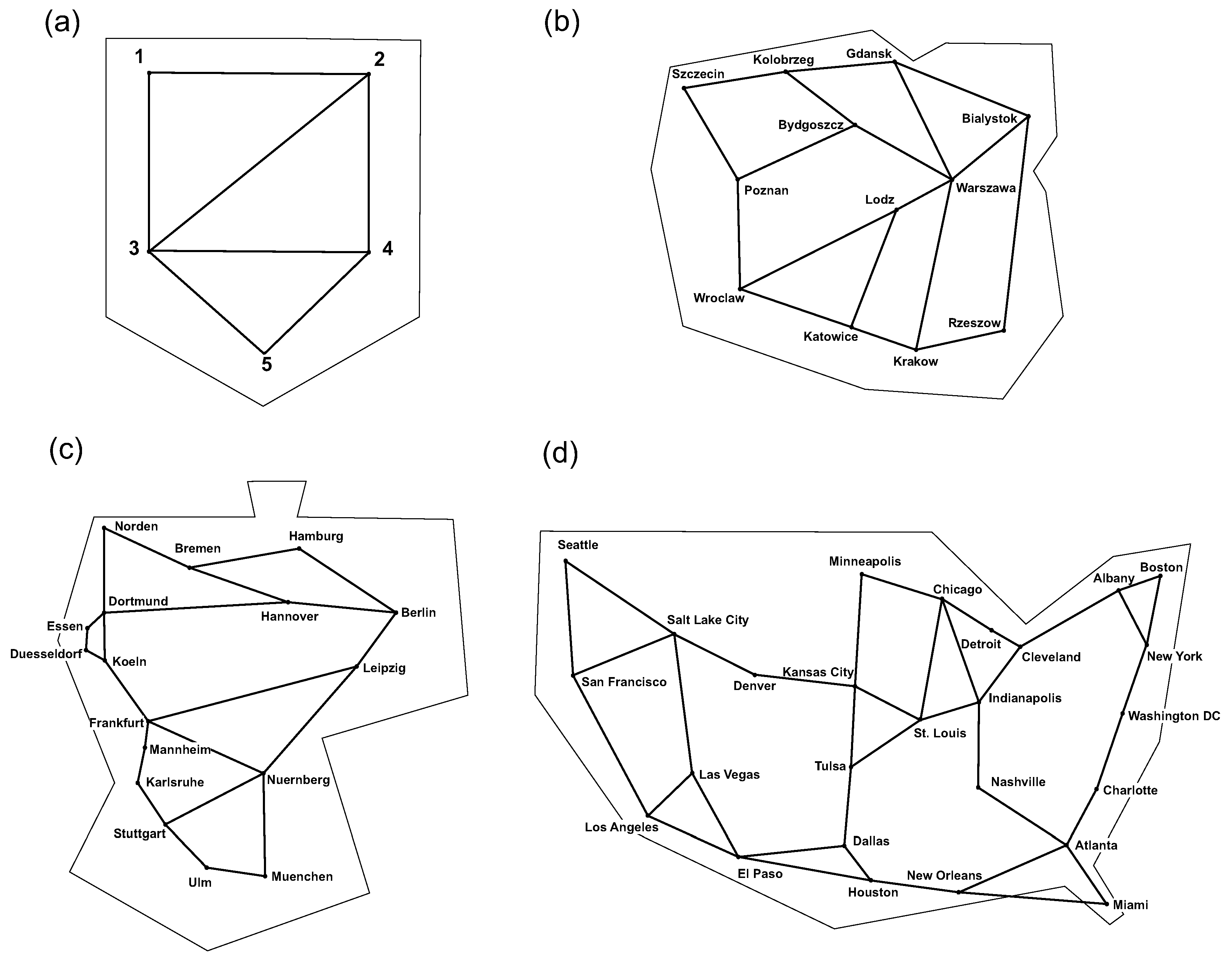
Computational results were obtained for four optical networks with widely varying parameters. The first network was generated artificially and consists of five nodes only while the other networks, i.e., Polish, German and US, correspond to actual optical networks stemming from specified countries and were taken from [17].

Table 1. Analyzed network parameters.

Network	# Nodes	# Link	# Demand
net5	5	14	10
Polish	12	18	66
German	17	26	136
US	26	84	325

and Figure 3 provide the relevant parameters for all four selected networks and their topologies.

Table 2. Node equipment parameters.

Nodal Parameters	T1	T2	T3	M1	M2	WSS
bit rate [Gbps]	10	40	100	-	-	-
number of outputs	1	1	1	-	-	-
cost [cost units]	1	2	5	1	3	3

provides parameters characterizing the nodal equipment. In calculations three types of transponders (T1, T2 and T3) are considered, which vary in offered bit rates and incurred transponder costs. It was assumed that 100 G transponder (T3) is 6 times more expensive than 10 G transponder (T1), and at the same time 3 times more expensive than 40 G transponder (T2). Two types of multiplexers (M1 and M2) are also considered. It is assumed that multiplexers can handle any considered number of wavelengths while they differ in the offered functionality. C-ROADM multiplexer (M1) costs 1 unit while the CDC-ROADM multiplexer (M2) costs 3 cost units. M1 is conventional mux/demux with fixed ports and multiplexer M2 is tunable. Finally, it has been assumed that both C-ROADM and CDC-ROADM use the same wavelength selective switch (WSS), whose price is almost the same as 100 G transponder (T3). Additionally, cost intervention on sites was included and assumed equal 1 unit, in all considered cases.

The demands, which allow for simulation of the traffic intensity, are given by demand matrix, which provides the values of traffic flow between selected nodes expressed in Gbps. An example demand matrix for the network from Figure 3b is presented in

Table 3. An example demands matrix.

Polish	1	2	3	4	5	6	7	8	9	10	11	12
1		7	7	7	7	7	7	7	7	7	7	7
2			7	7	7	7	7	7	7	7	7	7
3				7	7	7	7	7	7	7	7	7
4					7	7	7	7	7	7	7	7
5						7	7	7	7	7	7	7
6							7	7	7	7	7	7
7								7	7	7	7	7
8									7	7	7	7
9										7	7	7
10											7	7
11												7
12

.

The calculations were carried out using a linear solver engine of CPLEX 12.8.0.0 on a 2.1 GHz Xeon E7-4830 v.3 processor with 256 GB RAM running under Linux Debian operating system.

The traffic in an analyzed DWDM network was increased by increasing the demands between initial and end nodes via demand matrix. It was assumed that all entries of the demand matrix were equal, i.e., all elements of the demand matrix were increased simultaneously. The sum of all demand matrix elements that correspond to allocated paths gives an estimate of the network capacity. In the simulations the elements of the demand matrix were increased until integer solution was not feasible. Thus, calculated maximum capacity of DWDM network depends also on the number of wavelengths admitted while searching for the optimum allocation of paths. The number of wavelengths s was set as an input variable and was different for different networks.

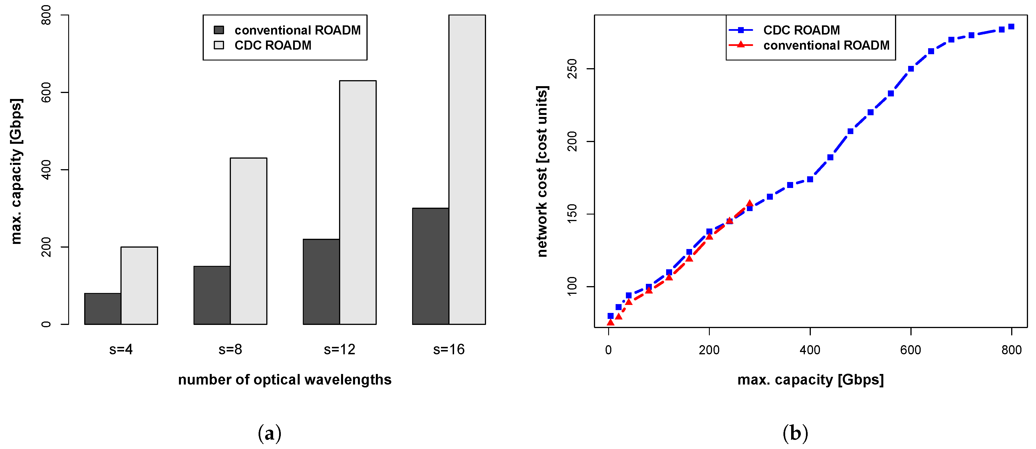
Figure 4, Figure 5, Figure 6 and Figure 7 show the calculated dependence of maximum capacity on the number of DWDM wavelengths and the dependence of network cost on the maximum capacity calculated for the largest number of DWDM wavelengths. For net 5 (Figure 4) results are obtained for 4 different s values equal to 4, 8, 12 and 16. The number of all non-zero elements of the demand matrix (upper triangular part) was 8 while the matrix element values were varied from 5 Gbps to 1 Tbps. Thus, totaling up to maximum network capacity of 8 Tbps. 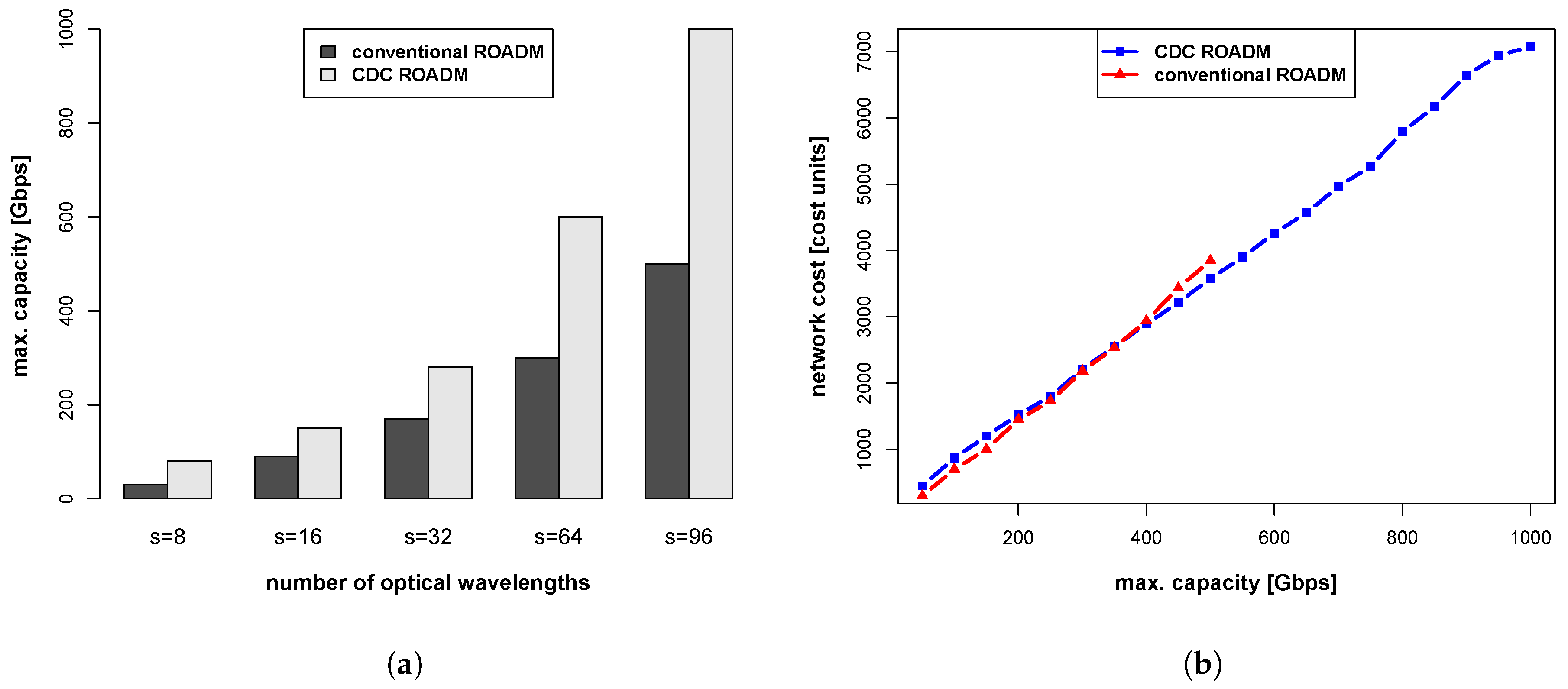For the Polish network (Figure 5) the results are obtained for s values equal to 8, 16, 32, 64 and 96. 66 demands ranging from 5 Gbps to 1 Tbps were considered, totaling up to maximum network capacity of 66 Tbps. 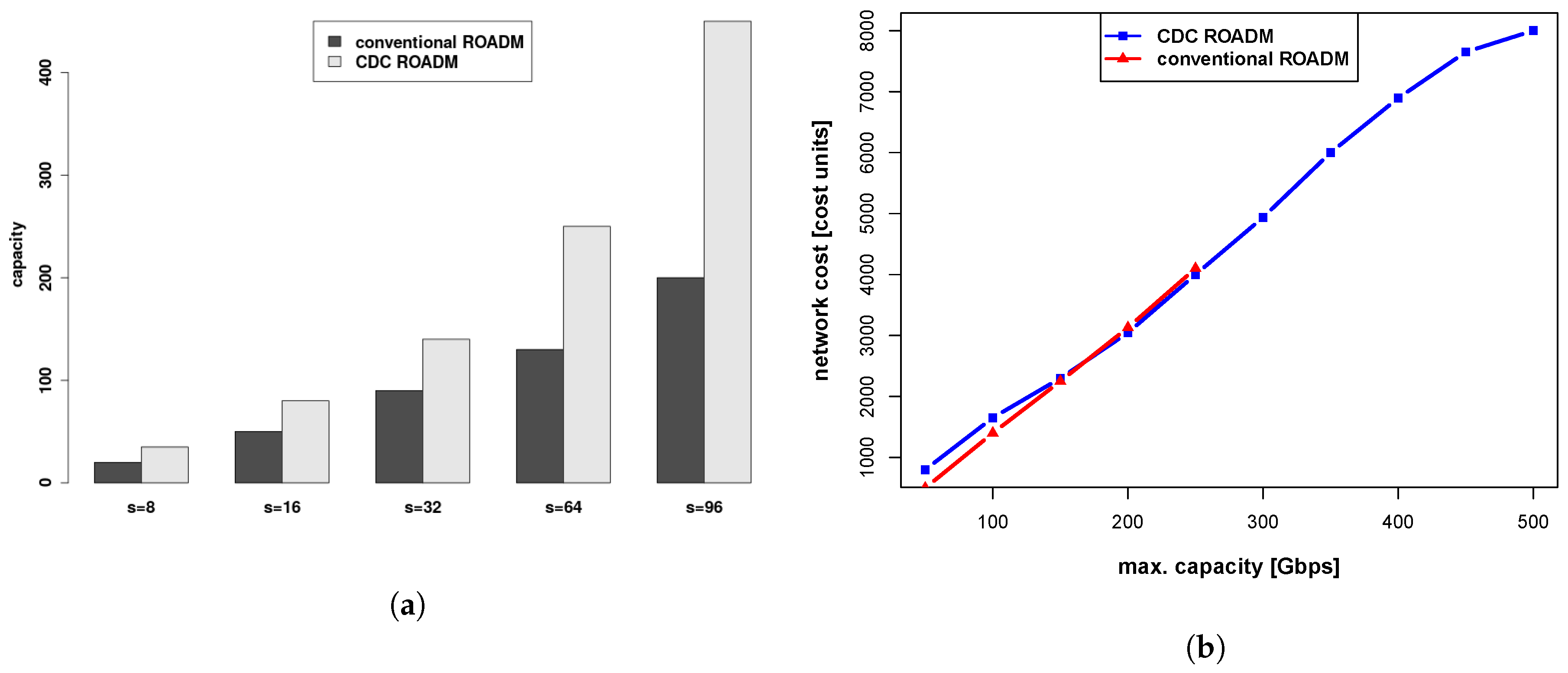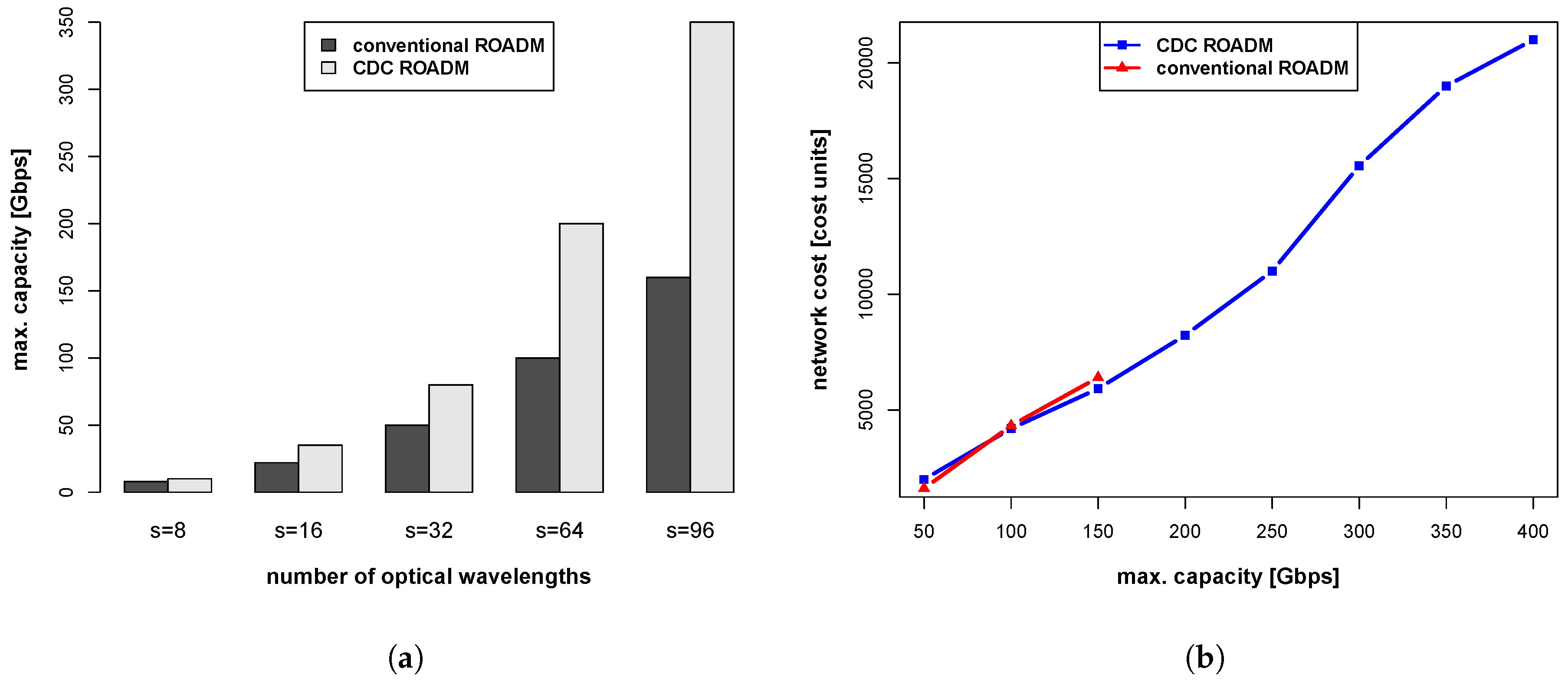In the case of the German network (Figure 6), the results are obtained for s values equal to 8, 16, 32, 64 and 96. 136 demands were varied from 5 Gbps to 500 Gbps, totaling up to maximum network capacity of 68 Tbps. Finally, in the case of the US network (Figure 7) the results are obtained for s values equal to 8, 16, 32, 64 and 96. 325 demands were considered and varied between 5 Gbps and 400 Gbps, totaling up to maximum network capacity of 130 Tbps. The summary of the maximum capacity calculated for each network is shown in

Table 4. Comparison of total network capacity for C-ROADM and CDC-ROADM, for tested networks.

Network	C-ROADM	CDC-ROADM
net5	2.5 Tbps	8 Tbps
Polish	30 Tbps	66 Tbps
German	32 Tbps	68 Tbps
US	43 Tbps	130 Tbps

.

Comparing the results of C-ROADM-based and CDC-ROADM-based networks shown in Figure 4, Figure 5, Figure 6 and Figure 7 shows that the DWDM network using C-ROADM technology becomes congested at much lower values of maximum capacity than the one using CDC-ROADM technology. In fact, CDC-ROADM can handle 2 to 3 times more traffic than C-ROADM-based network. Analyzing the results shown in Figure 4b, Figure 5b, Figure 6b and Figure 7b leads to a conclusion that the costs of allocating demands within DWDM network based on C-ROADM technology are initially lower than in the case of CDC-ROADM technology. However, when C-ROADM-based DWDM network nears to its capacity limit the costs of its further expansion start to grow rapidly and eventually surpass those of CDC-ROADM-based network.

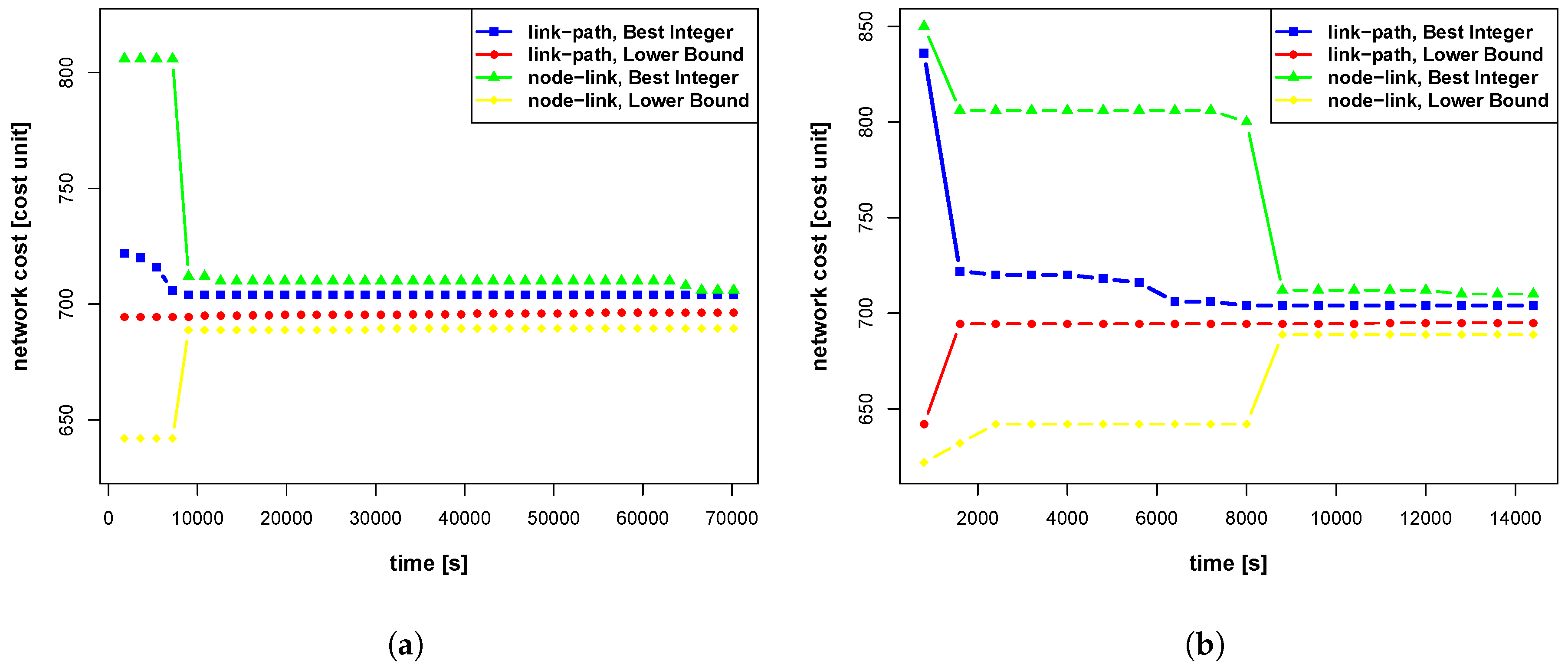
Finally the applicability of integer programming as an optimization tool for considered DWDM networks is validated. In these simulations CPLEX solver execution time was terminated after 20 h (72,000 s) whether the optimal solution was reached or not. If the optimal solution was not found the CPLEX solver returned the best feasible solution and the lower bound.

Table 5. Comparison for Polish network using CDC-ROADM node model of link-path approach (path#) and node-link approach (node-link), while $d=70Gbps$, $s=32$, and $p=1$.

Method	IP Network Cost [Unit Cost]	LP Best Bound	Computation Time [s]	GAP [%]
path1	700	697.5	72,000	0.36
path2	702	696.7	72,000	0.47
path3	702	696.6	72,000	0.77
path4	700	696.3	72,000	0.52
path5	708	696.4	72,000	1.08
path6	704	695.6	72,000	1.19
node-link	706	689.5	72,000	2.34

shows the obtained values of objective function (network cost), computational time and the gap, i.e., the absolute value of the difference between the value of the network cost found using IP and that calculated using LP. The first six cases listed in Table 5 concern the link-path approach, and the last one concerns node-link approach. Nodal parameters were taken from Table 2. The results from Table 5 show that CPLEX solver (IP) did not provide optimal solution but all calculated gaps were small (between 0.36% and 2.34%). Nonetheless, it is noted that the optimal solution was not achieved despite of a long computation time. The nearest to optimal solution was achieved using IP for the case which considers only one path in path-link approach, while the largest gap value was calculated for node-link approach. This is because the node-link approach is characterized by larger space of potential solutions and therefore, a long calculation time is required when using IP, otherwise heuristic methods can be applied to improve the computational efficiency. Figure 8 shows the convergence curves for IP (Best Integer) and LP (Lower Bound) methods for node-link and path-link (path6) approach. These results confirm again that the gap is smaller for the link-path approach than for node-link approach.

4. Conclusions

An optimization of a DWDM network that takes into account details of an optical node has been performed. The study focuses particularly on the comparison of a DWDM network using a C-ROADM with the one applying CDC-ROADM technology while the main objective of the optimization is to minimize optical node resources. A model based on integer programming is proposed, which includes a detailed description of an optical network node architecture. The model is used to study the DWDM network congestion for selected realistic networks with different topologies and traffic demand sets. The results obtained show that CDC-ROADM-based DWDM network is able to carry 2 to 3 times more traffic than a network based on C-ROADM nodes.

A comparison of two approaches, node-link method and link-path method is also presented in the context of the convergence of the algorithm. This comparison shows that link-path approach gives results that are nearer to optimum within a given simulation time. For further improvement of algorithm efficiency both methods should be enhanced by heuristic algorithms.

Finally, it is noted that the results obtained are helpful to telecommunications network operators providing additional guidance while planning a DWDM network expansion.