Dynamic and Stability Analysis of Multibolt Plane Joints under Normal Forces

Abstract

In this paper, a stiffness model of contact surfaces based on a modified three-dimensional fractal contact model is built, which is in accordance with the experiment results. Additionally, the static, dynamic, and stable behaviors of the bolt joint between the spindle box and the machine bed are analyzed. The mathematical relationship between fractal parameters of the surface topography and the stiffness of the system was established to accurately study its static behaviors. Asymmetric curves are observed from the load–deflection results and the nonlinear stiffness characteristic is also presented. It is shown that both the stress and the stiffness increase with the increase of the displacement near the static equilibrium position. Meanwhile, a simplified model without the consideration of roughness is compared with joint interfaces composed from milling, scraping, and grinding surfaces. Numerical calculation was employed to investigate effects of design parameters on the system under harmonic excitation when the processing method, excitation force, bolt pre-tightening force, topography parameters, and other structural parameters, i.e., nominal contact area, joint thickness and bolt number, are eventually regarded as the control parameters. The aim of the article is to analysis the influence of these parameters, including surface morphology, on nonlinear characteristics of the bolt interface with fractal contact surfaces andto provide some references to improve the characteristics.

1. Introduction

The contact interfaces between parts are known as mechanical joint surfaces. These interfaces play an important role in the dynamic behavior of mechanisms and mechanical devices. For example, contact stiffness and damping of such systems at machine tools contribute 60% of the overall stiffness and more than 90% of the overall damping [1,2]. Furthermore, many studies have focused on these joint surfaces. Liu et al. analyzed the dynamic characteristics of the joints in the aero-engine rotor system through FEM simulation and experiment [3]. A virtual gradient material model was proposed by Liao et al. to obtain the contact pressure distribution and dynamic characteristics of the bolted joint [4]. Daouket al. researched the dynamic behavior of the bolted joint under heavy loadings utilizing a bolted structure test bed [5]. Pan et al. built a critical two-degree-of-freedom modal coupling model and studied the effect of contact stiffness on the stability and nonlinearity on the basis of fractal surface topography [6]. Jalaliet al. provided a new linear joint model and investigated the influence of preload and surface roughness quality on the identified equivalent stiffness [7]. A new lump model applied in finite element analysis was given by Beaudoin et al. for the nonlinear dynamic response of bolted flanges [8]. With these interfaces withstanding contact pressures and frictions, the contact problems in engineering include geometry errors, microscopic roughness, lubrication, coating, conduction of heat, and electricity, which are nonlinear and complicated. Therefore, studies of the dynamic characteristics of mechanical joint surfacesare of great significance.

Research on modeling iscrucial for developing simulations to analyze the dynamic motions of contact interfaces. Conventionally, Hertzian contact theory is utilized to model interacting surfaces. As Greenwood and Williamson consider the fact that all engineering surfaces are not absolutely smooth, they describe the contact interfaces with extended Hertzian theory [9]. Rough surfaces are approximated by a series of spherical summits which have the same radius and Gaussian height distributions. The method was first based on statistical representation of the surface topography and is closer to the actual conditions than previous models, and has an enormous influence on contact theory. In the following, many investigations were focused on the extension of G–W model by Bhushan et al. [10], McCool [11], Nayak [12], and Whitehouse et al. [13]. However, Majumdar and Bhushan as well as Sayles and Thomas suggest that statistical roughness parameters depend on both instrumental resolution and sampling length [14,15]. It was found that the Weierstrass–Mandelbrot (W–M) function satisfies all these properties of a surface profile [14,16]. Therefore, fractal theory has been employed to model engineering surfaces by Majumdar and Bhushan (M–B) due to their statistic self-affinity, which is scale-independent [14,17,18,19]. Wang and Komvopoulos introduced the domain extension factor for microcontact size distribution to modify the M–B model [20]. Another fractal-based model was proposed by using a multivariate W–M function [21,22]. According to the previous model, Shuyun Jiang et al. deduced the relationship between stiffness and the real area of contact mathematically [23]. Xiao et al. analyzed the static force–displacement characteristic of joint surfaces on the basis of a two-variable W–M function using the finite element method and further the dynamic behavior of the contact system [22,24].

The above mentioned studies mostly focused on the experiment test or FE method, which is often considered as a macroscopic system. In addition, the previous studies rarely referred to chaos analysis. In this work, the lumped-mass method is applied for the sake of simplicity of computation and the fractal contact model is employed to the perspective of the surface morphology. Based on a single-freedom dynamic model of the bolt joint between the spindle box and the machine bed, which is a typical structure in a machine tool, the influence of design parameters and the load on forced vibration responses has been discussed in order to clarify nonlinear characteristics of the bolt interface. The dynamic model applies to bolted plane joint parts with larger mass. A contact interface regardless of asperities is presented for the purpose of comparison. Moreover, the response analysis can help avoid resonance and chaos by adjusting the parameters in the design process. The outline of this article is as follows. Section 2 outlines a mathematical relationship of the stiffness per unit area and the pressure between joint engineering surfaces, which is verified by the experiment. In Section 3, a single-freedom dynamic model is formulated, where the normal stiffness and damping are treated as functions of fractal parameters. In Section 4, the load–deflection and the stiffness–deflection functions are investigated based onthe kinetic equations obtained. In Section 5, the fourth-order Runge–Kutta method is utilized to study effects of design parameters on the dynamic behaviors and stability of the bolt contact interface. Finally, conclusions are presented concisely in the Section 6.

2. Surface Fractal Contact Model and Verification

The contact interface is an important nonlinearfactor of the bolt joint system. A three-dimensional fractal load–separation contact model modified with the domain extension factor was introduced and the contact stiffness can be obtained byderivationof the curve.

To characterize features of the rough surface topography assuming isotropy, such as continuity, nondifferentiability, and self-affinity, a modified W–M function is given by [23]

$$z\left(x\right)=L{\left(\frac{G}{L}\right)}^{D-1}{\left(\ln \gamma \right)}^{\frac{1}{2}}{\displaystyle \sum _{n=0}^{n_{\max }}{\gamma }^{\left(D-2\right)n}\left[\cos {\phi }_{1n}-\cos \left(\frac{2\pi {\gamma }^{n}x}{L}-{\phi }_{1n}\right)\right]}$$

(1)

where z(x) is the fractal profile, L is the sample length, G is the fractal roughness parameter, D (1 < D < 2) is the fractal dimension, γ (γ >1) is the scaling parameter controls the density of the frequencies in the surface profile, and φ_1n is a random phase. In consideration of surface flatness and frequency distribution density, $\gamma =1.5$ is suitable [21].

The approximate root-mean-square height is obtained as [23]

$$\sigma =\frac{G^{D-1}{L}^{2-D}}{2\sqrt{\left(2-D\right)\ln \gamma }}.$$

(2)

In previous studies, when two flexible bodies with nominally flat surfaces contact with each other, the system is usually replaced by a rigid smooth surface contact with an equivalent elastic rough surface with reduced elastic modulus $E={\left[\left(1-{\nu }_1^2\right)/E_1+\left(1-{\nu }_2^2\right)/E_2\right]}^{-1}$ to make calculation convenient, where E₁, E₂ and ν₁, ν₂ are elastic moduli and Poisson ratios of original surfaces, respectively [23,25]. The stress is derived from the pressure of contact asperities. To simplify the problem, it is normal and reasonable to assume that all asperities have spherical summits with different radiuses [17,21].

For the simple case of elastic–fully plastic material, the normal elastic force p_e at an asperity can be written as [23]

$$p_e\left(a^{\prime }\right)=\frac{2^{\frac{9-2D}{2}}}{3{\pi }^{\frac{3-D}{2}}}{\left(\ln \gamma \right)}^{\frac{1}{2}}{G}^{D-1}E{a^{\prime }}^{\frac{3-D}{2}}$$

(3)

where $a^{\prime }=2a_e$ is the truncated microcontact area belonging to a hypothetical section of the undeformed asperity at the contact position doubles the real microcontact area in elastic deformations and $a^{\prime }=a_p$ in fully plastic deformations.

The critical truncated area $a_c^{\prime }$ is given by [23]

$$a_c^{\prime }={\left[2^{7-2D}{\pi }^{D-1}{b}^{-1}{G}^{2\left(D-1\right)}{\left(\frac{E}{H}\right)}^2\ln \gamma \right]}^{\frac{1}{D-1}}$$

(4)

in which $b={\left(\pi q/2\right)}^2$ and $q=0.454+0.41\nu$, where ν and H are the Poisson ratio and the hardness of the softer material, respectively. It is determined that asperities deform elastically when $a^{\prime }>a_c^{\prime }$.

In addition, the distribution function of the truncated microcontact area is expressed as [20]

$$n\left(a^{\prime }\right)=\frac{D}{2}{\psi }^{\frac{2-D}{2}}{a_l^{\prime }}^{\frac{D}{2}}{a^{\prime }}^{-\frac{D+2}{2}}$$

(5)

where $a_l^{\prime }$ is the largest truncated microcontact area and ψ (ψ > 1) is the domain extension factor. The value of ψ can be obtained by dichotomy method depends on a transcendental equation ${\psi }^{\left(2-D\right)/2}-{\left(1+{\psi }^{-D/2}\right)}^{\left(D-2\right)/D}=\left(2-D\right)/D$.

For light pressure of the interface, asperities are far enough to ignore the effect of their interactions, which leads to a real contact area much smaller than the nominal contact area. A reasonable approximation of the total elastic force P_e can be written as [21]

$$P_e\left(a_l^{\prime }\right)={\displaystyle {\int }_{a_c^{\prime }}^{a_l^{\prime }}{p}_e\left(a^{\prime }\right)}n\left(a^{\prime }\right)d{a}^{\prime }.$$

(6)

Then, substituting Equations (3) and (5) into Equation (6) yields

$$P_e\left(a_l^{\prime }\right)=\{\begin{array}{ll}\frac{2^{\frac{9-2D}{2}}D{G}^{D-1}E{\left(\ln \gamma \right)}^{\frac{1}{2}}{\psi }^{\frac{2-D}{2}}}{3{\pi }^{\frac{3-D}{2}}\left(3-2D\right)}{a_l^{\prime }}^{\frac{D}{2}}\left({a_l^{\prime }}^{\frac{3-2D}{2}}-{a_c^{\prime }}^{\frac{3-2D}{2}}\right),& a_l^{\prime }\ge a_c^{\prime },D\ne \frac{3}{2}\\ 2{\pi }^{-\frac{3}{4}}{G}^{\frac{1}{2}}E{\left(\ln \gamma \right)}^{\frac{1}{2}}{\psi }^{\frac{1}{4}}{a_l^{\prime }}^{\frac{3}{4}}\ln \frac{a_l^{\prime }}{a_c^{\prime }},& a_l^{\prime }\ge a_c^{\prime },D=\frac{3}{2}\\ \\ 0,& a_l^{\prime }<a_c^{\prime }\end{array}.$$

(7)

The truncated contact area is related to $n\left(a^{\prime }\right)$ as follows [21]:

$$A_r^{\prime }\left(a_l^{\prime }\right)={\displaystyle {\int }_0^{a_l^{\prime }}{a}^{\prime }}n\left(a^{\prime }\right)d{a}^{\prime }$$

(8)

Introducing Equation (5) into Equation (8) gives

$$a_l^{\prime }\left(A_r^{\prime }\right)=\frac{2-D}{D}{\psi }^{\frac{D-2}{2}}{A}_r^{\prime }.$$

(9)

If the rough surface obeys the Gaussian distribution, the truncated contact area also can be expressed as a function of the rms height, the separation x_s between the mean planes of the joint interface and the nominal contact area A_a, which is formed as [17]

$$A_r^{\prime }\left(x_s\right)=\frac{A_a}{\sqrt{2\pi }}{\displaystyle {\int }_{\frac{x_s}{\sigma }}^{\infty }{e}^{-\frac{t^2}{2}}dt}=\frac{A_a}{2}\mathrm{erfc}\left(\frac{x_s}{\sqrt{2}\sigma }\right)$$

(10)

where erfc( ) is the complimentary error function and $x_s=x_{s0}-\mathrm{\Delta }{x}_s$, in which x_s0 is the initial separation and Δx_s is the decrease of the distance between the two surfaces.

Hence, the relationship of the separation x_s and the force P_e is obtained mathematically. The normal contact stiffness can be acquired by taking the derivative of P_e with respect to x_s.

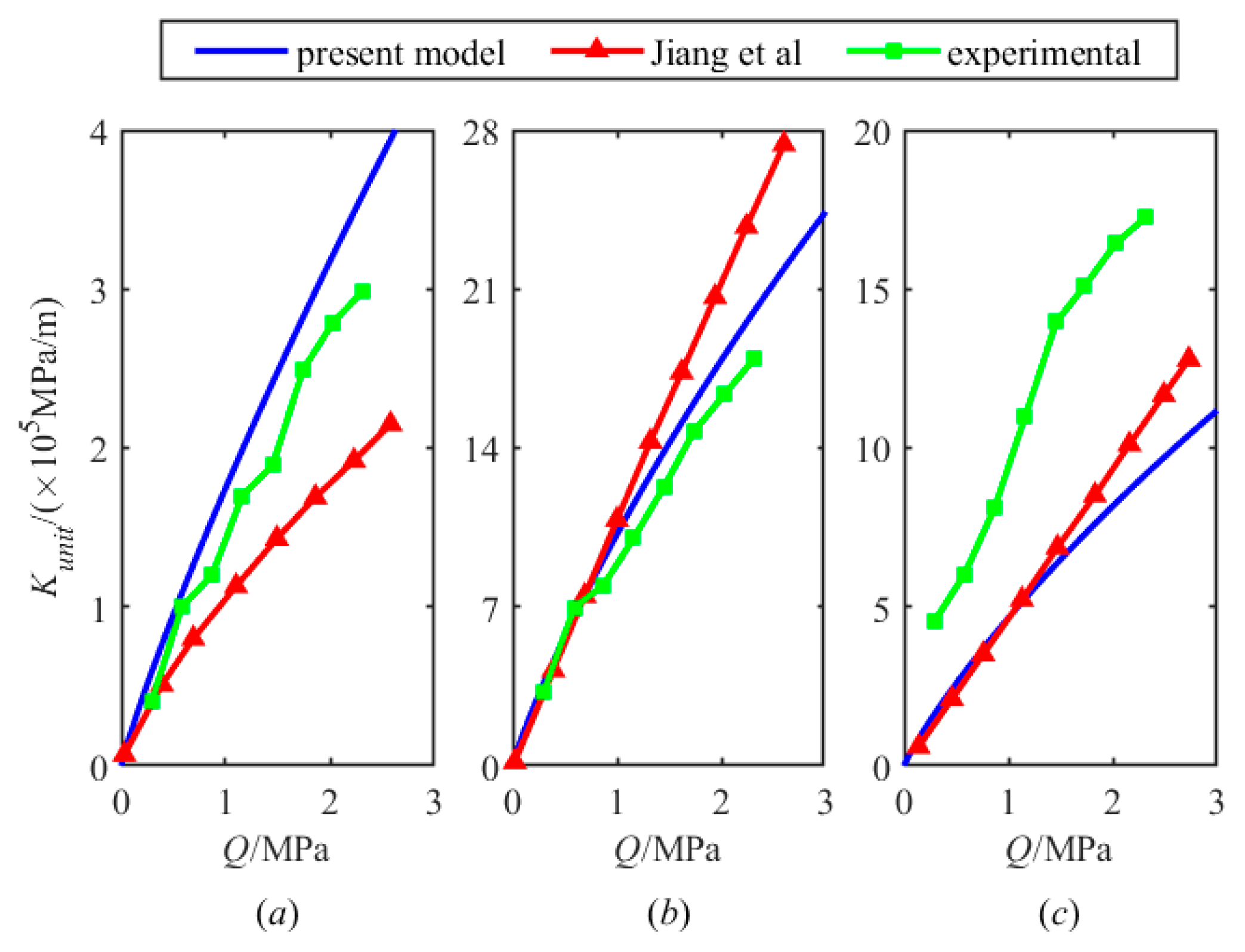
In addition, Jiang et al. have proposed a stiffness model based on the fractal theory and carried out an experimental study utilized cast iron, which is the same as the material of the contact parts in this paper [23]. Figure 1 performs the comparison of numerical simulations of the present model, Jiang’s model, and experiment results of Jiang. It shows the theory curve has good coherence to the experimental data. Here, the pressure of the interface Q and the stiffness per unit area K_unit are obtained as

$$Q\left(a_l^{\prime }\right)=\frac{P_e\left(a_l^{\prime }\right)}{A_a}$$

(11)

$$K_{unit}\left(\mathrm{\Delta }{x}_s\right)=\frac{K_s\left(\mathrm{\Delta }{x}_s\right)}{A_a}$$

(12)

where the stiffness of contact surfaces $K_s\left(\mathrm{\Delta }{x}_s\right)=d{P}_e\left(\mathrm{\Delta }{x}_s\right)/d\mathrm{\Delta }{x}_s$.

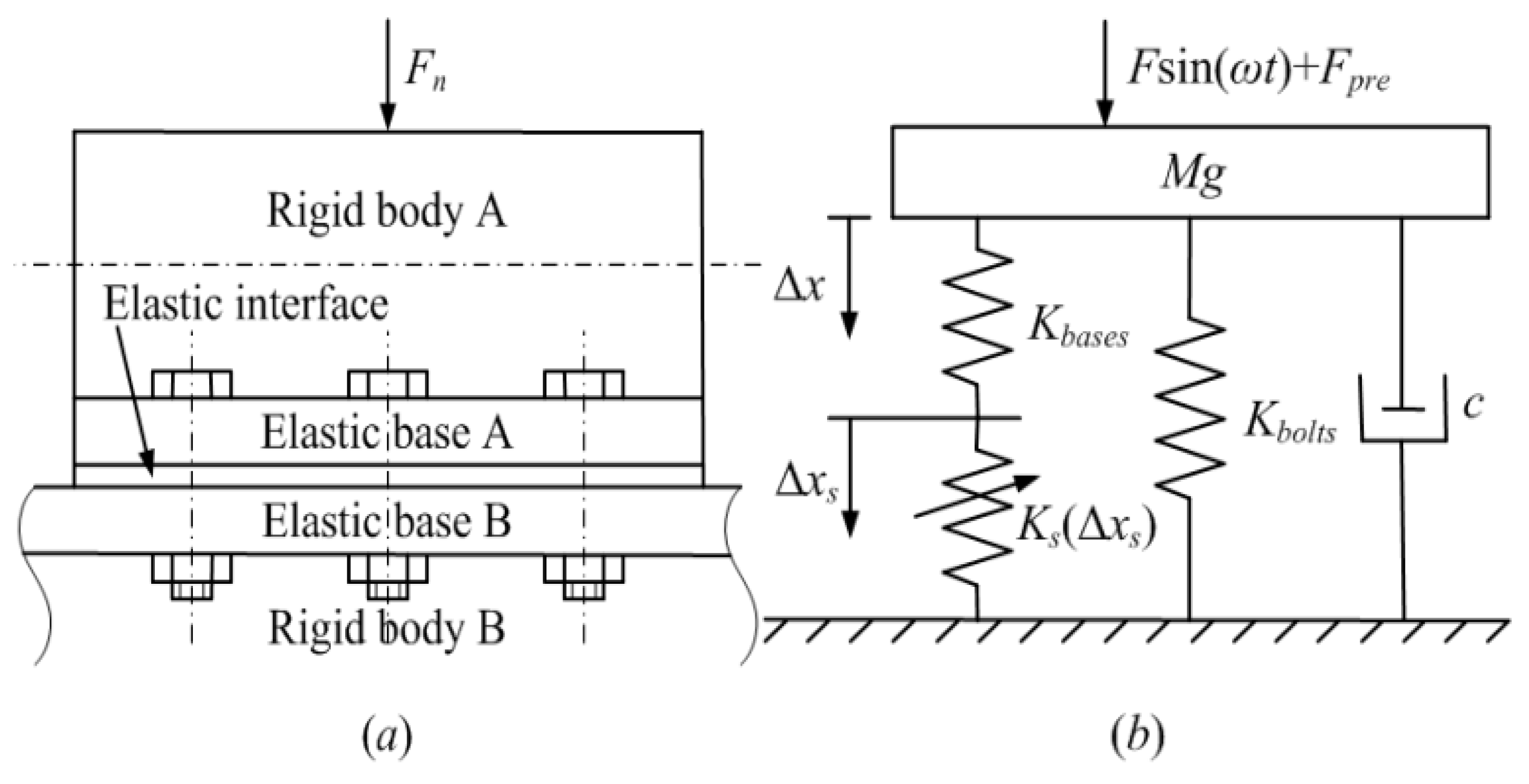
3. Dynamic Model of the Bolt Joint Interface

In this section, a model of the spindle box in contact with the machine bed is built to analyze the dynamic characteristic of the fixed joint parts. For simplicity, contact objects are considered to be a series of asperities according to the equivalent surface on base B, two elastic smooth bases A (with a rigid bottom plane), B connected by bolts and two rigid bodies A, B, which is performed in Figure 2a. It has been assumed that pressures on bases are evenly distributed. The stiffness of serial bulks is defined as $K_{bases}=K_1+K_2$, in which $K_1={E_1{A}_a/l}_1$ and $K_2={E_2{A}_a/l}_2$, where l₁ and l₂ are the thickness of bulks respectively. Deformation occurs at those asperities leading to a contact stiffness K_s. The total stiffness of bolts $K_{bolts}=m{k}_{bolt}$ is determined by the type and number m. As demonstrated in Figure 2a, K_s and K_bases are in series, and in parallel with K_bolts. On the basis of the structure, a single-degree-of-freedom model of the system is established in Figure 2b. The parameter c is the damping coefficient of the system. The distance variation Δx between the most remote two surfaces belong to bases and the variation Δx_s are caused by a harmonic excitation Fsin(ωt) in this model. Initial distances, $x_{pre}=x+\mathrm{\Delta }x$ and $x_{spre}=x_s+\mathrm{\Delta }{x}_s$, corresponding to these two variables are both due to the mass of the spindle box M and the pretension force of bolts $F_{pre}=m{f}_{pre}$, where the subscript pre denotes the system is static equilibrium and preloaded by bolts.

In order to obtain the force between the interfaceundervibration condition, aphenomenon is introducedthat even though the large plastic deformation occurs during the load process, the unloading process is completely elastic [26]. Therefore, the stressbetweencontact surfaces of a mechanical joint under repeated loading can beconsidered as an elastic force only, which is acquired by Equation (7). The kinetic equation is given by

$$\{\begin{array}{ll}M\mathrm{\Delta }\ddot{x}+c\mathrm{\Delta }\dot{x}+K_{bolts}\mathrm{\Delta }x+P_e\left(x_{spre}-\mathrm{\Delta }{x}_s\right)=Mg+F_{pre}+F\sin \left(\omega t\right),& \mathrm{\Delta }x\le \mathrm{\Delta }{x}_{bpre}\\ M\mathrm{\Delta }\ddot{x}+c\mathrm{\Delta }\dot{x}+P_e\left(x_{spre}-\mathrm{\Delta }{x}_s\right)=Mg+F\sin \left(\omega t\right),& \mathrm{\Delta }x>\mathrm{\Delta }{x}_{bpre}\end{array}$$

(13)

in which x_spre satisfied the function $P_e\left(x_{spre}\right)=Mg+F_{pre}$, and $\mathrm{\Delta }{x}_{bpre}=f_{pre}/k_{bolt}$ is the elongation of preloaded bolts.

Moreover, $P_e\left(x_{spre}-\mathrm{\Delta }{x}_s\right)-P_e\left(x_{spre}\right)=K_{bases}\left(\mathrm{\Delta }x-\mathrm{\Delta }{x}_s\right)$ is known according to Figure 2b to deduce the function $\mathrm{\Delta }x=f\left(\mathrm{\Delta }{x}_s\right)=\left[P_e\left(x_{spre}-\mathrm{\Delta }{x}_s\right)-P_e\left(x_{spre}\right)\right]/K_{bases}+\mathrm{\Delta }{x}_s$. Substituting this relationship into Equation (13) yields

$$\{\begin{array}{ll}M\mathrm{\Delta }\ddot{x}+c\mathrm{\Delta }\dot{x}+\left(K_{bases}+K_{bolts}\right)\mathrm{\Delta }x-K_{bases}{f}^{-1}\left(\mathrm{\Delta }x\right)=F\sin \left(\omega t\right),& \mathrm{\Delta }x\le \mathrm{\Delta }{x}_{bpre}\\ M\mathrm{\Delta }\ddot{x}+c\mathrm{\Delta }\dot{x}+K_{bases}\mathrm{\Delta }x-K_{bases}{f}^{-1}\left(\mathrm{\Delta }x\right)=F\sin \left(\omega t\right)-F_{pre},& \mathrm{\Delta }x>\mathrm{\Delta }{x}_{bpre}\end{array}.$$

(14)

Introducing the overall stiffness at static balance $K_{npre}=K_{bases}{K}_{spre}/\left(K_{bases}+K_{spre}\right)+K_{bolts}$, where $K_{spre}=K_s\left(0\right)$ depends on the value of $x_{s0}=x_{spre}$, the dimensionless equation of the vertical vibration model can be obtained by defining $\tau =\omega t$, ${\omega }_n=\sqrt{K_{npre}/M}$, $\overline{\omega }=\omega /{\omega }_n$, $\zeta =c/\left(2M{\omega }_n\right)$, $\overline{F}=F/K_{npre}$, ${\overline{F}}_{pre}=F_{pre}/K_{npre}$, ${\overline{K}}_{bases}=K_{bases}/K_{npre}$, ${\overline{K}}_{bolts}=K_{bolts}/K_{npre}$, and $\overline{f}\left(\mathrm{\Delta }{x}_s\right)=\left[{\overline{P}}_e\left(x_{spre}-\mathrm{\Delta }{x}_s\right)-{\overline{P}}_e\left(x_{spre}\right)\right]/{\overline{K}}_{bases}+\mathrm{\Delta }{x}_s=f\left(\mathrm{\Delta }{x}_s\right)$, in which ${\overline{P}}_e=P_e/K_{npre}$.

The equation of motion is transformed into the dimensionless form

$${\overline{\omega }}^2\frac{d^2\mathrm{\Delta }x}{d{\tau }^2}+2\zeta \overline{\omega }\frac{d\mathrm{\Delta }x}{d\tau }+\overline{g}\left(\mathrm{\Delta }x\right)=\overline{F}\sin \tau$$

(15)

where $\zeta =0.005$ [27] and $\overline{g}\left(\mathrm{\Delta }x\right)=\{\begin{array}{ll}\left({\overline{K}}_{bases}+{\overline{K}}_{bolts}\right)\mathrm{\Delta }x-{\overline{K}}_{bases}{\overline{f}}^{-1}\left(\mathrm{\Delta }x\right),& \mathrm{\Delta }x\le \mathrm{\Delta }{x}_{bpre}\\ {\overline{K}}_{bases}\mathrm{\Delta }x-{\overline{K}}_{bases}{\overline{f}}^{-1}\left(\mathrm{\Delta }x\right)+{\overline{F}}_{pre},& \mathrm{\Delta }x>\mathrm{\Delta }{x}_{bpre}\end{array}$.

By contrast, if the roughness of contact surfaces is neglected, the dynamic model changes into an ideal model and Δx_s can be expressed in the form

$$\mathrm{\Delta }{x}_s=\{\begin{array}{ll}\mathrm{\Delta }x-\mathrm{\Delta }{x}_{apre},& \mathrm{\Delta }x\le \mathrm{\Delta }{x}_{apre}\\ 0,& \mathrm{\Delta }x>\mathrm{\Delta }{x}_{apre}\end{array}$$

(16)

in which $\mathrm{\Delta }{x}_{apre}=-\frac{Mg+F_{pre}}{K_{bases}}$.

Equation (14) can be transformed into

$$\{\begin{array}{ll}M\mathrm{\Delta }\ddot{x}+c\mathrm{\Delta }\dot{x}+K_{bolts}\mathrm{\Delta }x=F\sin \left(\omega t\right)+Mg+F_{pre},& \mathrm{\Delta }x\le \mathrm{\Delta }{x}_{apre}\\ M\mathrm{\Delta }\ddot{x}+c\mathrm{\Delta }\dot{x}+\left(K_{bases}+K_{bolts}\right)\mathrm{\Delta }x=F\sin \left(\omega t\right),& \mathrm{\Delta }{x}_{apre}<\mathrm{\Delta }x\le \mathrm{\Delta }{x}_{bpre}\\ M\mathrm{\Delta }\ddot{x}+c\mathrm{\Delta }\dot{x}+K_{bases}\mathrm{\Delta }x=F\sin \left(\omega t\right)-F_{pre},& \mathrm{\Delta }x>\mathrm{\Delta }{x}_{bpre}\end{array}.$$

(17)

As $\mathrm{\Delta }{x}_s=0$ in a small neighborhood of $\mathrm{\Delta }x=0$, the contact stiffness at the static equilibrium position K_spre is infinite, and then $K_{npre}=K_{bases}+K_{bolts}$ is achieved. Introducing the parameter $\overline{G}=Mg/K_{npre}$, the dimensionless equation is as follows

$${\overline{\omega }}^2\frac{d^2\mathrm{\Delta }x}{d{\tau }^2}+2\zeta \overline{\omega }\frac{d\mathrm{\Delta }x}{d\tau }+\overline{h}\left(\mathrm{\Delta }x\right)=\overline{F}\sin \tau$$

(18)

where $\overline{h}\left(\mathrm{\Delta }x\right)=\{\begin{array}{ll}{\overline{K}}_{bolts}\mathrm{\Delta }x-\overline{G}-{\overline{F}}_{pre},& \mathrm{\Delta }x\le \mathrm{\Delta }{x}_{apre}\\ \left({\overline{K}}_{bases}+{\overline{K}}_{bolts}\right)\mathrm{\Delta }x,& \mathrm{\Delta }{x}_{apre}<\mathrm{\Delta }x\le \mathrm{\Delta }{x}_{bpre}\\ {\overline{K}}_{bases}\mathrm{\Delta }x+{\overline{F}}_{pre},& \mathrm{\Delta }x>\mathrm{\Delta }{x}_{bpre}\end{array}$.

The force between bases is obtained as

$$\overline{P}\left(\mathrm{\Delta }x\right)=\{\begin{array}{ll}0,& \mathrm{\Delta }x\le \mathrm{\Delta }{x}_{apre}\\ {\overline{K}}_{bases}\mathrm{\Delta }x+\overline{G}+{\overline{F}}_{pre},& \mathrm{\Delta }x>\mathrm{\Delta }{x}_{apre}\end{array}.$$

(19)

4. Force–Displacement Characteristic of the Bolt Joint Interface

To analyze the dynamic performance of the system, the stiffness should be obtained. On the basis of Equation (14) in Section 3, kinetic equation without inertia force and damping force illustrates the relationship between the normal external load F_n and Δx under slow load rate, which is given by

$$F_n\left(\mathrm{\Delta }x\right)=\{\begin{array}{ll}\left(K_{bases}+K_{bolts}\right)\mathrm{\Delta }x-K_{bases}{f}^{-1}\left(\mathrm{\Delta }x\right),& \mathrm{\Delta }x\le \mathrm{\Delta }{x}_{bpre}\\ K_{bases}\mathrm{\Delta }x-K_{bases}{f}^{-1}\left(\mathrm{\Delta }x\right)+F_{pre},& \mathrm{\Delta }x>\mathrm{\Delta }{x}_{bpre}\end{array}.$$

(20)

Furthermore, with the ignorance of unevenness, Equation (17) can be simplified as

$$F_n\left(\mathrm{\Delta }x\right)=\{\begin{array}{ll}{K}_{bolts}\mathrm{\Delta }x-Mg-F_{pre},& \mathrm{\Delta }x\le \mathrm{\Delta }{x}_{apre}\\ \left(K_{bases}+K_{bolts}\right)\mathrm{\Delta }x,& \mathrm{\Delta }{x}_{apre}<\mathrm{\Delta }x\le \mathrm{\Delta }{x}_{bpre}\\ K_{bases}\mathrm{\Delta }x+F_{pre},& \mathrm{\Delta }x>\mathrm{\Delta }{x}_{bpre}\end{array}.$$

(21)

Taking the derivative of F_n with respect to Δx, the total stiffness K_n is written as

$$K_n\left(\mathrm{\Delta }x\right)=\{\begin{array}{ll}\frac{K_{bases}{K}_s\left[f^{-1}\left(\mathrm{\Delta }x\right)\right]}{K_{bases}+K_s\left[f^{-1}\left(\mathrm{\Delta }x\right)\right]}+K_{bolts},& \mathrm{\Delta }x\le \mathrm{\Delta }{x}_{bpre}\\ \frac{K_{bases}{K}_s\left[f^{-1}\left(\mathrm{\Delta }x\right)\right]}{K_{bases}+K_s\left[f^{-1}\left(\mathrm{\Delta }x\right)\right]},& \mathrm{\Delta }x>\mathrm{\Delta }{x}_{bpre}\end{array}.$$

(22)

When roughnesses are overlooked, the expression of K_n is transformed into

$$K_n\left(\mathrm{\Delta }x\right)=\{\begin{array}{ll}{K}_{bolts},& \mathrm{\Delta }x\le \mathrm{\Delta }{x}_{apre}\\ K_{bases}+K_{bolts},& \mathrm{\Delta }{x}_{apre}<\mathrm{\Delta }x\le \mathrm{\Delta }{x}_{bpre}\\ K_{bases},& \mathrm{\Delta }x>\mathrm{\Delta }{x}_{bpre}\end{array}.$$

(23)

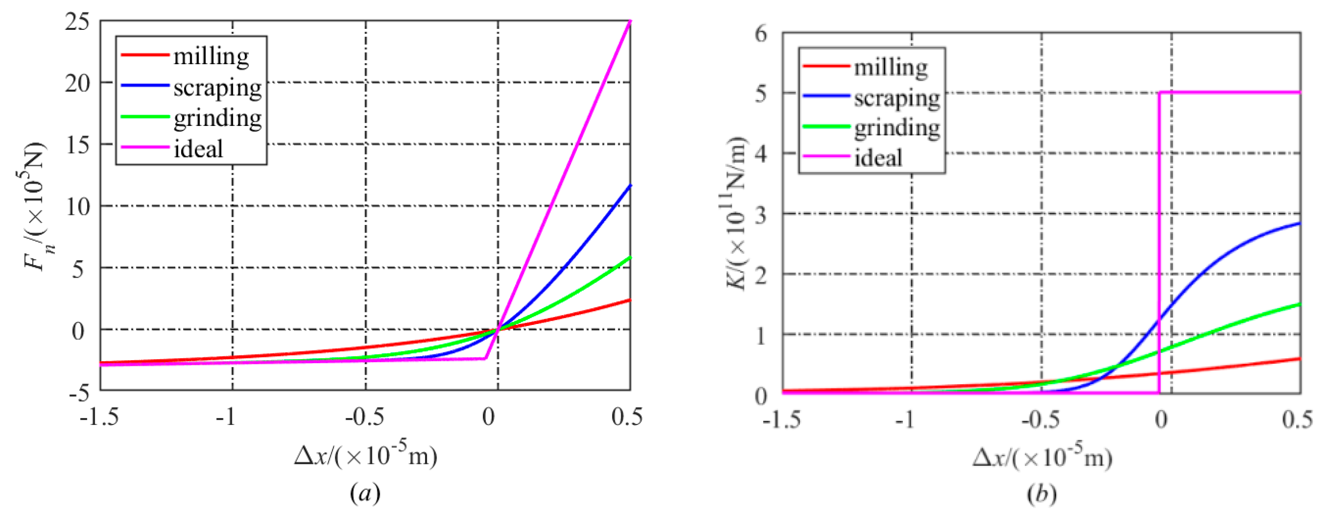
The influence of different manufacturing methods on the static behavior of the system is shown in Figure 3. As demonstrated in Figure 3a, the slope of curves increases except for that of ideal surfaces, indicating a hardening nonlinear behavior when Δx > 0 and a softening nonlinear behavior when Δx < 0. This phenomenon is more apparently for scraping/scraping joint which has a smoother equivalent surface in −0.5 × 10⁻⁵ m < Δx < 0.5 × 10⁻⁵ m. With the decrease of the displacement in the negative direction, these curves are closer to each other. It is caused by the interface separation of the contact pairs. Figure 3b shows that the stiffness without the consideration of asperities is piecewise-linear over the whole displacement range and greater than others when Δx > 0. All the curves intersect each other, and the crossing points are observed in −0.5 × 10⁻⁵ m < Δx < 0. The parameters of bolt joint surfaces are shown in

Table 1. Partial parameters of the system.

E1, E2 (GPa)	ν1, ν2	l1, l2 (mm)	H (HB)	M (kg)	Aa (mm2)	m	fpre (kN)	kbolt (N/m)	Kbases (N/m)
100	0.25	15	220	300	1.491 × 105	6	38.4	5.7865 × 108	4.9692 × 1011

and

Table 2. Partial parameters of the system.

Manufacturing Method	Ra (μm)	L (mm)	Deqa	Geqa (m)
milling	3.49	4	1.2183	5.9036 × 10−14
scraping	1.20		1.7674	1.1850 × 10−7
grinding	1.44		1.4058	2.2826 × 10−10

Values of topography parameters are the experiment data in the study by Jiang et al., ^a subscript eq denotes that D_eq and G_eq are equivalent fractal parameters.

[23].

5. Results

This section is concerned with effects of the dimensionless parameter, excitation force $\overline{F}$, and design parameters, i.e., processing method, equivalent fractal dimension D_eq, equivalent fractal roughness G_eq, nominal contact area A_a, thickness of the joint l = l₁ + l₂, bolt number m and bolt pre-tightening f_pre of the system on the dynamic behaviors and stability in excitation frequency $\overline{\omega }$ utilizing the fractal parameters of the milling/milling joint in Table 2. The fourth-order Runge–Kutta method was employed to calculate the numerical solutions. Equations (7), (9), (10), and (13) indicate that nine parameters are independent for the present system, which are M, c, K_bolts, D_eq, G_eq, A_a, F, ω, and Δx_bpre. Thus, ω and F are converted into proper dimensionless indexes $\overline{\omega }$ and $\overline{F}$. Parameters c, K_bolts, and Δx_bpre have exhibited some correlations existed with ζ, M, D_eq, G_eq, A_a, l, m, and f_pre, respectively, in previous analysis, where ζ and M are assumed to remain constant values. All the parameters of the joint interface are still provided by Table 1.

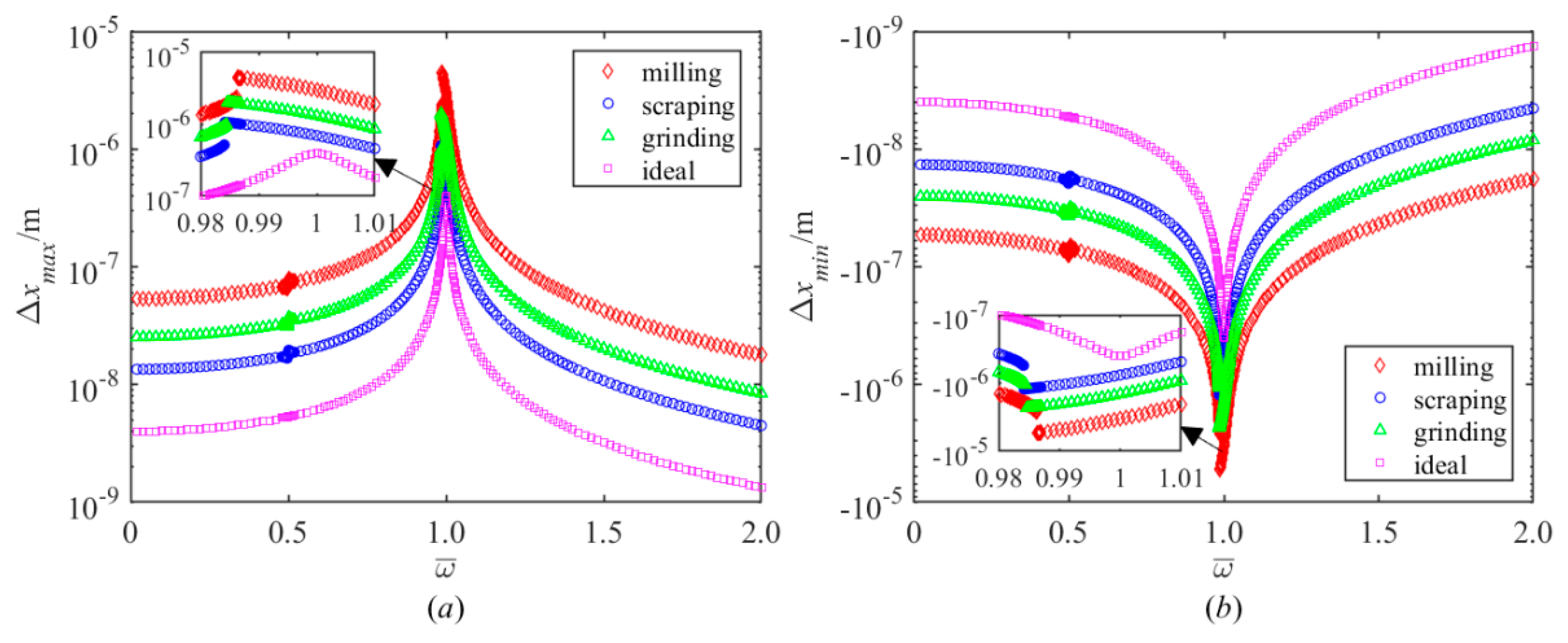
5.1. Effect of Manufacturing Methodon Nonlinear Response

In general, the surface appearance changes the dynamic behavior of the joint interface. The distinction among milling, scraping, grinding, and smooth surfaces was studied. For the amplitude of excitation, force F is fixed as 2000 N, and results of numerical simulations are demonstrated in Figure 4, whichexhibits softening type nonlinearity, and there appears to be a jumping phenomenon except for smooth surfaces. With the roughness R_a of the machined surface increases, the primary resonance frequency and the maximum amplitude of the system increase. It is also found the system has a tendency of occurrence of superharmonic resonance near $\overline{\omega }=0.5$.

5.2. Effect of Excitation Force on Nonlinear Response

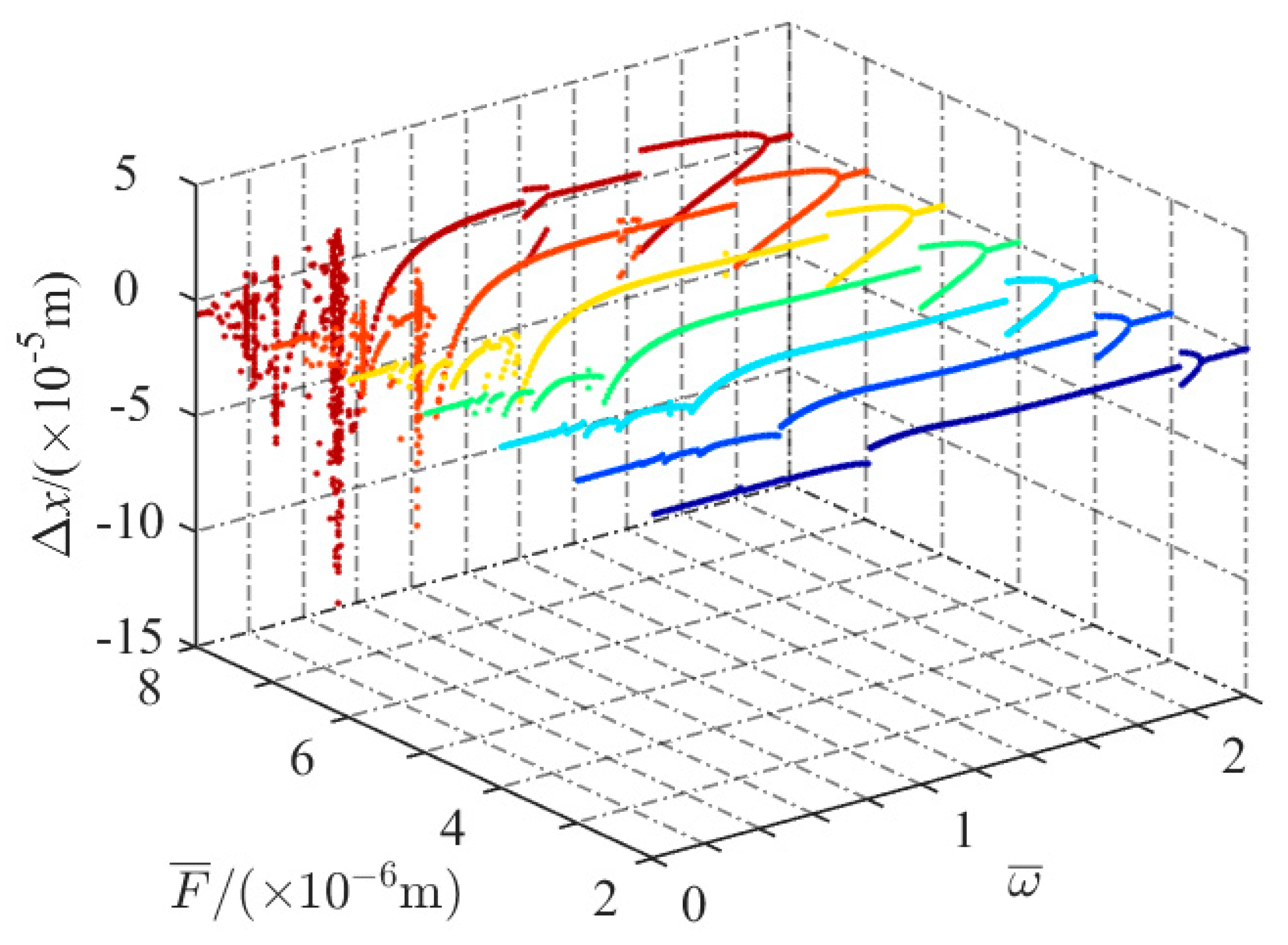
In this subsection, the gradual change between period motion and chaotic motion in different dimensionless excitation forces $\overline{F}$ are shown in Figure 5. It is observed that a 2T-period response occurs from frequency ratio $\overline{\omega }=1.96$ to $\overline{\omega }=2.03$ for $\overline{F}=2\times {10}^{-6}\mathrm{m}$. With the increase of $\overline{F}$, another region of 2T-period motion near $\overline{\omega }=0.63$ and region of 3T-period motion near $\overline{\omega }=1.4$ appear in succession when $\overline{F}=4\times {10}^{-6}\mathrm{m}$ and $\overline{F}=6\times {10}^{-6}\mathrm{m}$, respectively. As $\overline{F}$ is further increased, chaotic behavior is visible gradually at several points before $\overline{\omega }=0.6$. In the meantime, 2T- and 3T-period motion regions and chaos regions are enlarged, and the midpoints of these regions move towards the negative direction.

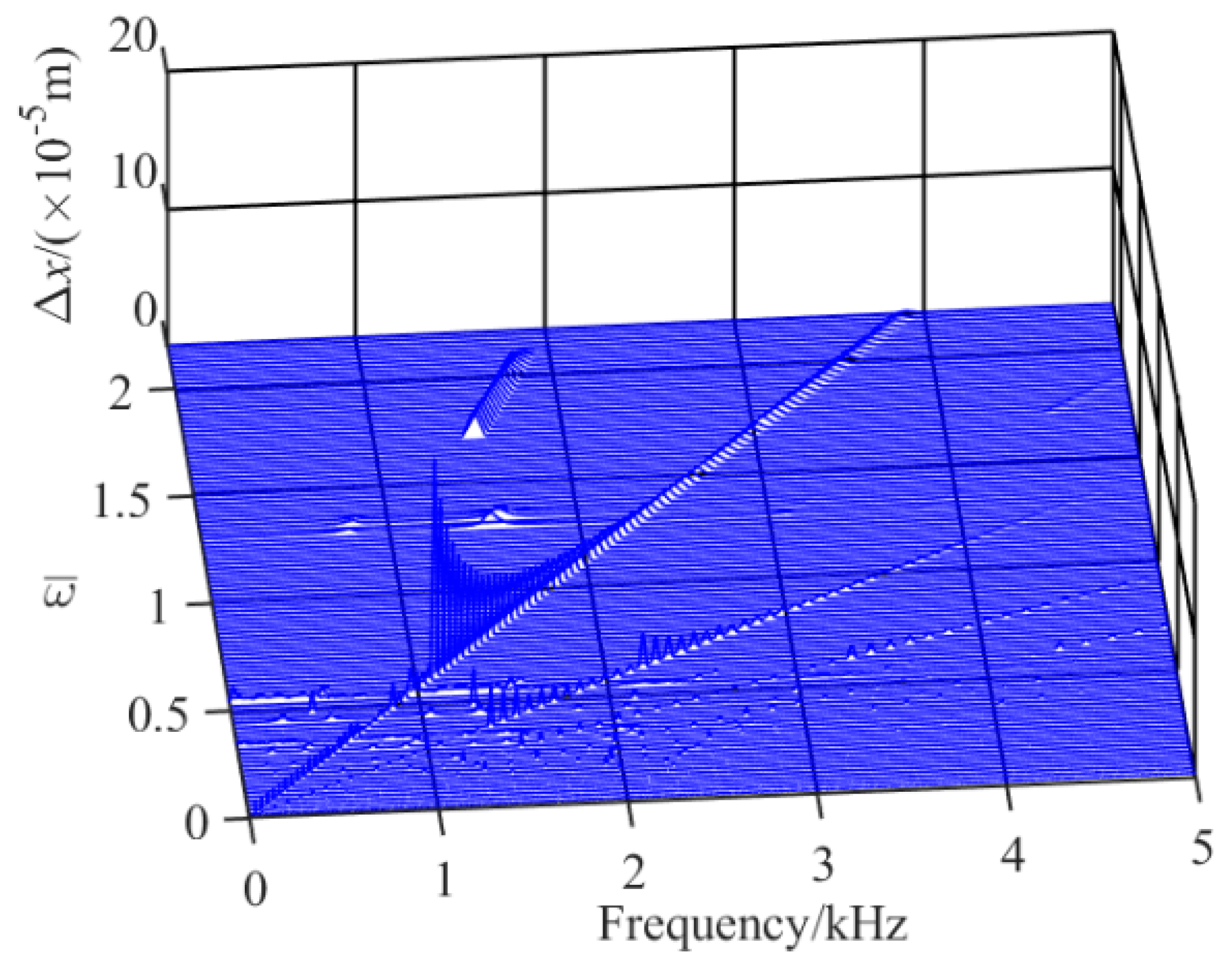
For $\overline{F}=7\times {10}^{-6}\mathrm{m}$, a 3-D waterfall chart with the frequency ratio as control parameter is illustrated in Figure 6. With the increase of $\overline{\omega }$, there appears a jumping phenomenon in the excitation frequency component at $\overline{\omega }=0.61$. It can also be seen that super- and subharmonic vibrations occur in different regions. The system generates a subharmonic, which leads to the bifurcation phenomenon. When the frequency spectrum is continuous near $\overline{\omega }=0.34$ and $\overline{\omega }=0.54$, the system performs chaotic motion, which is according with data in Figure 5.

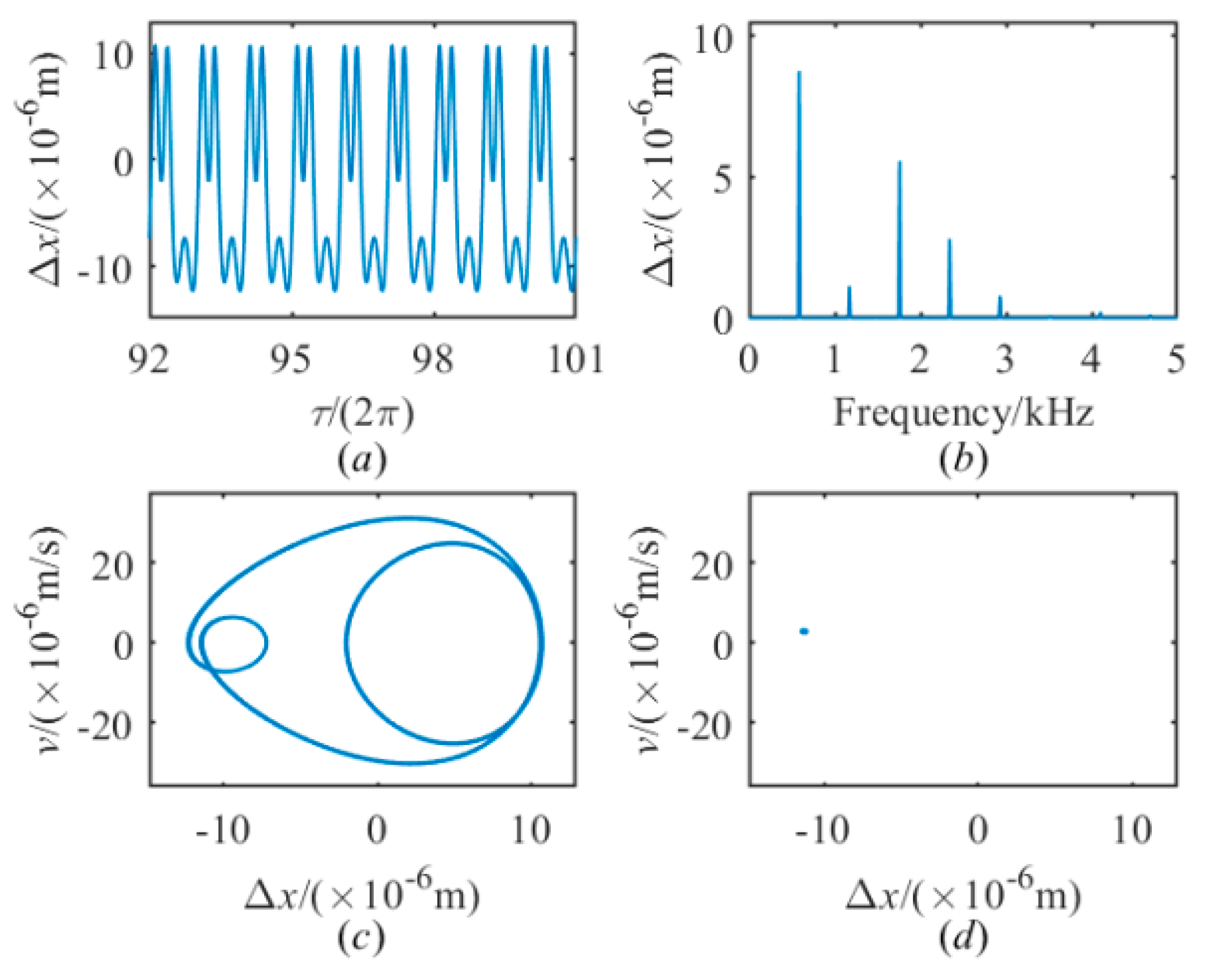
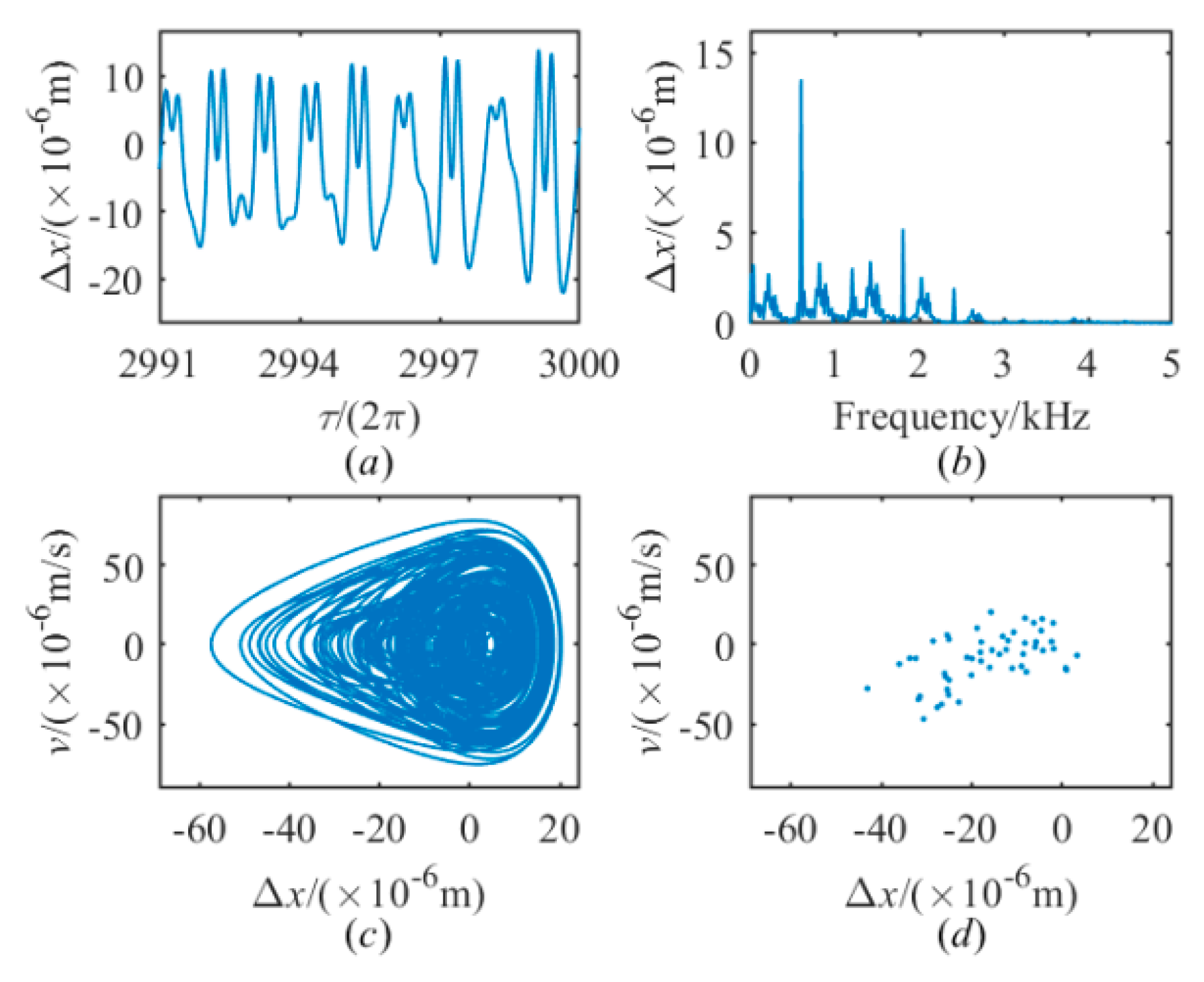
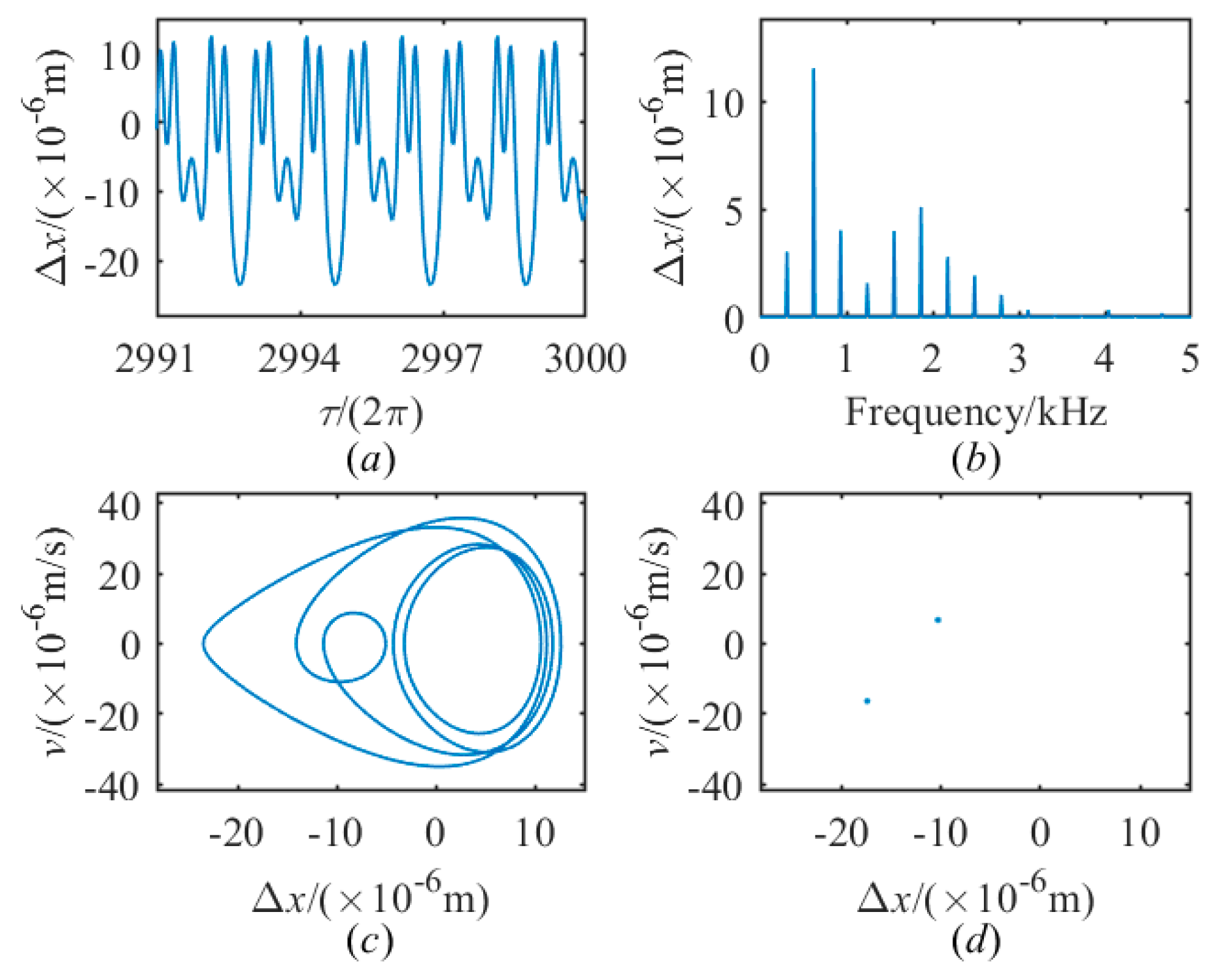
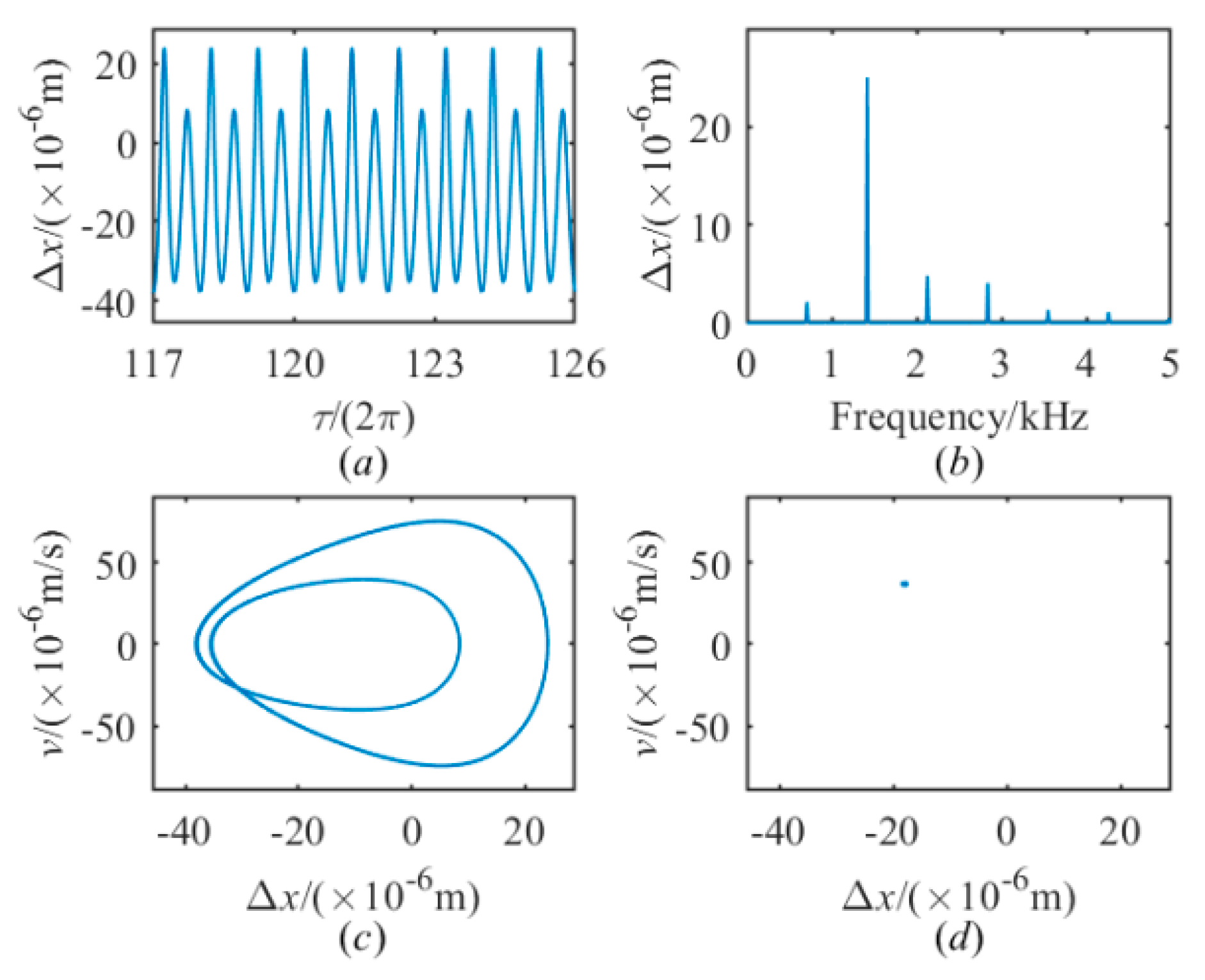
To explain more clearly, Figure 7, Figure 8, Figure 9 and Figure 10 demonstrate the time histories, frequency spectrums, phase plane diagrams, and Poincare sections under four different excitation frequencies for $\overline{F}=7\times {10}^{-6}\mathrm{m}$. In Figure 7, the joint interface shows a 1T-period motion at $\overline{\omega }=0.33$. However, as $\overline{\omega }$ is increased to 0.34, the 1T-period motion is replaced by chaotic motion, which is seen in Figure 8. When $\overline{\omega }$ reaches 0.35, the system transits from chaotic motion to 2T-period motion is shown in Figure 9. Since the frequency spectrum is continuous and a number of discrete points appear in the Poincare section, chaotic behavior is obviously visible. At $\overline{\omega }=0.4$, the motion transits from 2T-period motion back to 1T-period motion is exhibited in Figure 10. From Figure 7, Figure 8, Figure 9 and Figure 10, it can be observed that superharmonics exist in each frequency spectrum.

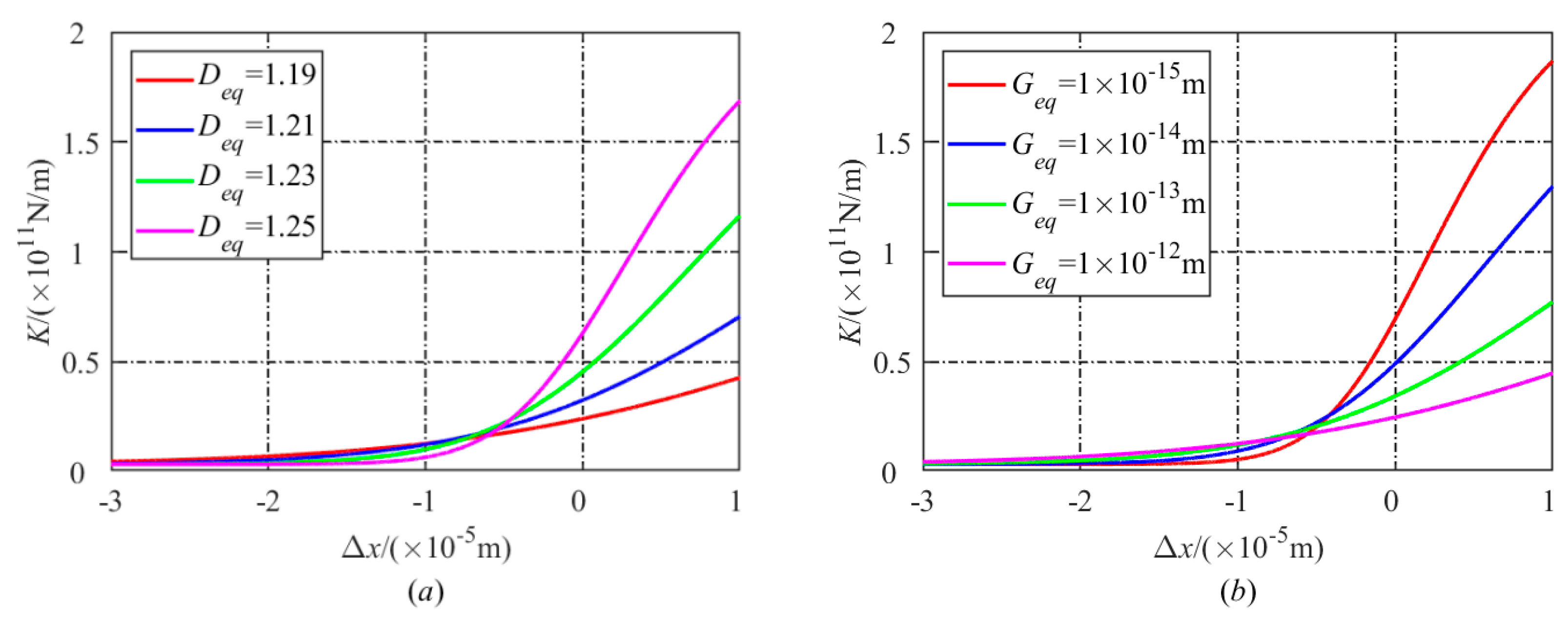
5.3. Effect of Fractal Parameters of Surface Topography

According to Equation (1), the surface topography is determined from the fractal dimension D and the fractal roughness G. Figure 11 shows that the stiffness with respect to the displacement in different equivalent fractal parameters. All the curves are monotonically increasing and closer to each other in the negative direction. As the displacement is increased from −3 × 10⁻⁵ m to 1 × 10⁻⁵ m, the curves intersect each other when −0.5 × 10⁻⁵ m < Δx < 0 and the stiffness increases with a smoother surface topography when Δx > 0, i.e., D_eq increases or G_eq decreases, are illustrated in Figure 11a,b, respectively.

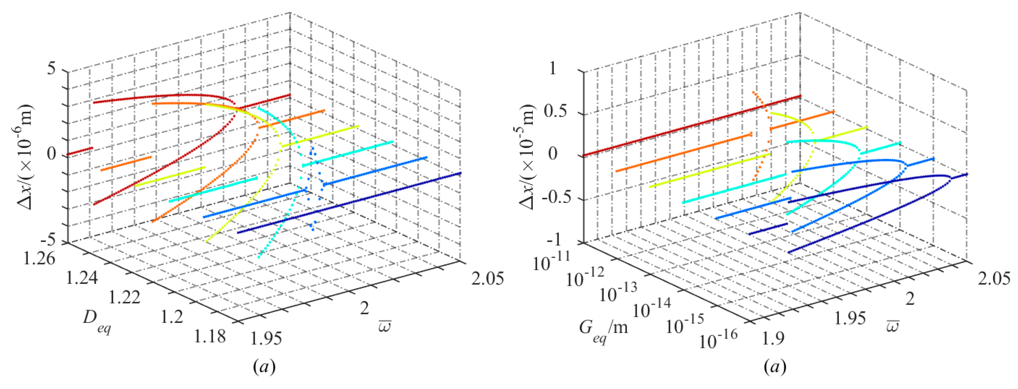
The effect of D_eq on nonlinear response is compared with the one of G_eq. Figure 12 depicts that with the increase of D_eq or decrease of G_eq, three different regions appear in succession on the bifurcation diagrams: 1T-period motion, 2T-period motion, and 1T-period motion. As noted above, critical values D_eq = 1.18 and G_eq = 10⁻¹¹ m can be found for $\overline{F}=0.9\times {10}^{-6}\mathrm{m}$ and $\overline{F}=1.1\times {10}^{-6}\mathrm{m}$ respectively. Doubling bifurcations both occur just before $\overline{\omega }=2$ and midpoints of 2T-period motion regions both move to the negative direction in Figure 12a,b. When the excitation frequency is out of the region of the 2T-period response, the change in displacement is slight and the dynamic behavior becomes relatively stable.

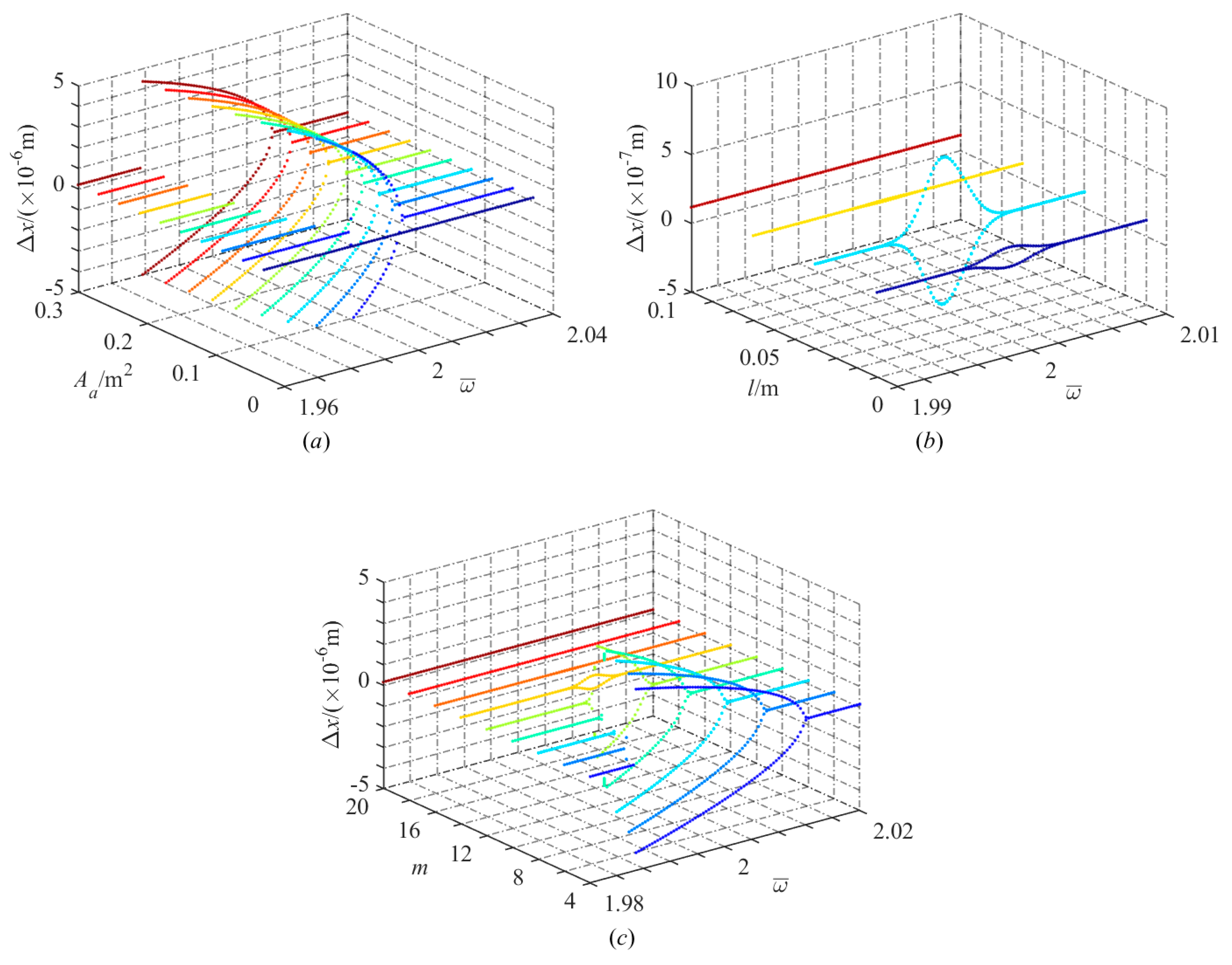
5.4. Effect of Other Structural Parameters on Nonlinear Response

The apparent contact area, thickness, and number of bolts are key parameters in the design of the bolt joint. Influences of the three parameters on the vibration of the system were studied. As $\overline{\omega }$ is increased in the neighborhood of 2, a transition from 1T-period motion to 2T-period motion, and finally back to 1T-period motion again can be observed under certain conditions, i.e., $A_a>0.03{\mathrm{m}}^2$ for $\overline{F}={10}^{-6}\mathrm{m}$, $l>0.1\mathrm{m}$ for $\overline{F}=0.59\times {10}^{-6}\mathrm{m}$ and $m<18$ for $\overline{F}=0.8\times {10}^{-6}\mathrm{m}$, are illustrated in Figure 13a–c, respectively. With the increase of A_a or decrease of m, the 2T-period motion regions are enlarged. However, the width of the region changes monotonously with the thickness l, which is presumed to be a convex function. That is, the bolted joints tend to be stable if A_a decreases, m increases or l increases after a certain value. Moreover, midpoints of 2T-period motion regions are not sensitive to the apparent contact area, thickness, and number of bolts.

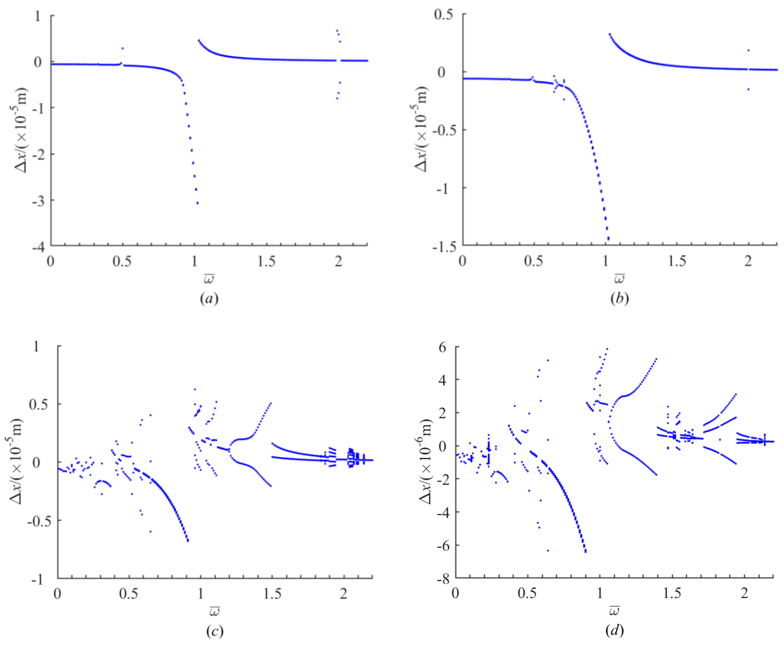
5.5. Effect of Bolt Pre-Tightening on Nonlinear Response

The pretension force of bolts performs a great influence on the mechanical capacity of the system. In order to analyze the effect of the bolt pre-tightening on dynamic behaviors, bifurcation diagrams are presented for f_pre = 3, 1, 0.1, and 0 kN. As demonstrated in Figure 14a, there appears a 2T-period response from frequency ratio $\overline{\omega }=1.99$ to $\overline{\omega }=2.01$. When f_pre is decreased to 1 kN, the 2T-period motion region becomes narrow can be seen in Figure 14b. Meanwhile, another region of 2T-period response and a region of 3T-period response occur near $\overline{\omega }=0.65$ and $\overline{\omega }=0.71$, respectively. Figure 14c depicts that as f_pre continues to increase, more bifurcation points separate the region of excitation frequency into a number of stages. In some stages, 4T-, 5T-, 7T-, 8T-, 15T-, 30T-, and 40T- period responses are observed, which shows the appearance of subharmonics. With the further decrease of f_pre, chaotic behavior at $\overline{\omega }=0.23$ is clearly visible in Figure 14d.

6. Conclusions

The surface topography has a significant effect on the vibration characteristics and stability of the contact interface system. In this article, an improved model of contact stiffness is developed to supply a study foundation. Furthermore, based on the contact model, a single-freedom dynamic model of the joint parts with the consideration of fractal surface has been established. In addition, the influences of excitation force and key design parameters of the machined bolt joint interface are discussed by amplitude–frequency curves, bifurcation diagrams, 3-D frequency spectrums, time histories, phase plane diagrams, and Poincare sections. Theconclusions are as follows:

• The stiffness of the system increases nonlinearly with the deflection, which shows the hardening type nonlinearity in the positive direction and the softening type nonlinearity in the opposite direction. However, the system performs softening behavior under harmonic excitation.
• The surface topography is controlled by fractal parameters D and G. With the increase of D or the decrease of G, the stiffness increases if the displacement is positive, and the bolt joint becomes relatively unstable.
• The system is sensitive and unstable when it has a higher excitation force. When the bolt pre-tightening is controlled and the interface has not been separated, the joint parts present a poor stability with a smaller bolt pre-tightening force. Moreover, as the apparent contact area increases or the number of bolts decreases, subharmonics appear.