Author Contributions
Conceptualization, H.A.F. and A.A.E.A.A.; Methodology, R.W.Z., H.A.F. and A.A.E.A.A.; Software, R.W.Z., H.A.F. and A.A.E.A.; Validation, H.A.F., A.A.E.A. and M.H.A.; Formal Analysis, H.A.F. and A.A.E.A.; Investigation, R.W.Z.; Resources, R.W.Z., H.A.F. and A.A.E.A.; Data Curation, R.W.Z.; Writing—Original Draft Preparation, R.W.Z.; Writing—Review and Editing, H.A.F., A.A.E.A. and M.H.A.; Visualization, R.W.Z., H.A.F. and A.A.E.A.; Supervision, H.A.F., A.A.E.A. and M.H.A.; Project Administration, R.W.Z., H.A.F. and A.A.E.A.
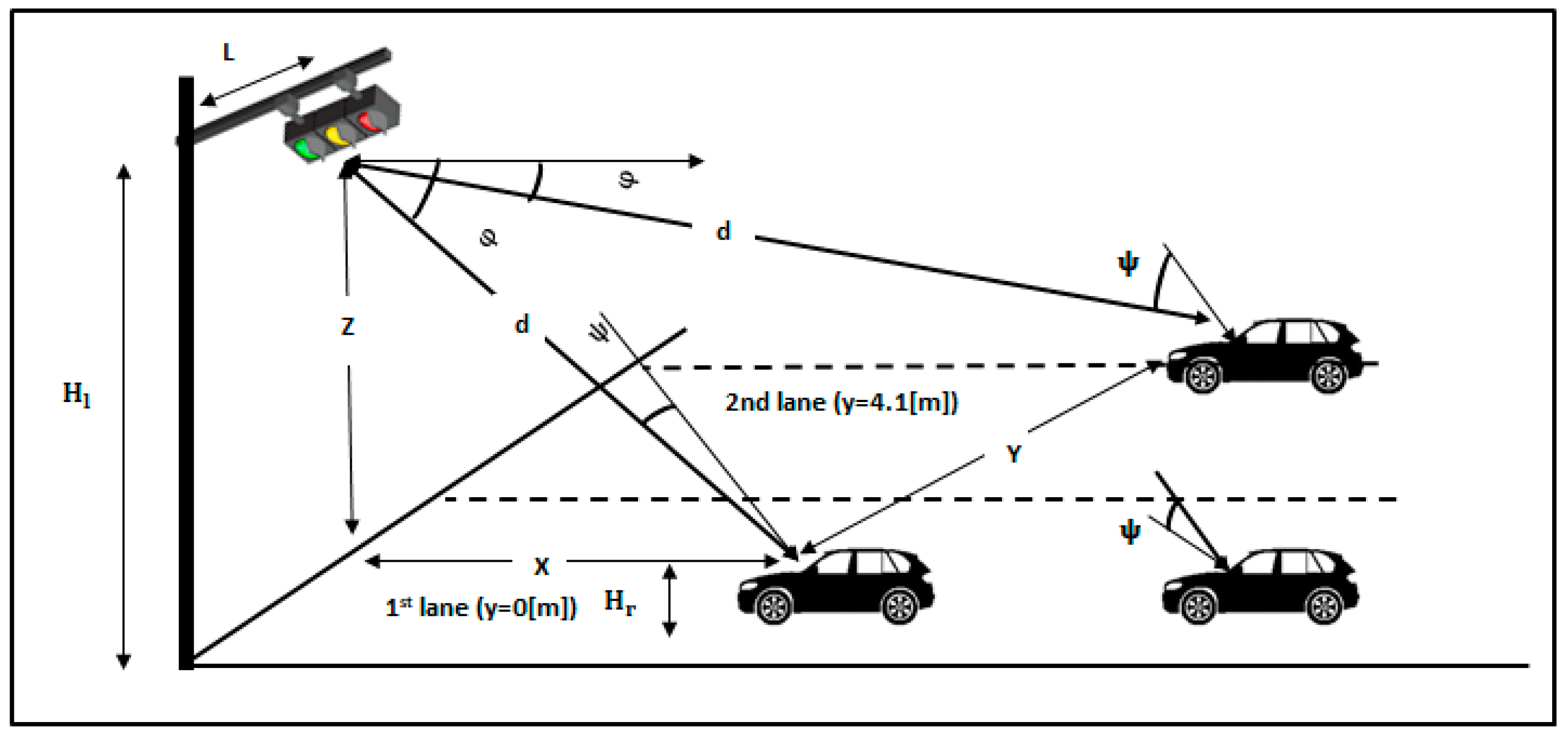
Figure 1.
Two-lane traffic light system model [
12].
Figure 1.
Two-lane traffic light system model [
12].
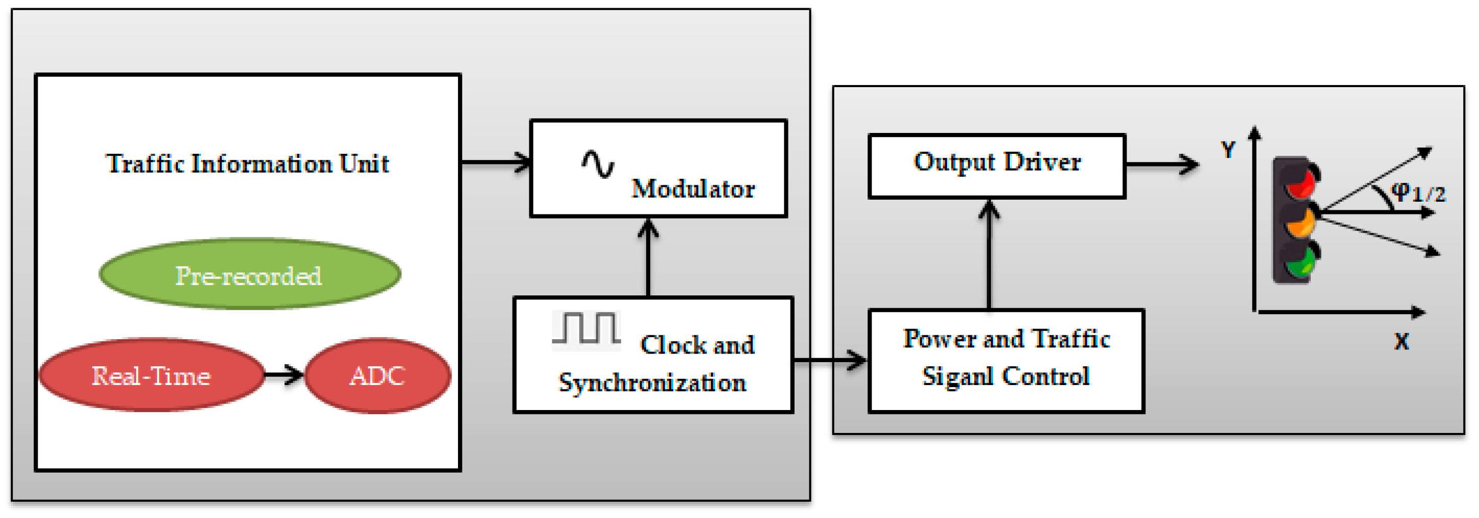
Figure 2.
Light-emitting diode (LED)-based traffic light block diagram.
Figure 2.
Light-emitting diode (LED)-based traffic light block diagram.
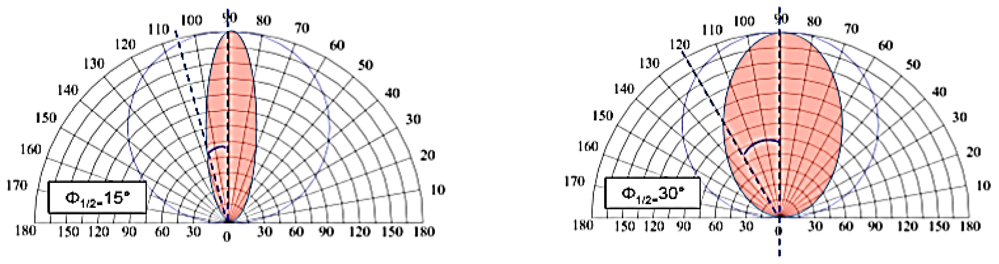
Figure 3.
LED Lambertian emission pattern and coverage area represented by and index m.
Figure 3.
LED Lambertian emission pattern and coverage area represented by and index m.
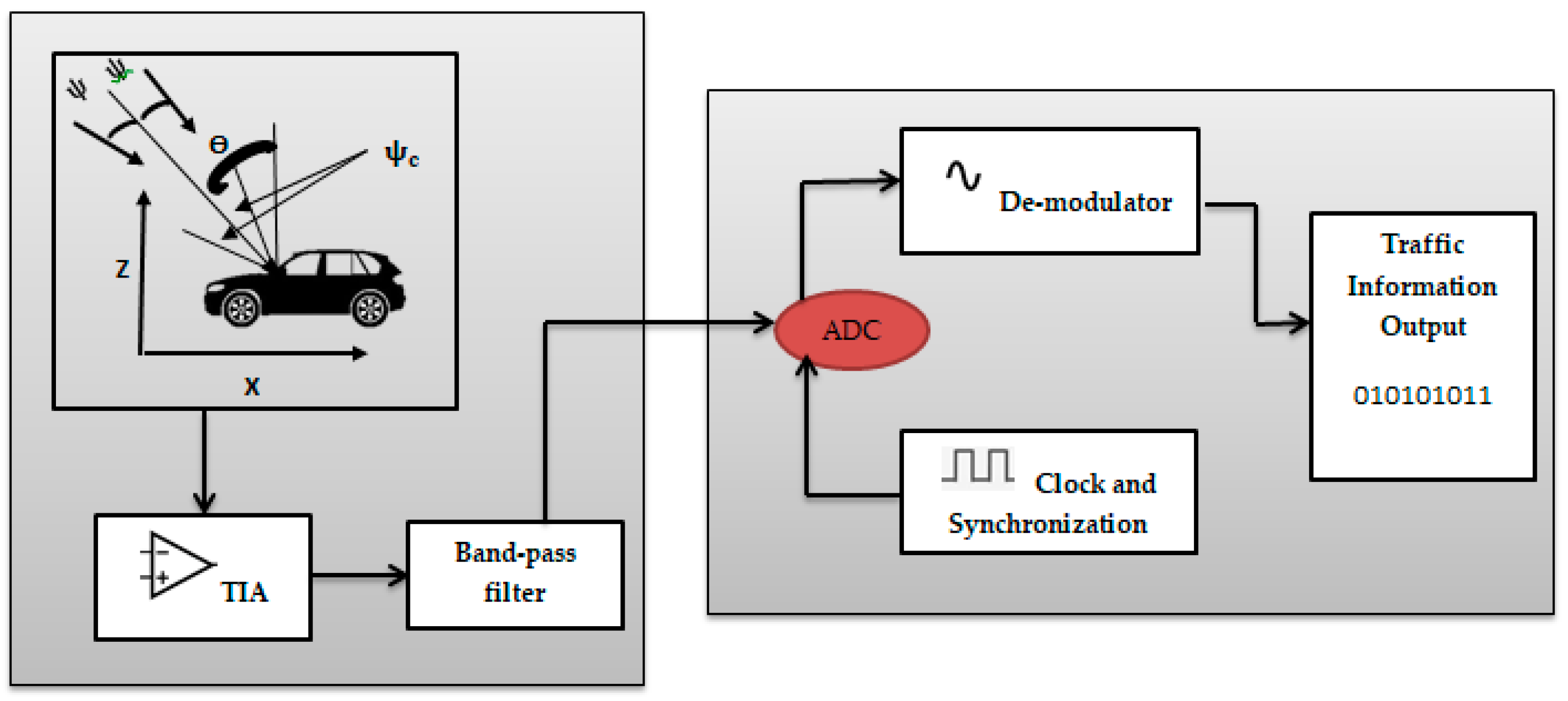
Figure 4.
Visible light communication (VLC) receiver block diagram.
Figure 4.
Visible light communication (VLC) receiver block diagram.
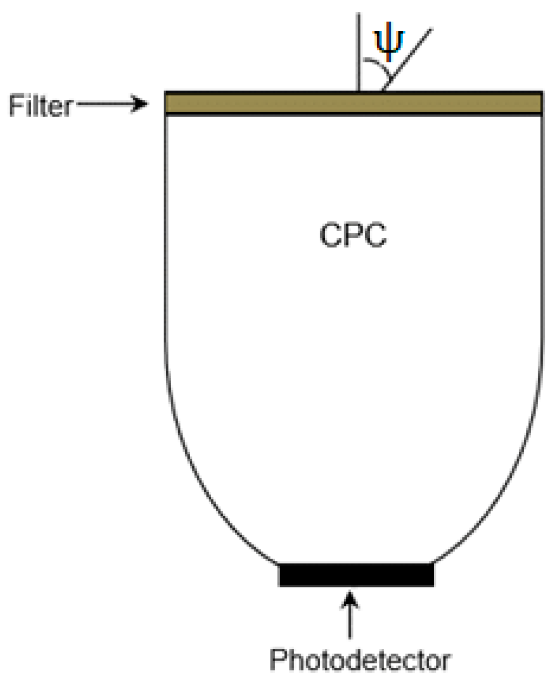
Figure 5.
The compound parabolic concentrator (CPC) non-imaging concentrator model.
Figure 5.
The compound parabolic concentrator (CPC) non-imaging concentrator model.
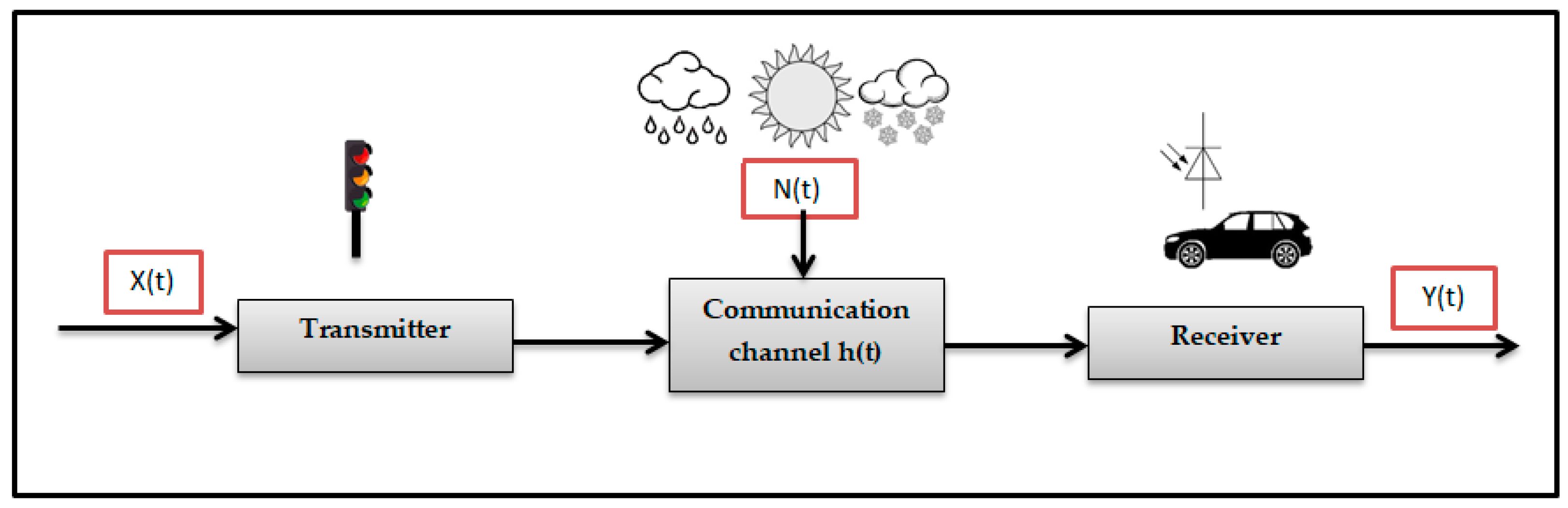
Figure 6.
Simplified outdoor VLC model in an intelligent transport system (ITS).
Figure 6.
Simplified outdoor VLC model in an intelligent transport system (ITS).
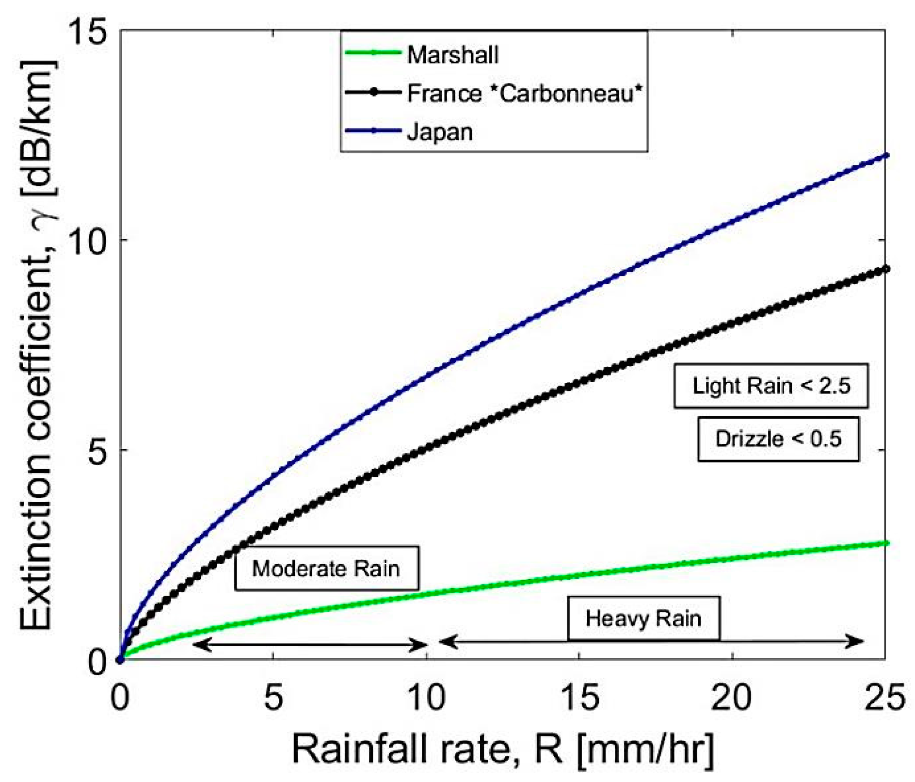
Figure 7.
Extinction coefficient vs. rainfall precipitation rate for different models.
Figure 7.
Extinction coefficient vs. rainfall precipitation rate for different models.
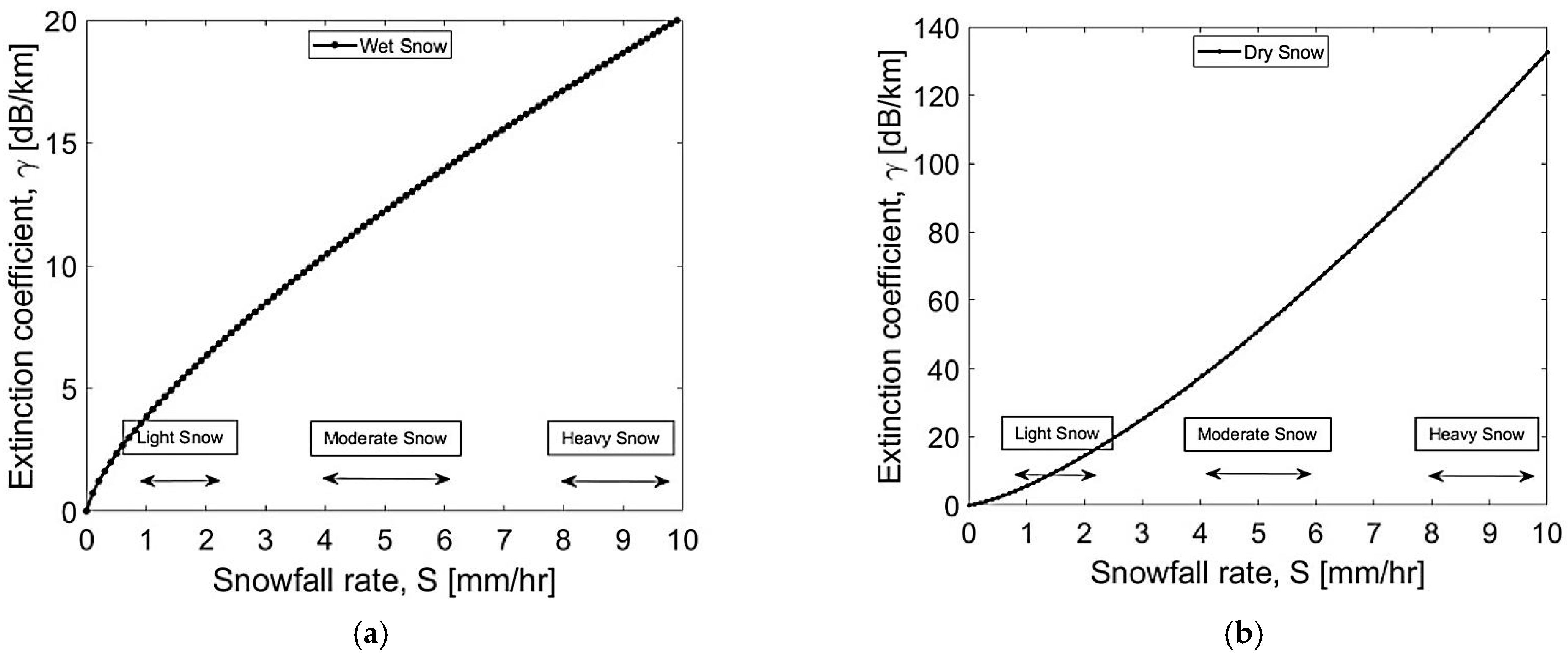
Figure 8.
Extinction coefficient vs. snowfall precipitation rate for λ = 505 nm (a) wet snow (b) dry snow.
Figure 8.
Extinction coefficient vs. snowfall precipitation rate for λ = 505 nm (a) wet snow (b) dry snow.
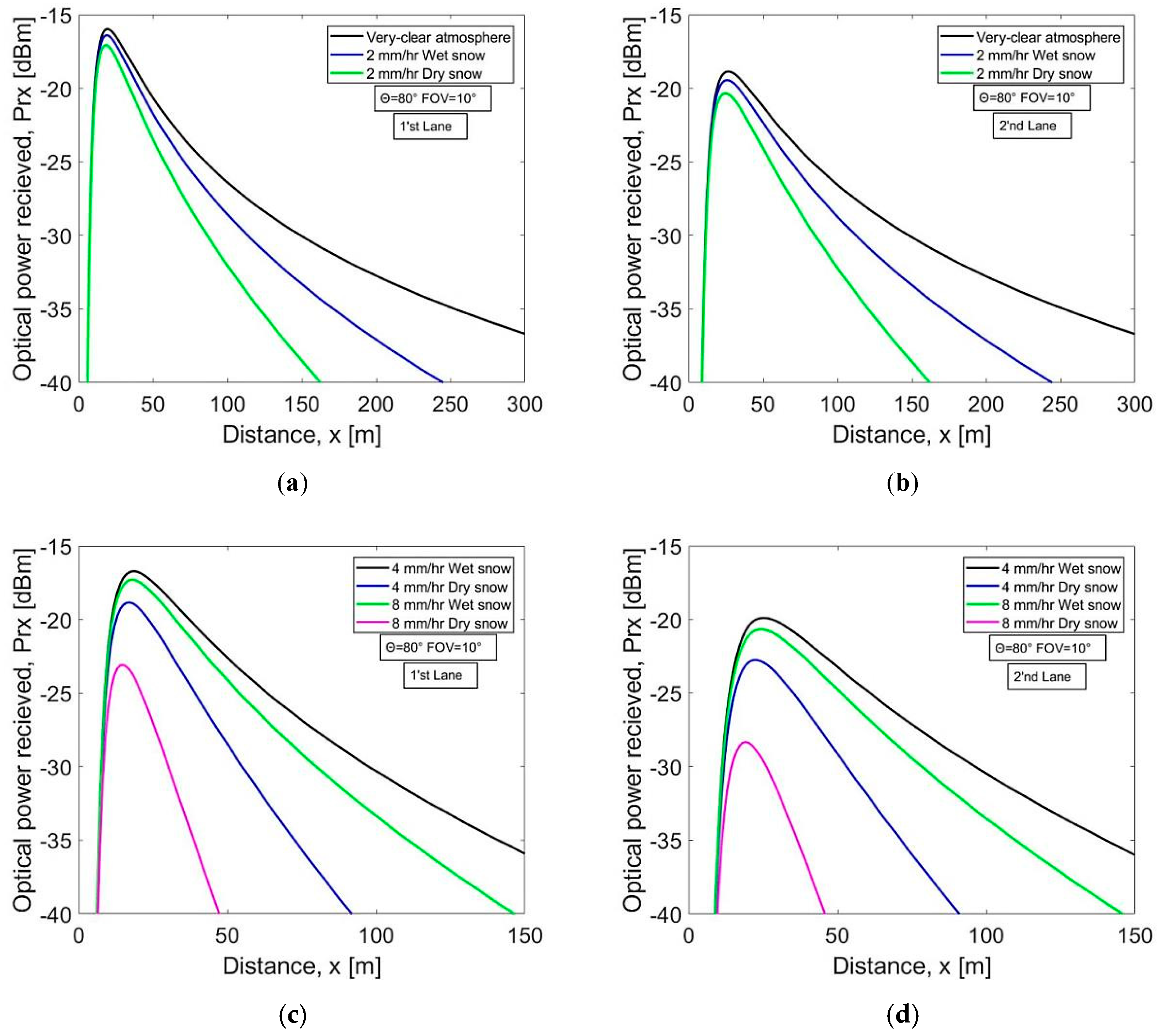
Figure 9.
Optical power received vs. distance for (a) very clear weather and 2 mm/h wet, dry snow in the first lane (b) very clear weather and 2 mm/h wet, dry snow in the second lane (c) 4, 8 mm/h wet, dry snow in the first lane (d) 4, 8 mm/h wet, dry snow in the second lane.
Figure 9.
Optical power received vs. distance for (a) very clear weather and 2 mm/h wet, dry snow in the first lane (b) very clear weather and 2 mm/h wet, dry snow in the second lane (c) 4, 8 mm/h wet, dry snow in the first lane (d) 4, 8 mm/h wet, dry snow in the second lane.
Figure 10.
Optical power received vs. distance for (a) very clear weather and different rain models at 25 mm/h in the first lane, (b) very clear weather and different rain models at 25 mm/h in the second lane, (c) different rain models at 10 mm/h in the first lane, (d) different rain models at 10 mm/h in the second lane, (e) different rain models at 2 mm/h in the first lane, and (f) different rain models at 2 mm/h in the second lane.
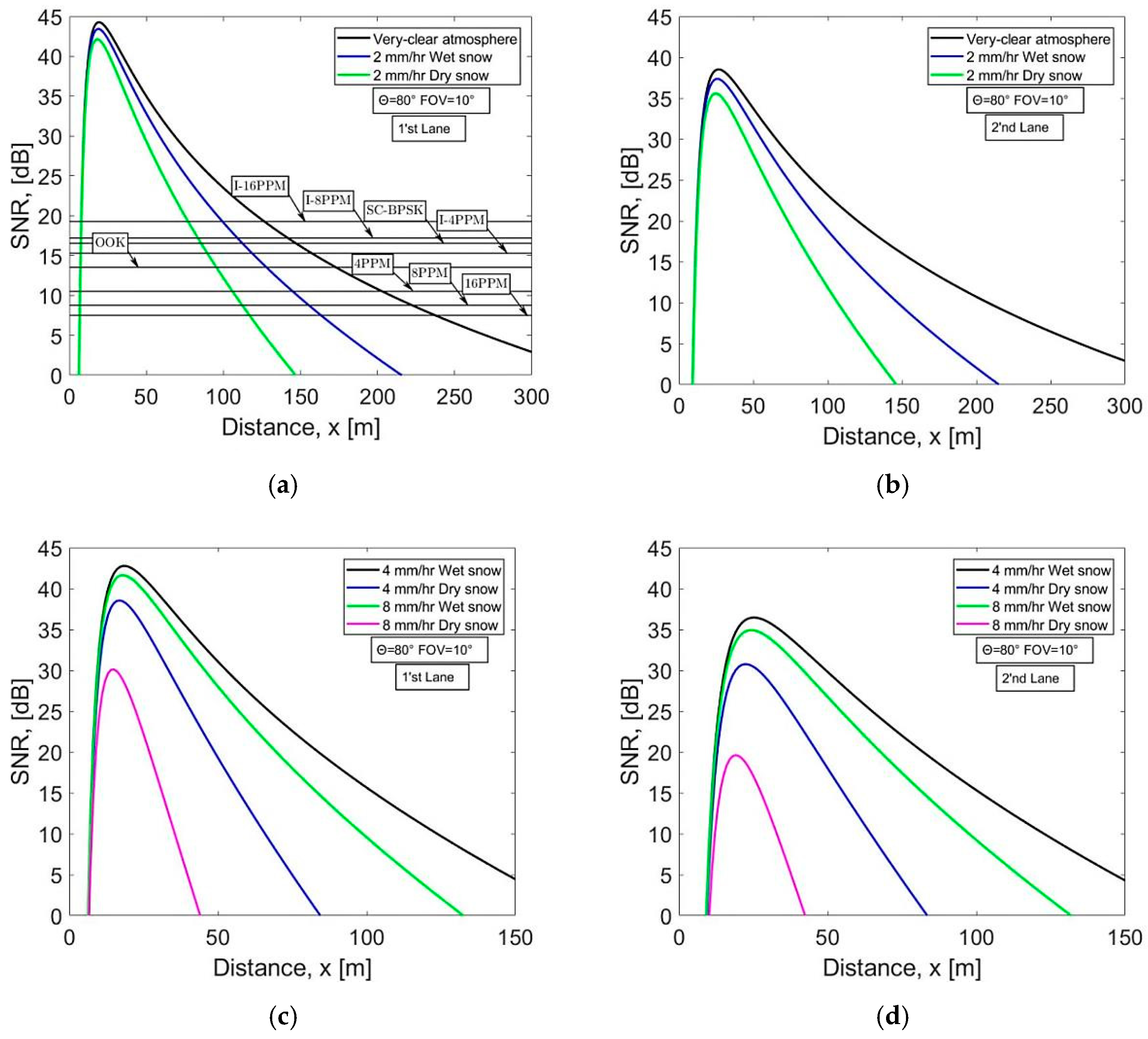
Figure 11.
Signal-to-noise ratio vs. distance for (a) very clear weather and 2 mm/h wet, dry snow in the first lane, (b) very clear weather and 2 mm/h wet, dry snow in the second lane, (c) 4, 8 mm/h wet, dry snow in the first lane, and (d) 4, 8 mm/h wet, dry snow in the second lane.
Figure 11.
Signal-to-noise ratio vs. distance for (a) very clear weather and 2 mm/h wet, dry snow in the first lane, (b) very clear weather and 2 mm/h wet, dry snow in the second lane, (c) 4, 8 mm/h wet, dry snow in the first lane, and (d) 4, 8 mm/h wet, dry snow in the second lane.
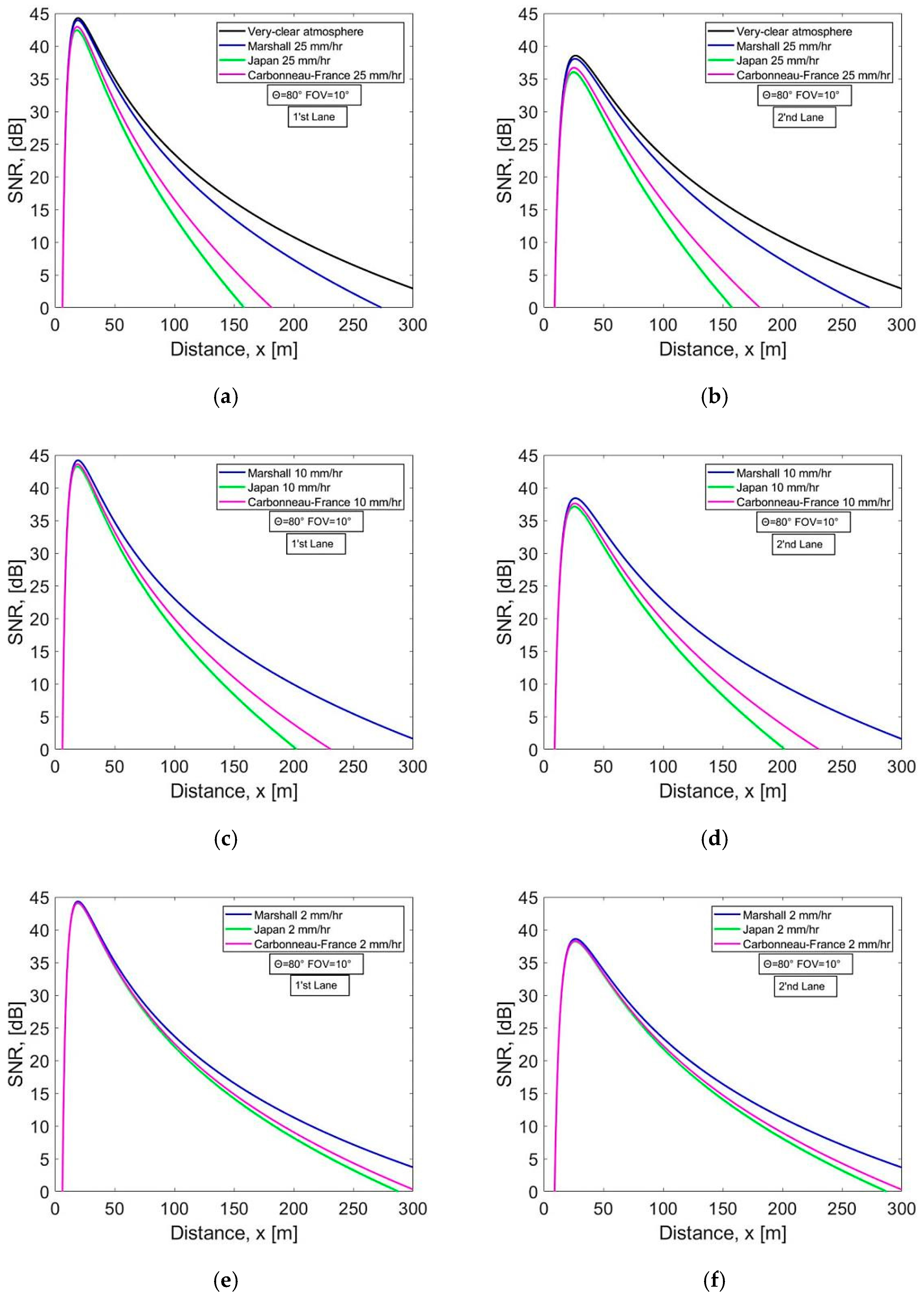
Figure 12.
Signal-to-noise ratio vs. distance for (a) very clear weather and different rain models at 25 mm/h in the first lane, (b) very clear weather and different rain models at 25 mm/h in the second lane, (c) different rain models at 10 mm/h in the first lane, (d) different rain models at 10 mm/h in the second lane, (e) different rain models at 2 mm/h in the first lane, and (f) different rain models at 2 mm/h in the second lane.
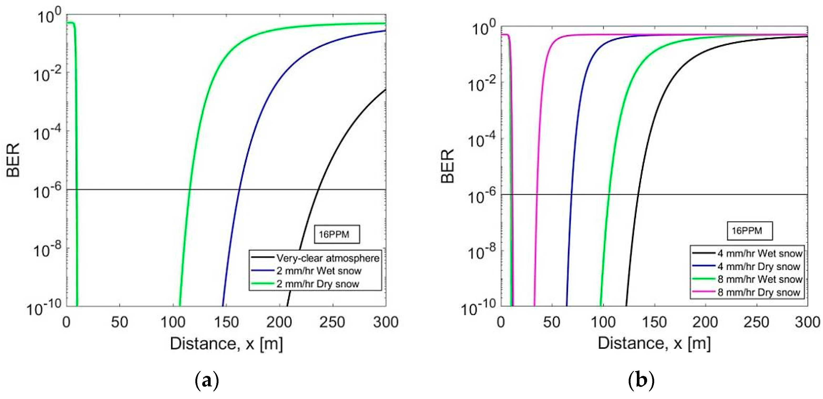
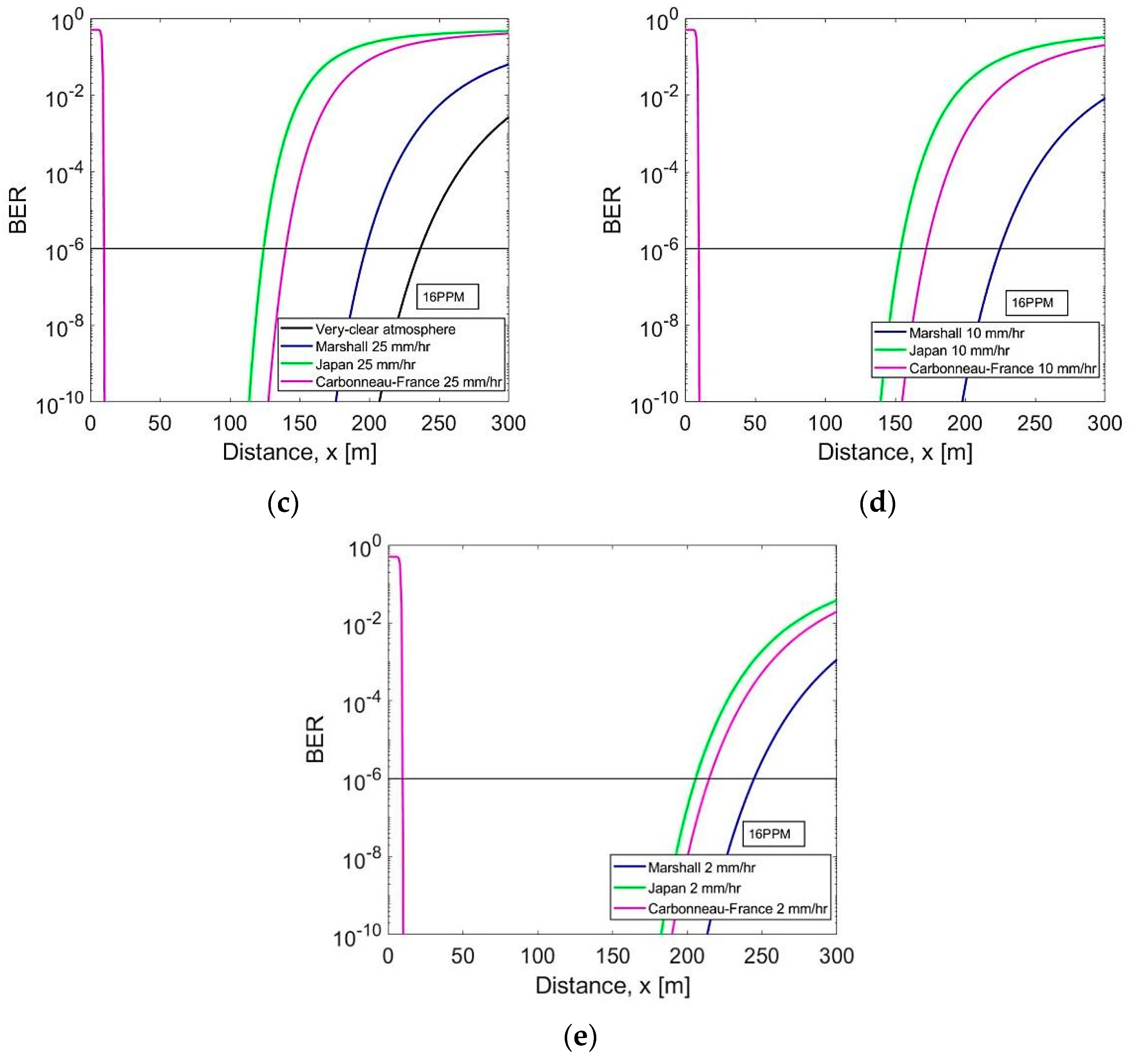
Figure 13.
Bit error rate vs. distance under 16PPM scheme for (a) very clear weather and 2 mm/h wet, dry snow, (b) 4, 8 mm/h wet, dry snow, (c) very clear weather and different rain models at 25 mm/h, (d) different rain models at 10 mm/h, and (e) different rain models at 2 mm/h.
Figure 13.
Bit error rate vs. distance under 16PPM scheme for (a) very clear weather and 2 mm/h wet, dry snow, (b) 4, 8 mm/h wet, dry snow, (c) very clear weather and different rain models at 25 mm/h, (d) different rain models at 10 mm/h, and (e) different rain models at 2 mm/h.
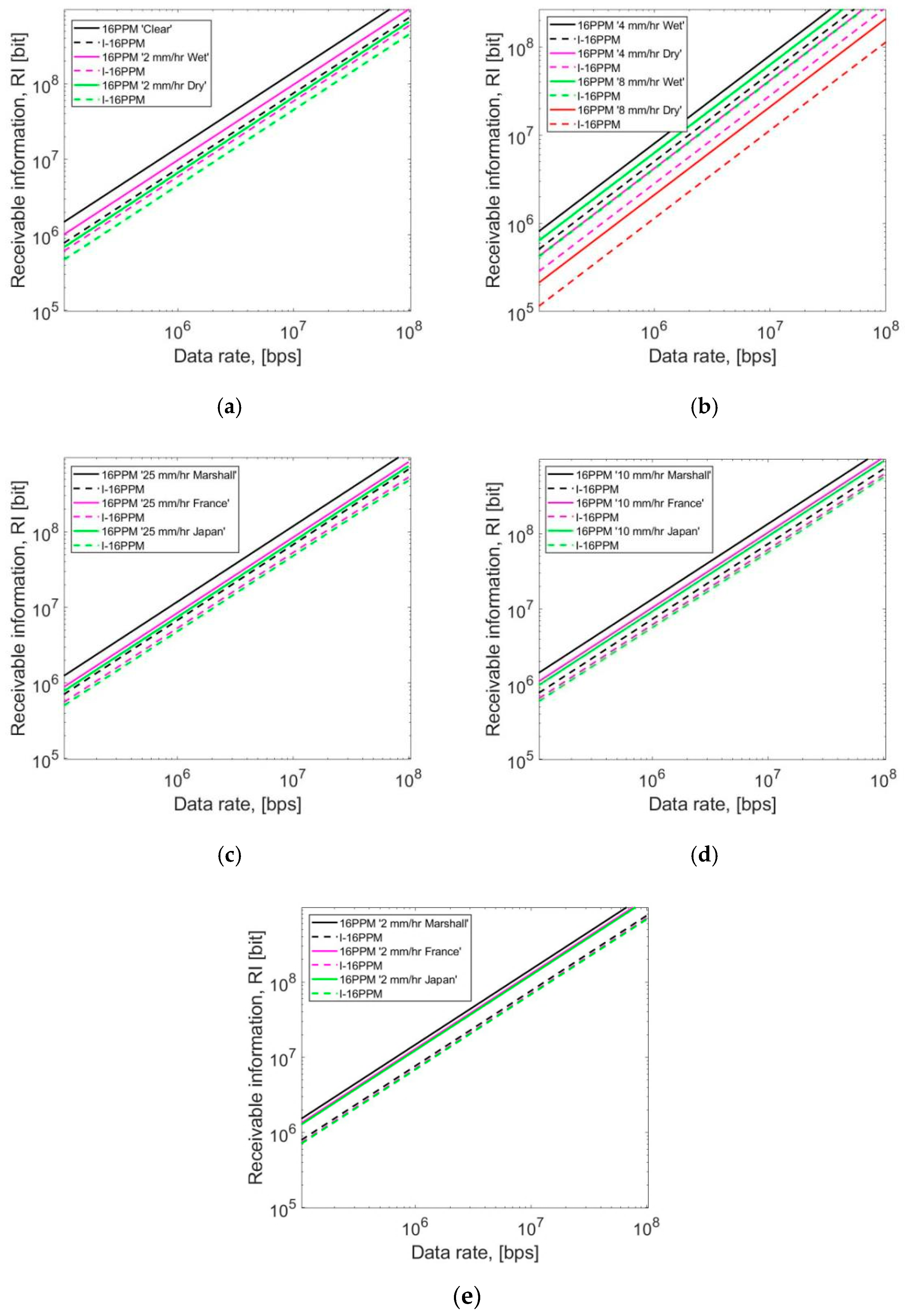
Figure 14.
Received information (RI) vs. data rate under 16PPM and I-16 PPM schemes for (a) very clear weather and 2 mm/h wet, dry snow, (b) 4, 8 mm/h wet, dry snow, (c) different rain models at 25 mm/h, (d) different rain models at 10 mm/h, and (e) different rain models at 2 mm/h.
Figure 14.
Received information (RI) vs. data rate under 16PPM and I-16 PPM schemes for (a) very clear weather and 2 mm/h wet, dry snow, (b) 4, 8 mm/h wet, dry snow, (c) different rain models at 25 mm/h, (d) different rain models at 10 mm/h, and (e) different rain models at 2 mm/h.
Table 1.
System parameters [
12]. FOV: field of view.
Table 1.
System parameters [
12]. FOV: field of view.
| Parameter | Symbol | Value |
|---|
| Length of traffic arm | L | 2.0 [m] |
| Height of traffic light | | 5.3 [m] |
| Height of receiver | | 1.0 [m] |
| Distance in lane direction | X | [m] |
| Distance in width direction | Y | [m] |
| Difference between and | Z | 4.3 [m] |
| Width of lane | | 3.5 [m] |
| Width of vehicle | | 1.8 [m] |
| Distance between transmitter and receiver | d | [m] |
| Half power semi-angle | | 15 [°] |
| Vertical inclination | θ | 0° ≤ θ ≤ 90° |
| FOV of receiver | | 0° ≤ ≤ 90° |
Table 2.
Attenuation parameters due to rain.
Table 2.
Attenuation parameters due to rain.
| Location/Model | a | b |
|---|
| Marshall and Palmer | 0.365 | 0.63 |
| Carbonneau–France | 1.076 | 0.67 |
| Japan | 1.58 | 0.63 |
Table 3.
Attenuation parameters due to snow.
Table 3.
Attenuation parameters due to snow.
| Snow Type | a | b |
|---|
| Wet | 0.000102 * λ + 3.79 | 0.72 |
| Dry | 0.0000542 * λ + 5.50 | 1.38 |
Table 4.
Necessary signal-to-noise ratio (SNR) corresponding to target bit error rate (BER) = 10−6. OOK: ON–OFF Keying, SC-BPSK: Subcarrier Binary Phase-Shift Keying, L-PPM: L-Pulse Position Modulation, I-LPPM: Inverse L-Pulse Position Modulation.
Table 4.
Necessary signal-to-noise ratio (SNR) corresponding to target bit error rate (BER) = 10−6. OOK: ON–OFF Keying, SC-BPSK: Subcarrier Binary Phase-Shift Keying, L-PPM: L-Pulse Position Modulation, I-LPPM: Inverse L-Pulse Position Modulation.
| Modulation Scheme | Minimum SNR (dB) |
|---|
| OOK | 13.53 |
| SC-BPSK | 16.54 |
| L-PPM | 4PPM | 10.52 |
| 8PPM | 8.76 |
| 16PPM | 7.5 |
| I-LPPM | I-4PPM | 15.29 |
| I-8PPM | 17.21 |
| I-16PPM | 19.27 |
Table 5.
Attenuation for various weather conditions.
Table 5.
Attenuation for various weather conditions.
| Weather Condition | Attenuation [dB/km] for Different Precipitation Rates |
|---|
| Snow | Light | Moderate | Heavy |
| 2 mm/h | 4 mm/h | 8 mm/h |
| Wet | 6 | 10 | 17 |
| Dry | 14 | 37 | 97 |
| Rain | Light | Moderate | Heavy |
| 2 mm/h | 10 mm/h | 25 mm/h |
| Marshall model | 0.7 | 1.5 | 3 |
| France model by Carbonneau | 2 | 5 | 9 |
| Japan model | 2.5 | 7 | 12 |
| Very clear | 0.911 |
Table 6.
Numerical analysis parameters [
13]. FET: field-effect transistor.
Table 6.
Numerical analysis parameters [
13]. FET: field-effect transistor.
| Parameter | Symbol | Value |
|---|
| Transmission optical power | | 314 [mW] |
| Detector physical area | A | 0.79 [] |
| Gain of optical filter | (ψ) | 1.0 |
| Refractive index of concentrator | n | 1.7 |
| Electron charge | q | 1.602e-19 [C] |
| Photodetector responsivity | r | 0.35 [A/W] |
| Boltzmann’s constant | | 1.3811e-23 [J/K] |
| Absolute temperature | T | 298 [°K] |
| Open-loop voltage gain | G | 10 |
| FET transconductance | | 30 [mS] |
| FET channel noise factor | | 1.5 |
| Bandwidth of band-pass optical filter | | 10 [nm] |
| Background irradiance per unit bandwidth | | 5.8 [μW/ |
| Capacitance per unit area | | 112 [pF/cm2] |
| Noise bandwidth factors | | 0.562 |
| 0.868 |
| Wavelength of LED | λ | 505 [nm] |
| Vehicle velocity | | 60 [km/h] |
| Transmission data rate | | 10 M [bit/s] |
Table 7.
Maximum distance for different modulation schemes under various weather conditions.
Table 7.
Maximum distance for different modulation schemes under various weather conditions.
| Weather Condition | Maximum Distance [m] |
|---|
| OOK | SC-BPSK | 4PPM | I-4PPM | 8PPM | I-8PPM | 16PPM | I-16PPM |
|---|
| Very-Clear | 173 | 123 | 202 | 156 | 222 | 140 | 237 | 125 |
| Wet snow | Precipitation level mm/h | 2 | 128 | 97 | 144 | 117 | 155 | 107 | 162 | 98 |
| 4 | 108 | 84 | 120 | 100 | 128 | 92 | 134 | 84 |
| 8 | 88 | 69 | 96 | 81 | 101 | 75 | 105 | 69 |
| Dry Snow | Precipitation level mm/h | 2 | 95 | 75 | 105 | 89 | 111 | 82 | 116 | 75 |
| 4 | 60 | 47 | 63 | 54 | 66 | 51 | 69 | 47 |
| 8 | 32 | 20 | 32 | 27 | 34 | 24 | 35 | 19 |
| Marshall | Precipitation level mm/h | 2 | 177 | 125 | 207 | 159 | 228 | 143 | 244 | 127 |
| 10 | 166 | 119 | 192 | 150 | 211 | 136 | 224 | 121 |
| 25 | 150 | 110 | 172 | 137 | 186 | 125 | 197 | 112 |
| France | Precipitation level mm/h | 2 | 160 | 116 | 185 | 145 | 201 | 131 | 214 | 117 |
| 10 | 134 | 100 | 151 | 123 | 163 | 112 | 172 | 102 |
| 25 | 113 | 87 | 125 | 104 | 134 | 96 | 140 | 88 |
| Japan | Precipitation level mm/h | 2 | 154 | 113 | 178 | 141 | 193 | 127 | 205 | 114 |
| 10 | 112 | 93 | 137 | 112 | 147 | 103 | 154 | 94 |
| 25 | 102 | 79 | 112 | 94 | 119 | 87 | 124 | 80 |


