Fast Implicit Surface Reconstruction for the Radial Basis Functions Interpolant


Abstract
1. Introduction
2. Related Works
3. Implicit Function
4. Fast Evaluation
4.1. Black-Box FMM
4.2. Single Point FMM
5. Fast Reconstruction
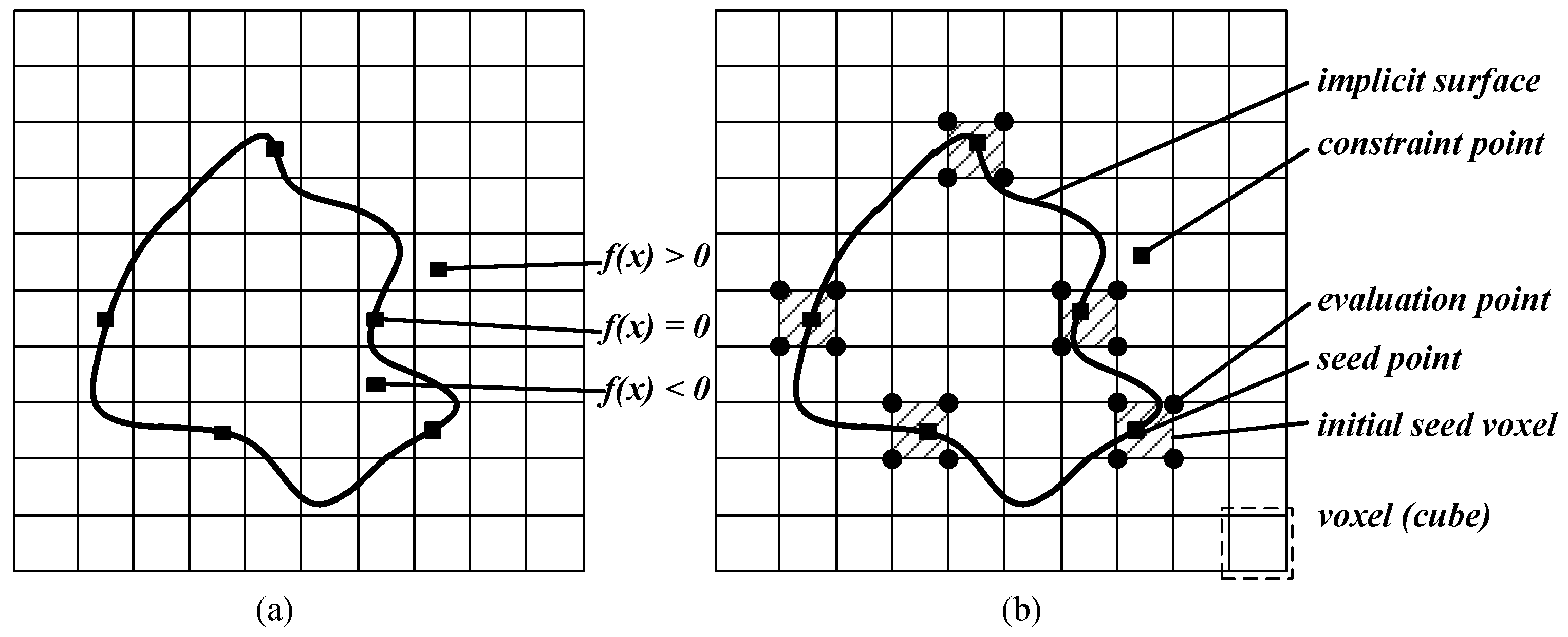
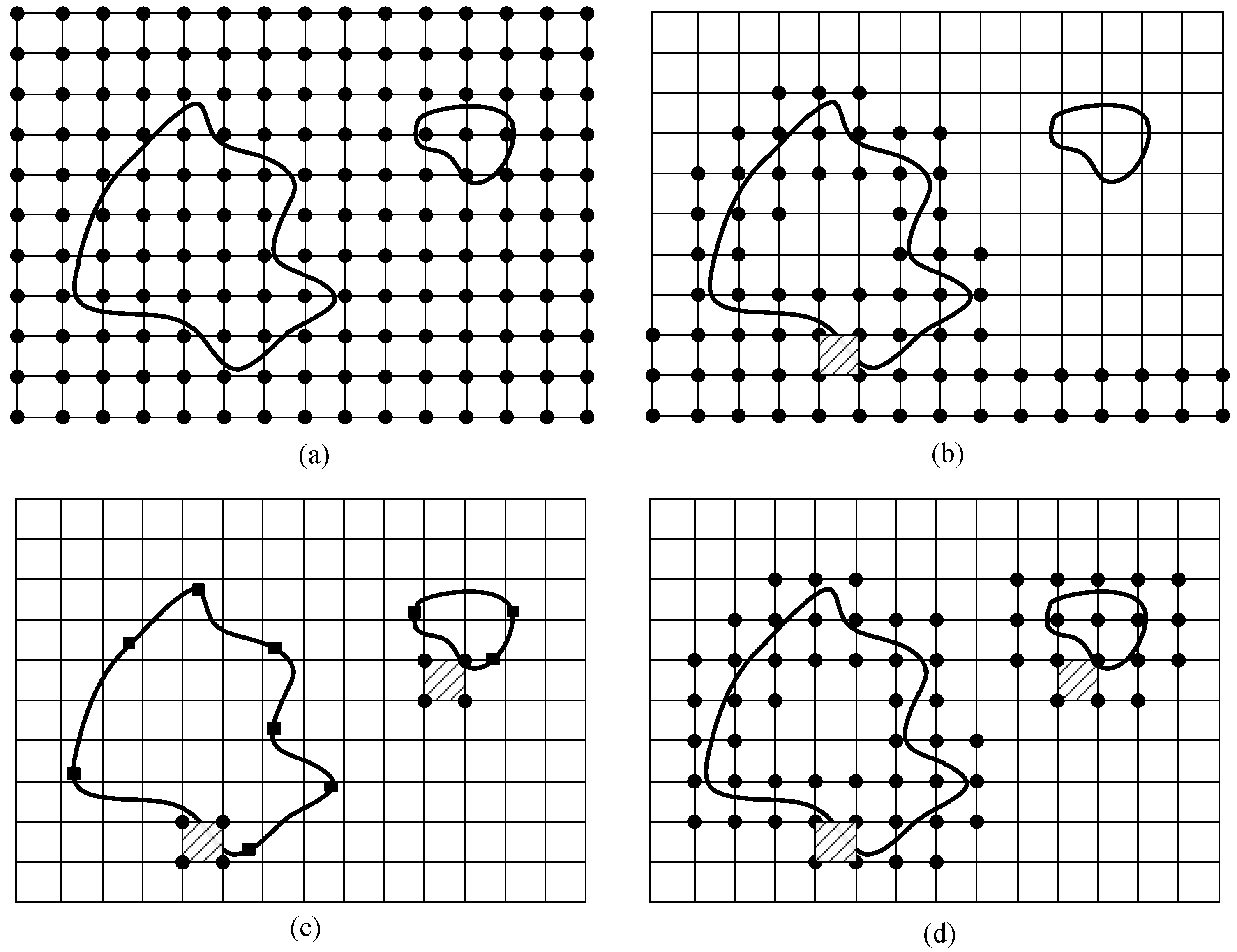
5.1. Voxel Growing
5.2. Leaf Growing
6. Numerical Results
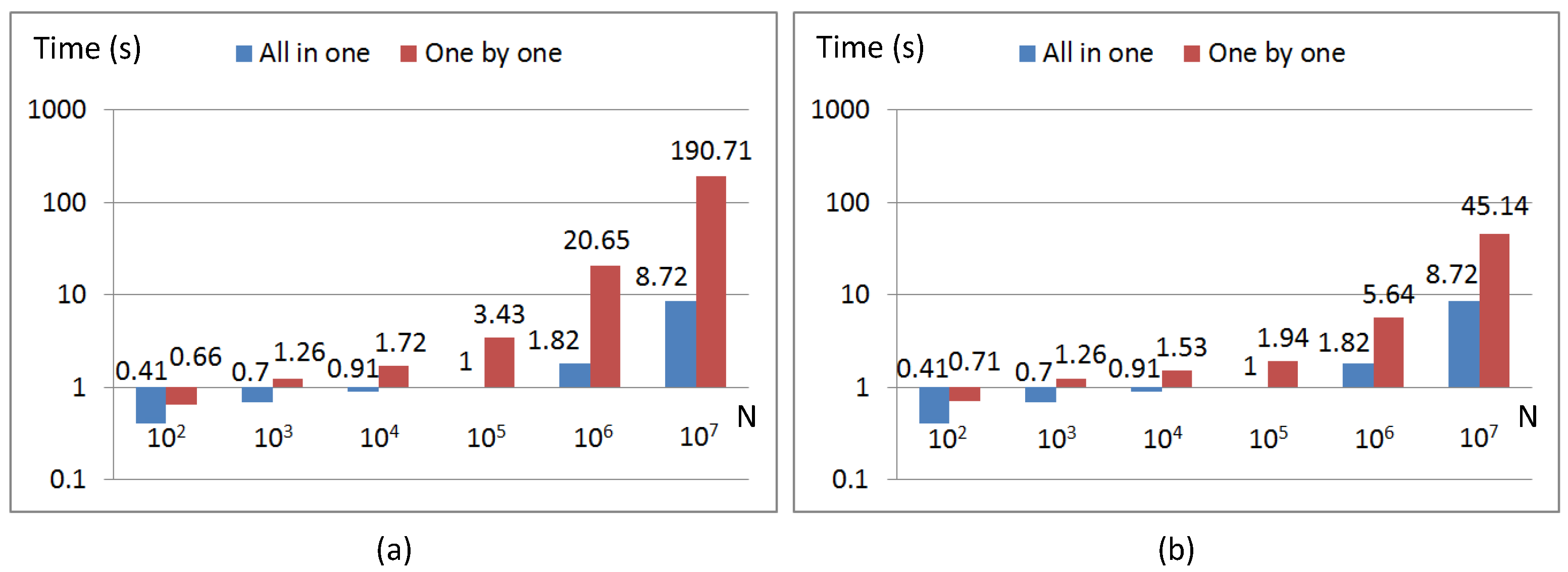
6.1. Performance
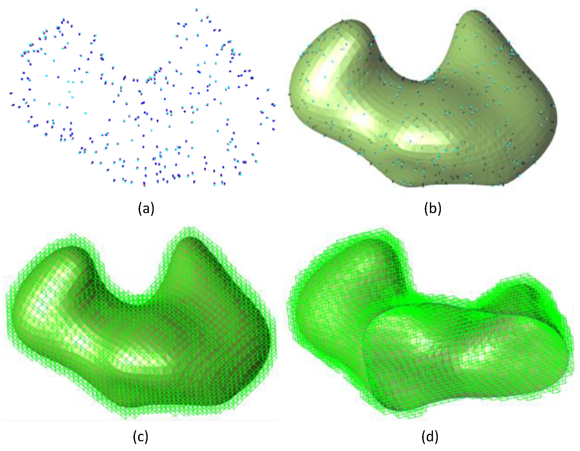
6.2. Case Studies
7. Conclusions and Discussion
Author Contributions
Funding
Acknowledgments
Conflicts of Interest
References
- De Boer, A.; Van der Schoot, M.; Bijl, H. Mesh deformation based on radial basis function interpolation. Comput. Struct. 2007, 85, 784–795. [Google Scholar] [CrossRef]
- Majdisova, Z.; Skala, V. Radial basis function approximations: Comparison and applications. App. Math. Model. 2017, 51, 728–743. [Google Scholar] [CrossRef]
- Carr, J.C.; Beatson, R.K.; Cherrie, J.B.; Mitchell, T.J.; Fright, W.R.; McCallum, B.C.; Evans, T.R. Reconstruction and representation of 3D objects with radial basis functions. In Proceedings of the 28th Annual Conference on Computer Graphics and Interactive Techniques, Los Angeles, CA, USA, 12–17 August 2001; pp. 67–76. [Google Scholar]
- Li, J.; Hon, Y. Domain decomposition for radial basis meshless methods. Numer. Methods Partial Differ. Equ. 2004, 20, 450–462. [Google Scholar] [CrossRef]
- Krese, B.; Perc, M.; Govekar, E. The dynamics of laser droplet generation. Chaos 2010, 20, 013129. [Google Scholar] [CrossRef]
- KRESE, B.; PERC, M.; Govekar, E. Experimental observation of a chaos-to-chaos transition in laser droplet generation. Int. J. Bifurcat. Chaos 2011, 21, 1689–1699. [Google Scholar] [CrossRef]
- Jessell, M.; Aillères, L.; De Kemp, E.; Lindsay, M.; Wellmann, J.; Hillier, M.; Laurent, G.; Carmichael, T.; Martin, R. Next generation three-dimensional geologic modeling and inversion. Econ. Geol. 2014, 18, 261–272. [Google Scholar]
- Calakli, F.; Taubin, G. SSD: Smooth signed distance surface reconstruction. Comput. Graph. Forum 2011, 30, 1993–2002. [Google Scholar] [CrossRef]
- Lorensen, W.E.; Cline, H.E. Marching cubes: A high resolution 3D surface construction algorithm. ACM SIGGRAPH Comput. Graph. 1987, 21, 163–169. [Google Scholar] [CrossRef]
- Newman, T.S.; Yi, H. A survey of the marching cubes algorithm. Comput. Graph. 2006, 30, 854–879. [Google Scholar] [CrossRef]
- Lee, T.Y.; Lin, C.H. Growing-cube isosurface extraction algorithm for medical volume data. Comput. Med. Imag. Grap. 2001, 25, 405–415. [Google Scholar] [CrossRef]
- Wang, X.; Niu, Y.; Tan, L.W.; Zhang, S.X. Improved marching cubes using novel adjacent lookup table and random sampling for medical object-specific 3D visualization. J. Softw. 2014, 9, 10. [Google Scholar] [CrossRef]
- Darve, E. The fast multipole method: Numerical implementation. J. Comput. Phys. 2000, 160, 195–240. [Google Scholar] [CrossRef]
- Greengard, L.; Rokhlin, V. A new version of the fast multipole method for the Laplace equation in three dimensions. Acta Numer. 1997, 6, 229–269. [Google Scholar] [CrossRef]
- Hoppe, H. Poisson surface reconstruction and its applications. In Proceedings of the 2008 ACM Symposium on Solid and physical modeling, New York, NY, USA, 2–4 June 2008; p. 10. [Google Scholar]
- Kazhdan, M.; Hoppe, H. Screened poisson surface reconstruction. ACM Trans. Graph. 2013, 32, 29. [Google Scholar] [CrossRef]
- Frank, T.; Tertois, A.L.; Mallet, J.L. 3D-reconstruction of complex geological interfaces from irregularly distributed and noisy point data. Comput. Geosci. 2007, 33, 932–943. [Google Scholar] [CrossRef]
- Mallet, J.L. Discrete modeling for natural objects. Math. Geosci. 1997, 29, 199–219. [Google Scholar] [CrossRef]
- Beatson, R.K.; Ong, W.; Rychkov, I. Faster fast evaluation of thin plate splines in two dimensions. J. Comput. Appl. Math. 2014, 261, 201–212. [Google Scholar] [CrossRef]
- Spivak, M.; Veerapaneni, S.K.; Greengard, L. The fast generalized Gauss transform. SIAM J. Sci. Comput. 2010, 32, 3092–3107. [Google Scholar] [CrossRef]
- Beatson, R.; Powell, M.J.D.; Tan, A. Fast evaluation of polyharmonic splines in three dimensions. IMA J. Numer. Anal. 2006, 27, 427–450. [Google Scholar] [CrossRef][Green Version]
- Ying, L. A kernel independent fast multipole algorithm for radial basis functions. J. Comput. Phys. 2006, 213, 451–457. [Google Scholar] [CrossRef]
- Fong, W.; Darve, E. The black-box fast multipole method. J. Comput. Phys. 2009, 228, 8712–8725. [Google Scholar] [CrossRef]
- Zhang, Q.; Zhao, Y.; Levesley, J. Adaptive radial basis function interpolation using an error indicator. Numer. Algorithms 2017, 76, 441–471. [Google Scholar] [CrossRef]
- Nielson, G.M. Dual marching cubes. In Proceedings of the IEEE Visualization 2004, Austin, TX, USA, 10–15 October 2004; pp. 489–496. [Google Scholar]
- Shu, R.; Zhou, C.; Kankanhalli, M.S. Adaptive marching cubes. Vis. Comput. 1995, 11, 202–217. [Google Scholar] [CrossRef]
- Congote, J.; Moreno, A.; Barandiaran, I.; Barandiaran, J.; Ruiz, O. Extending Marching Cubes with Adaptative Methods to obtain more accurate iso-surfaces. In Proceedings of the International Conference on Computer Vision, Imaging and Computer Graphics, Lisboa, Portugal, 5–8 February 2009; pp. 35–44. [Google Scholar]
- Wu, Z.; Sullivan, J.M., Jr. Multiple material marching cubes algorithm. Int. J. Numer. Meth. Eng. 2003, 58, 189–207. [Google Scholar] [CrossRef]
- Treece, G.M.; Prager, R.W.; Gee, A.H. Regularised marching tetrahedra: Improved iso-surface extraction. Comput. Graph. 1999, 23, 583–598. [Google Scholar] [CrossRef]
- Beatson, R.K.; Cherrie, J.B.; Mouat, C.T. Fast fitting of radial basis functions: Methods based on preconditioned GMRES iteration. Adv. Comput. Math. 1999, 11, 253–270. [Google Scholar] [CrossRef]
- Beatson, R.K.; Light, W.; Billings, S. Fast solution of the radial basis function interpolation equations: Domain decomposition methods. SIAM J. Sci. Comput. 2001, 22, 1717–1740. [Google Scholar] [CrossRef]
- Gumerov, N.A.; Duraiswami, R.; Borovikov, E.A. Data Structures, Optimal Choice of Parameters, and Complexity Results for Generalized Multilevel Fast Multipole Methods in d Dimensions; University of Maryland: College Park, MD, USA, 2003. [Google Scholar]
- Takahashi, T.; Cecka, C.; Darve, E. Optimization of the parallel black-box fast multipole method on CUDA. In Proceedings of the 2012 Innovative Parallel Computing (InPar), San Jose, CA, USA, 13–14 May 2012; pp. 1–14. [Google Scholar]


| Model | Evaluation Points | Time (Seconds) | |||||||
|---|---|---|---|---|---|---|---|---|---|
| MC | VG | LG | MC | VG | LG | ||||
| Figure 10a | 21,975 | 2.0 | 10 | 5,972,274 | 167,858 | 167,858 | 11.4 | 4.5 | 4.1 |
| Figure 10b | 21,792 | 2.0 | 10 | 16,310,430 | 422,615 | 422,615 | 19.1 | 8.2 | 7.5 |
| Figure 10c | 45,975 | 1.0 | 10 | 7,180,920 | 173,552 | 173,552 | 41.3 | 10.8 | 10.3 |
| Figure 11a | 29,770 | 1.0 | 10 | 44,498,160 | 759,525 | 759,525 | 61.7 | 14.5 | 12.7 |
| Figure 11b | 29,397 | 1.0 | 10 | 261,766,151 | 1,320,267 | 1,320,267 | 63.3 | 23.8 | 19.9 |
| Figure 11c | 19,065 | 3.0 | 10 | 56,107,920 | 738,284 | 738,284 | 73.2 | 11.8 | 10.6 |
© 2019 by the authors. Licensee MDPI, Basel, Switzerland. This article is an open access article distributed under the terms and conditions of the Creative Commons Attribution (CC BY) license (http://creativecommons.org/licenses/by/4.0/).
Share and Cite
Zhong, D.; Zhang, J.; Wang, L. Fast Implicit Surface Reconstruction for the Radial Basis Functions Interpolant. Appl. Sci. 2019, 9, 5335. https://doi.org/10.3390/app9245335
Zhong D, Zhang J, Wang L. Fast Implicit Surface Reconstruction for the Radial Basis Functions Interpolant. Applied Sciences. 2019; 9(24):5335. https://doi.org/10.3390/app9245335
Chicago/Turabian StyleZhong, Deyun, Ju Zhang, and Liguan Wang. 2019. "Fast Implicit Surface Reconstruction for the Radial Basis Functions Interpolant" Applied Sciences 9, no. 24: 5335. https://doi.org/10.3390/app9245335
APA StyleZhong, D., Zhang, J., & Wang, L. (2019). Fast Implicit Surface Reconstruction for the Radial Basis Functions Interpolant. Applied Sciences, 9(24), 5335. https://doi.org/10.3390/app9245335