New Satellite Selection Approach for GPS/BDS/GLONASS Kinematic Precise Point Positioning

Abstract

With the development of global satellite navigation systems, kinematic Precise Point Positioning (PPP) is facing the increasing computational load of instantaneous (single-epoch) processing due to more and more visible satellites. At this time, the satellite selection algorithm that can effectively reduce the computational complexity causes us to consider its application in GPS/BDS/GLONASS kinematic PPP. Considering the characteristics of different systems and satellite selection algorithms, we proposed a new satellite selection approach (NSS model) which includes three different satellite selection algorithms (maximum volume algorithm, fast-rotating partition satellite selection algorithm, and elevation partition satellite selection algorithm). Additionally, the inheritance of ambiguity was also proposed to solve the situation of constantly re-estimated integer ambiguity when the satellite selection algorithm is used in PPP. The results show that the NSS model had a centimeter-level positioning accuracy when the original PPP and optimal dilution of precision (DOP) algorithm solution were compared in kinematic PPP based on the data at five multi-GNSS Experiment (MGEX) stations. It can also reduce a huge amount of computation at the same time. Thus, the application of the NSS model is an effective method to reduce the computational complexity and guarantee the final positioning accuracy in GPS/BDS/GLONASS kinematic PPP.

1. Introduction

Precise Point Positioning (PPP) is one of the recent techniques to make positioning efficient and cost effective by reducing labor and equipment costs for surveying [1]. It does not require any additional data from a reference station and can provide a solution with a centimeter to decimeter level of positional accuracy both in static and kinematic modes [2,3]. Thus, PPP can be widely used in many fields such as vehicle navigation, mining survey, crustal motion, and coastal studies.

With the development of global navigation satellite system (GNSS), PPP has attracted the attention of many scholars. Wang et al. [4] applied the real-time multi-GNSS orbit and clock corrections of the CLK93 product released by Centre National d’Etudes Spatiales (CNES) for real-time multi-GNSS PPP processing, and its orbit and clock qualities were investigated. Jiao et al. [5] focused on the assessment of PPP in different systems. Yasyukevich et al. [6] analyzed the impact of the solar flares on the GNSS-based navigation. Jacobsen and Andalsvik [7] studied the impact of the disturbances on the network RTK (real-time kinematic positioning) and PPP techniques. Currently, there are four constellations available, which include two full operational systems: Global Positioning System, GPS, and Globalnaya Navigazionnaya Sputnikovaya Sistema, GLONASS, and two systems still under construction: Galileo and BeiDou Navigation Satellite System, BDS. In detail, the GPS constellation comprises 31 operational Medium Earth Orbit (MEO) satellites flying in six orbital planes at an altitude of approximately 20,200 km as of 9 January 2019. GLONASS has recovered its full constellation since October 2011, with 24 satellites in three equally spaced orbital planes at an altitude of about 19,100 km [8]. The fully deployed Galileo system will consist of 30 MEO satellites (24 operational + six active spares) in three orbital planes at an altitude of 23,222 km [9]. The BDS will complete the constellation which will eventually have five Geosynchronous Earth Orbit (GEO), three Inclined Geosynchronous Satellite Orbit (IGSO), and 27 MEO satellites by 2020 [10,11]. Now, there are 33 satellites in operation for BDS, more than GPS.

Thus, compared with using only single GPS constellation, GNSS users can observe more visible satellites and obtain better reliability at the same time with the formation and improvement of the satellite constellations [12]. However, the improvement in positioning accuracy will become insignificant once the total number of satellites in view reaches a certain level. Tracking such a large number of visible satellites and processing the signals from all those satellites in a real-time kinematic process will put a heavy computational load on the receiver systems, especially for low-cost receivers [13]. In addition, it also causes excessive redundant information, which affects the real-time positioning performance of kinematic PPP services. Therefore, to quickly achieve the position, guarantee reliable positioning accuracy, and reduce the computing load of equipment, an appropriate data selection method is needed in the process of kinematic PPP.

As a method that can effectively reduce the computational complexity and guarantee similar positioning accuracy with an original solution, the satellite selection algorithm is often used in Single Point Positioning (SPP), which causes us to consider its application in kinematic PPP. There are several mainstream satellite selection methods: the maximum volume algorithm [14], the optimal dilution of precision (DOP) algorithm [13,15,16,17], the highest elevation angle satellite selection algorithm [18], and the fast-rotating partition satellite selection algorithm [19]. Recently, there have also been some studies devoted to satellite selection. Gao et al. [20] introduced condition number of the design matrix in the reference satellite selection method to improve the structure of the normal equation. Huang et al. [21] proposed an end-to-end deep learning network for satellite selection based on the PointNet and VoxelNet networks. However, compared with SPP that uses only pseudorange observations, the situation of constantly re-estimated integer ambiguity should be considered when the satellite selection algorithm is applied in kinematic PPP. The content of these mainstream satellite selection methods should also be understood, which is described in the next paragraph.

In the maximum volume algorithm, if the volume of a tetrahedron composed of four satellites is maximal, the four satellites are selected. In general, more than four satellites are desirable in order to degrade the effect of the measurement errors and increase the robustness of estimating navigation solutions [18,22]. Additionally, this method is time consuming due to a large number of about 24 visible satellites in multi-GNSS. For the optimal DOP algorithm, it often selects a set of satellites whose position dilution of precision (PDOP) or geometric position dilution of precision (GDOP) is minimal. However, it also has a larger computation load to a GNSS receiver. For instance, when 12 satellites are selected from 24 satellites, 2,704,156 (${\mathrm{C}}_{24}^{12}$) GDOPs or PDOPs need to be computed, which causes a massive and time-consuming computation when other satellite selection methods are compared. The highest elevation angle satellite selection algorithm is the simplest and the least time consuming, but it often has poor geometries. Compared with the optimal DOP algorithm, the fast-rotating partition satellite selection algorithm based on the equal distribution of sky can greatly reduce the computation time and has a similar performance in positioning. The accuracy of different systems is also different in the process of positioning [23]. Therefore, it may be inappropriate to apply the same algorithm to the satellites of different constellations in the satellite selection solution.

In this paper, we proposed a new satellite selection approach (NSS model) to reduce the excessive redundant information in GPS/BDS/GLONASS kinematic PPP with undifferenced and uncombined observations. The problem of constantly re-estimated ambiguity encountered in the application of satellite selection algorithm is considered. In addition, the positioning accuracy of the NSS model in GPS/BDS/GLONASS kinematic PPP is also compared with that of the original PPP and the optimal DOP algorithm PPP solution. The structure of the article is as follows. Firstly, the introduction is described. Secondly, the PPP mathematical model and satellite selection algorithms are introduced. Additionally, these selection algorithms include a new elevation partition satellite selection algorithm which is inspired by the structure of the fast-rotating partition satellite selection algorithm. Thirdly, in consideration of the accuracy and characteristic in the three systems, the NSS model that applies three different algorithms for GPS, BDS, and GLONASS is proposed. It can meet the performance of kinematic positioning and reduce the amount of computation when the NSS model is used in undifferenced and uncombined kinematic PPP. The inheritance of integer ambiguity is also described to solve the problem of constantly re-estimated ambiguity in kinematic PPP. At last, the time complexity of the optimal DOP algorithm and the NSS model is compared to measure the complexity and the amount of computation. In addition, the data from five multi-GNSS Experiment (MGEX) stations on day of year (DOY) 239 in 2017 and the measured data were used to verify the model presented in this study [24]. Through this satellite selection model, the computational load of the GNSS equipment was able to be effectively reduced and the positioning accuracy and reliability of kinematic PPP were maintained at the same time, which provides some reference for the application of satellite selection algorithms in kinematic PPP.

2. PPP Mathematical Model and Satellite Selection Algorithms

2.1. Dual-Frequency Multi-GNSS PPP

As another alternative to traditional PPP which uses the ionosphere-free combination model, undifferenced and uncombined PPP has attracted a lot of attention in the GNSS field [25,26,27]. This solution is more flexible in processing multi-frequency GNSS observations, avoids noise amplification caused by traditional linear combination, and can extract ionospheric delays [28,29,30].

In the dual-frequency undifferenced and uncombined PPP model, the receiver uncalibrated code delay (UCD) absorbed by both receiver clock offset and Line-of-Sight (LOS) ionospheric delay parameters should be considered. Additionally, the GPS and BDS are both based on the code division multiple access while GLONASS is based on frequency division multiple access. Hence, the inter-frequency bias should be considered. The linearized equations of pseudorange and carrier phase observations are written as follows [25]:

$$\left[\begin{array}{l}{p}_{r,1}^{1,T}\\ l_{r,1}^{1,T}\\ ⋮\\ p_{r,2}^{m,T}\\ l_{r,2}^{m,T}\end{array}\right]=\left[\begin{array}{cccccc}-u_r& \mathbf{1}& M_{\mathrm{W}}& \mathit{K}& R_1& R_2\end{array}\right]\left[\begin{array}{c}x\\ d{\overline{t}}_r^T\\ Z_{\mathrm{W}}\\ {\overline{\mathit{I}}}_{r,1}^T\\ {\overline{\mathit{N}}}_{r,1}^T\\ {\overline{\mathit{N}}}_{r,2}^T\end{array}\right]+\left[\begin{array}{l}{\epsilon }_{r,1}^T\\ {\xi }_{r,1}^T\end{array}\right],Q_L,$$

(1)

$$\{\begin{array}{l}d{\overline{t}}_r^T=d{t}_r+d_{{\mathrm{r},\mathrm{IF}}_{12}}^T\\ {\overline{I}}_{r,1}^{s,T}=I_{r,1}^{s,T}+{\beta }_{12}^T\cdot ({\mathrm{DCB}}_{r,P_1{P}_2}^T-{\mathrm{DCB}}_{P_1{P}_2}^{s,T})\\ {\overline{N}}_{r,1}^{s,T}={\lambda }_1^T\cdot (N_{r,1}^{s,T}+b_{r,1}^{s,T}-b_1^{s,T})+d_{{\mathrm{IF}}_{12}}^{s,T}-d_{r,{\mathrm{IF}}_{12}}^{s,T}+{\beta }_{12}^T\cdot ({\mathrm{DCB}}_{r,P_1{P}_2}^T-{\mathrm{DCB}}_{P_1{P}_2}^{s,T})\\ {\overline{N}}_{r,2}^{s,T}={\lambda }_2^T\cdot (N_{r,2}^{s,T}+b_{r,2}^{s,T}-b_2^{s,T})+d_{{\mathrm{IF}}_{12}}^{s,T}-d_{r,{\mathrm{IF}}_{12}}^{s,T}+{\gamma }_2^T\cdot {\beta }_{12}^T\cdot ({\mathrm{DCB}}_{r,P_1{P}_2}^T-{\mathrm{DCB}}_{P_1{P}_2}^{s,T})\end{array},$$

(2)

$$\{\begin{array}{ll}{\alpha }_{mn}^T=\frac{{(f_m^{s,T})}^2}{{(f_m^{s,T})}^2-{(f_n^{s,T})}^2},& {\beta }_{mn}^T=-\frac{{(f_n^{s,T})}^2}{{(f_m^{s,T})}^2-{(f_n^{s,T})}^2}\\ DC{B}_{P_m{P}_n}^{s,T}=d_m^{s,T}-d_n^{s,T}& DC{B}_{r,P_m{P}_n}^{s,T}=d_{r,m}^{s,T}-d_{r,n}^{s,T}\\ d_{{\mathrm{IF}}_{mn}}^{s,T}={\alpha }_{mn}^T\cdot d_m^{s,T}+{\beta }_{mn}^T\cdot d_n^{s,T},& d_{r,{\mathrm{IF}}_{mn}}^{s,T}={\alpha }_{mn}^T\cdot d_{r,m}^{s,T}+{\beta }_{mn}^T\cdot d_{r,n}^{s,T}\end{array},$$

(3)

where superscript $r$, $m$, $T$ denote receiver, satellite, and satellite system, respectively; $p_{r,1}^{1,T}$ and $l_{r,1}^{1,T}$ denote observed minus computed (OMC) values of pseudorange and carrier phase observables on the carrier frequency $f_1$, respectively; $u_r$ is the unit vector of the component from the receiver to the satellite; $\mathbf{1}$ is a vector of $2\times m$ rows and one column, of which each element is one, corresponding to the receiver clock parameter $d{\overline{t}}_r^T$; $M_{\mathrm{W}}$ is the wet mapping function; $x$ is the vector of the receiver position increments relative to the a priori position; $dt$ is the receiver clock offsets; $Z_{\mathrm{W}}$ is the zenith wet delay; $I_{r,1}^{s,T}$ is the LOS ionospheric delay on the frequency $f_1^{m,T}$; ${\gamma }_j^T$ is the frequency-dependent multiplier factor (${\gamma }_j^T={(f_1^{s,T}/f_j^{s,T})}^2$), which is independent of the satellite pseudorandom noise (PRN) code; $d_j^{s,T}$ is the frequency-dependent satellite UCD; $d_{r,j}^{s,T}$ is the frequency-dependent receiver UCD with respect to satellite $s$; ${\lambda }_j^{s,T}$ is the carrier wavelength on the frequency band $j$; $N_{r,j}^{s,T}$ is the integer phase ambiguity; $b_{r,j}^{s,T}$ and $b_j^{s,T}$ are the frequency-dependent receiver and satellite uncalibrated phase delays (UPDs); ${\epsilon }_{r,j}^{s,T}$ and ${\xi }_{r,j}^{s,T}$ are the sum of measurement noise and multipath error for pseudorange and carrier phase observations; in matrix $K$, the element for the corresponding $p_{r,1}^{1,T}$ is 1, while the element for $l_{r,1}^{1,T}$ is −1, corresponding to the ionospheric parameter ${\overline{\mathit{I}}}_{r,1}^T$; $R_1$ and $R_2$ is the matrix corresponding to the ambiguity parameters ${\overline{\mathit{N}}}_{r,1}^T$ and ${\overline{\mathit{N}}}_{r,2}^T$, respectively, the element for the corresponding $p_{r,1}^{1,T}$ is 0, while for $l_{r,1}^{1,T}$ is 1; $Q_L$ denotes the stochastic model of OMC observables. Note that all the variables in Equations (1) and (2) are expressed in meters except the ambiguity and UPDs in cycles.

2.2. Optimal DOP Algorithm

This conventional algorithm is a brute-force algorithm that (a) computes GDOPs or PDOPs of all possible solutions by combining all the $n$ satellites selected from all the visible satellites ($N$) and (b) selects a set of satellites with the minimum GDOP or PDOP. Here, the GDOP, which is used for formal errors (theoretical impact of the observational geometry), is adopted to select satellites in this paper. Assuming only GPS satellites are observed, GDOP can be described simply as follows.

$$\mathbf{Q}=\left[\begin{array}{cccc}{x}_1& y_1& z_1& -1\\ ⋮& ⋮& ⋮& ⋮\\ x_n& y_n& z_n& -1\end{array}\right],$$

(4)

$$\mathbf{A}={\left[{\mathbf{Q}}^{\mathrm{T}}\mathbf{Q}\right]}^{-1}=\left[\begin{array}{cccc}{\mathrm{a}}_{11}& {\mathrm{a}}_{12}& {\mathrm{a}}_{13}& {\mathrm{a}}_{14}\\ {\mathrm{a}}_{21}& {\mathrm{a}}_{22}& {\mathrm{a}}_{23}& {\mathrm{a}}_{24}\\ {\mathrm{a}}_{31}& {\mathrm{a}}_{32}& {\mathrm{a}}_{33}& {\mathrm{a}}_{34}\\ {\mathrm{a}}_{41}& {\mathrm{a}}_{42}& {\mathrm{a}}_{43}& {\mathrm{a}}_{44}\end{array}\right],$$

(5)

$$\mathrm{GDOP}=\sqrt{\mathrm{trance}\left(\mathrm{A}\right)}=\sqrt{{\mathrm{a}}_{11}+{\mathrm{a}}_{22}+{\mathrm{a}}_{33}+{\mathrm{a}}_{44}}.$$

(6)

However, the huge amount of computation of the optimal DOP algorithm is also prominent when the number of the selected satellites and systems increases. This method guarantees the optimal solution, but it requires large computation time. The computation time is mostly spent on matrix multiplication and inverse operation for all possible combinations [18]. To show this situation in detail, the number of all possible combinations based on daily observations (day of year: 244, in 2017) at the JFNG station is shown in

Table 1. The number of all possible combinations, $C_N^n$.

Average Number of Visible Satellites at JFNG
Number of Selected Satellites	G	GC	GR	GRC
	9	15	19	25
4	126	1365	3876	12,650
5	126	3003	11,628	53,130
6	84	5005	27,132	177,100
7		6435	50,388	780,700
8		6435	75,582	1,081,575
9		5005	92,378	2,042,975
10		3003	92,378	3,268,760
11			75,582	4,457,400
12			50,388	5,200,300

G, R, and C denote GPS, BDS, and GLONASS, respectively.

. It can be seen that if 12 satellites are selected in GPS/BDS/GLONASS PPP, 5,200,300 combinations should be computed and compared, which takes up a lot of computation time.

2.3. The Maximum Volume Algorithm

With the certification that GDOP is inversely proportional to the volume of the tetrahedron formed by unit vectors pointing from user’s position to four selected satellites, Kihara and Okada [14] introduced a heuristic algorithm, that is, the maximum volume algorithm. Compared with the Optimal DOP algorithm, the maximum volume algorithm has some advantages in computation and complexity. In this study, we made a few modifications to the maximum volume method. This algorithm can be described in the following four steps.

Step 1: According to the elevation mask angle and Space Vehicle (SV) Health, select the healthy satellites.

Step 2: Give all combinations when selecting four satellites from the healthy $n$ visible satellites, $C_n^4$. Sort by azimuth in descending order in each combination.

Step 3: Compute the volume of the tetrahedron formed by the unit vectors pointing from the user’s position to the four satellites of each combination. The volume equation of a tetrahedron is as follows.

$$V=\frac{\left|(\overrightarrow{a}\times \overrightarrow{b})\cdot \overrightarrow{c}\right|+\left|(\overrightarrow{b}\times \overrightarrow{c})\cdot \overrightarrow{d}\right|}{6},$$

(7)

where $V$ is the volume and $\overrightarrow{a}$, $\overrightarrow{b}$, $\overrightarrow{c}$, and $\overrightarrow{d}$ are the unit vectors of satellites S1, S2, S3, and S4, respectively.

Step 4: Select the satellites of a combination that constitutes the largest tetrahedral volume.

2.4. The Fast-Rotating Partition Satellite Selection Algorithm

The fast-rotating partition satellite selection algorithm meets the GDOP requirements of positioning and can greatly reduce the computation time when compared with the traditional optimal DOP satellite selection algorithm. The computation time was almost unaffected by the number of satellites selected, and slightly affected by the number of satellites in the field of view [19]. However, the description of the original algorithm is complex and difficult to implement in programs. In this study, we provide a concise mathematical function model of this algorithm and have made a few adjustments in the steps. The algorithm consists of the following four steps.

Step 1: According to the elevation mask angle and SV Health, select the healthy satellites.

Step 2: As shown in Figure 1, divide the satellite sky for $n$ partitions according to the number ($n$) of visible satellites.

Step 3: Select the satellite that is closest to the partition midline in each partition. Calculate the absolute value of the azimuth difference between the satellite and partition midline. Calculate the average of absolute values of all partitions. The scheme is one of optional schemes.

Step 4: Rotate the midline of each partition at the same time according to a certain angle ($j$) to form a new dividing situation of the sky. Repeat steps 1–3. The scheme with the minimum absolute value is chosen as the final satellite selection scheme. The mathematical equation is as follows.

$$\begin{array}{l}Sum=\min {\displaystyle \sum _{i=1}^n\left\{{\alpha }_{s_i}-\left[\frac{180}{n}+\frac{360}{n}(i-1)+j\right]\right\}},1\le j\le [\frac{360}{n}]\\ {\alpha }_{s_i}=\{\begin{array}{l}{\alpha }_{s_i},{\alpha }_{s_i}>j\mathrm{and}{\alpha }_{s_i}\ne 0\\ {\alpha }_{s_i}+360,0\le {\alpha }_{s_i}<j\end{array}\end{array},$$

(8)

where $n$ is the number of visible satellites; $i$ is the number of partitions; ${\alpha }_{s_i}$ is the azimuth angle of the satellite $S_i$; $S_i$ is the nearest satellite to the midline in partition $i$; $j$ denotes the rotation angle.

2.5. The Elevation Partition Satellite Selection Algorithm

Inspired by the idea of the distribution of satellite elevations and the fast-rotating partition satellite selection algorithm, we proposed a new satellite selection algorithm which is based on equal distribution of elevation. The principle of this satellite selection method and the fast-rotating partition satellite selection algorithm is similar. It also can greatly reduce the computation time and is almost unaffected by the number of visible satellites selected. The steps of this algorithm and the mathematical function model are given as follows.

Step 1: According to the elevation mask angle and SV Health, select the healthy satellites.

Step 2: As shown in Figure 2, divide the elevation angle for $n$ partitions according to the number ($n$) of the visible satellites.

Step 3: Select the satellite which is closest to the partition midline in each partition. Calculate the absolute value of the elevation angle difference between the satellite and partition midline. Calculate the average of the absolute values of all partitions. The scheme is one of the optional schemes.

Step 4: Move the midline of each partition at the same time according to a certain angle ($j$) to form a new dividing scheme of the elevation. Repeat the steps mentioned above. The scheme with the minimum absolute value is chosen as the final satellite selection scheme. The mathematical equation is as follows:

$$\begin{array}{l}Sum=\min {\displaystyle \sum _{i=1}^n\left\{h_i-90(\frac{2n-2i+1}{2n})-j\right\}},1\le j\le [\frac{90}{n}]\\ h_i=\{\begin{array}{l}{h}_i,h_i\le 90-j\\ h_i-90,90-j<h_i\le 90\end{array}\end{array},$$

(9)

where $n$ is the number of visible satellites; $i$ is the number of partitions; $h_i$ is the elevation mask angle of satellite $S_i$; $S_i$ is the nearest satellite to the centerline in partition $i$; $j$ denotes the moving angle.

3. Establishment of the NSS Model in Kinematic PPP

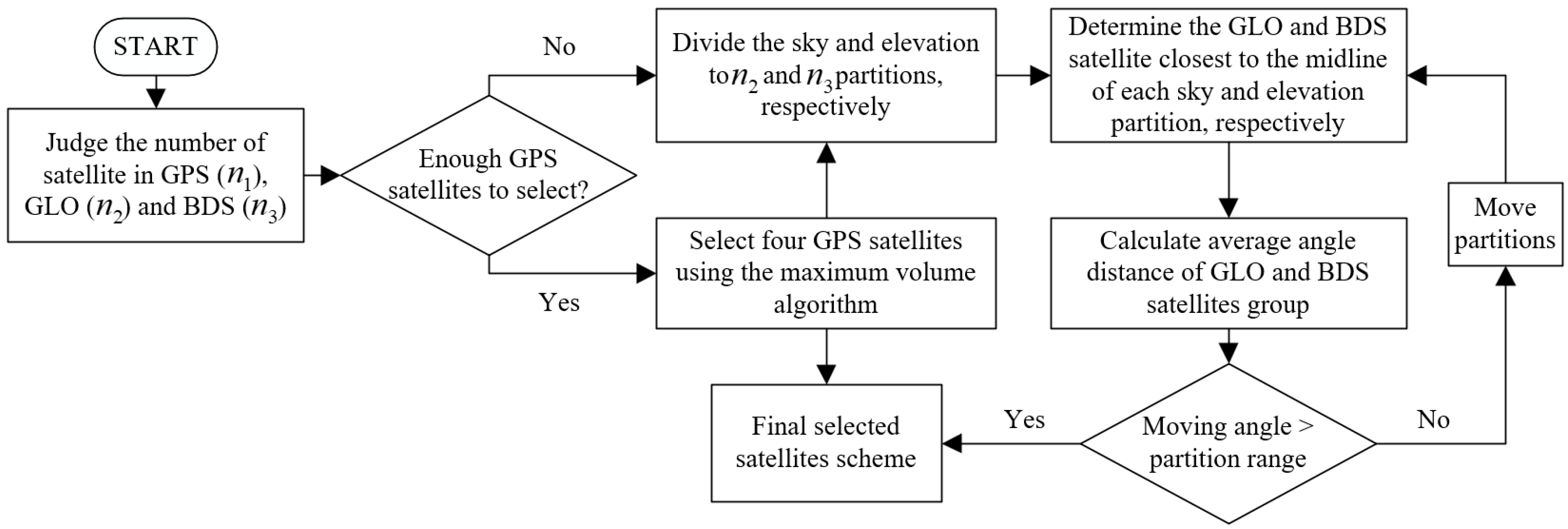
3.1. The Combination of Three Different Satellite Selection Algorithms

To reduce the excessive redundant information and guarantee similar positioning accuracy with an original solution in GPS/BDS/GLONASS kinematic PPP, an appropriate satellite selection model which can adapt PPP technique should be proposed. However, although GNSS constellations have similar capabilities, the satellite type, geometric spatial structure, and communication mode of each constellation are not necessarily the same. For instance, GPS and GLONASS are composed of MEO satellites while BDS includes GEO, MEO, and IGSO satellites. Due to different characteristics of GNSS, a single satellite selection algorithm sometimes seems to not be suitable when it comes to GPS/BDS/GLONASS satellites. Thus, to reduce the computational load of the GNSS equipment and obtain appropriate accuracy and reliability in GPS/BDS/GLONASS kinematic PPP, we propose the NSS model that includes three different satellite selection algorithms: the maximum volume algorithm, the fast-rotating partition satellite selection algorithm, and the elevation partition satellite selection algorithm.

In the process of establishing the NSS model, the accuracy and characteristics of different constellations and satellite selection algorithms were all considered. As the first and well-known GNSS system that has been fully operational, GPS has better positioning accuracy and reliability when BDS and GLONASS are compared. Thus, to ensure the positioning accuracy of the NSS model, the maximum volume algorithm is applied in the GPS satellites because GDOP is inversely proportional to the volume and better GDOP can partly reflect the theoretical impact of the observational geometry. For the BDS and GLONASS satellites, they both have rather good coverage almost worldwide. Thus, we used two satellite selection algorithms (based on azimuth and elevation, respectively) in BDS and GLONASS to avoid the situation that excessive satellites are selected at some epochs if one algorithm is used. In this study, the fast-rotating partition satellite selection algorithm based on equal distribution of sky was adopted for the GLONASS satellites, which can greatly reduce the computation time when compared to the optimal DOP algorithm. Like the fast-rotating partition satellite selection algorithm, the elevation partition satellite selection algorithm is based on equal distribution of elevation. Additionally, we applied the elevation partition satellite selection algorithm in BDS. These three different selection algorithms formed the NSS model. It is succinct and fast because the huge amount of computation is reduced in the process of satellite selection. In addition, the considered characteristics of multi-GNSS can provide some assurance for the positioning accuracy. The flowchart of satellite selection is shown in Figure 3.

3.2. The Inheritance of Ambiguity

With the satellite selection algorithm, the possible problems should also be considered in its application in kinematic PPP. Due to satellite movement and the application of the satellite selection algorithm, it is common that satellites selected in different epochs are not all the same. One satellite selected in the previous epoch may not be selected in the next epoch. This will lead to a circumstance that the positioning process is based on discontinuous observations although the satellite is continuously observed. At this time, if we apply the satellite selection in SPP, there are no problems in the data process because SPP only uses pseudorange observations for positioning. However, when it comes to the kinematic PPP solution, the positioning will be affected by the constantly re-estimated ambiguity because of the application of phase observations. The satellite selection algorithm will cause a poor accuracy and reliability in kinematic PPP. Thus, a method that useful ambiguity information is inherited in the data process is proposed. In the process of this method, only the ambiguity of each satellite at the previous and the next epoch are kept. It is a simple storage operation and its computational costs can be ignored when the reduced computation in the satellite selection algorithm are compared. The main contents are as follows.

In the process of parameter estimation, the estimated values and variances of float ambiguity of all satellites are saved in a list which is continuously kept. Suppose the related information of satellite $s$ at epoch $a-1$ has been saved. From epoch $a$ to the epoch $m-1$, satellite $s$ is not selected but continuously observed. At epoch $m$, satellite $s$ is selected again. At this time, we add the previously estimated parameter and variance of ambiguity to the optimal estimation of the previous epoch. The method is not rigorous, but we can use it in actual situations. Taking the undifferenced and uncombined dual-frequency PPP model as an example. Satellite $s$ is selected at epoch $a-1$ and epoch $m$. In addition, it is continuously observed from epoch $a-1$ to epoch $m$ while the total number of visible satellites is $n$ at epoch $m-1$, then the transformation of the last best estimation (State matrix and Variance matrix) at epoch $m$ can be shown as follows. Equation (10) is the transformation of the best estimation for the state matrix. Equation (11) is the transformation of the best estimation for the variance matrix.

$$\begin{array}{l}{X}_{m-1}=[u,cd{\overline{t}}_r,{\mathrm{ZWD}}_r,\stackrel{\mathrm{Ionospheric}\mathrm{parameter}}{\overbrace{{\overline{I}}_{r,1}^1,\dots ,{\overline{I}}_{r,1}^{m-1}}},\underset{\mathrm{Ambiguity}\mathrm{on}{f}_1}{\underbrace{{\overline{N}}_{r,1}^1,\dots ,{\overline{N}}_{r,1}^{n-1}}},\stackrel{\mathrm{Ambiguity}\mathrm{on}{f}_2}{\overbrace{{\overline{N}}_{r,2}^1,\dots ,{\overline{N}}_{r,2}^{n-1}}}{]}_{1\times \left(3\mathrm{n}+2\right)}^{\mathrm{T}}\\ \to [u,cd{\overline{t}}_r,{\mathrm{ZWD}}_r,{\overline{I}}_{r,1}^1,\dots ,{\overline{I}}_{r,1}^{m-1},{\overline{N}}_{r,1}^1,\dots ,{\overline{N}}_{r,1}^{n-1},{\overline{N}}_{r,2}^1,\dots ,{\overline{N}}_{r,2}^{n-1},{\overline{N}}_{r,1}^s,{\overline{N}}_{r,2}^s{]}_{1\times \left(3\mathrm{n}+4\right)}^{\mathrm{T}}\end{array}$$

(10)

$$Q_{m-1}=\left[\begin{array}{ccc}{({\sigma }_{\mathrm{X}}^2)}_{3\times 3}& & \\ & \ddots & \\ & & {({\sigma }_{\mathrm{N}}^2)}_{2n\times 2n}\end{array}\right]\to \left[\begin{array}{ccccc}{({\sigma }_{\mathrm{X}}^2)}_{3\times 3}& & & & \\ & \ddots & & & \\ & & {({\sigma }_{\mathrm{N}}^2)}_{2n\times 2n}& & \\ & & & {\sigma }_{N_{s,1}}^2& \\ & & & & {\sigma }_{N_{s,2}}^2\end{array}\right],$$

(11)

where $X_{m-1}$ is the best estimation for the state vector at epoch $m-1$; $Q_{m-1}$ is the best estimation for the variance vector at epoch $m-1$. $\sigma$ is the standard deviation of the estimated parameter.

4. Test and Analysis

4.1. Time Complexity of the NSS Model

As our aim was to reduce the computational complexity and guarantee similar positioning accuracy with original solution in GPS/BDS/GLONASS kinematic PPP, the performance of the NSS model and other satellite selection algorithms should be compared. The time complexity is an important indicator of measuring the complexity and the amount of computation in an algorithm. Although we can evaluate the time complexity of algorithms with the running time of the source program, it is not appropriate because of the huge workload and the programming effect. In this study, we used asymptotical algorithm analysis to calculate the time complexity of different satellite selection algorithms. Additionally, considering the final positioning accuracy of kinematic PPP after the application of the satellite selection algorithm, we chose the optimal DOP algorithm for comparison. The positioning accuracy will be compared in the next part. The number of basic operations in these two algorithms is both assumed to be same, which is represented as $n$. The number of cycles is the deciding factor in the size of time complexity. As mentioned earlier, it is obvious that the number of cycles in the optimal DOP algorithm, maximum volume algorithm, fast-rotating partition satellite selection algorithm, and elevation partition satellite selection algorithm is $C_N^{n_1}$, $C_N^4$, $360/N$, and $90/N$, respectively. Thus, the time complexity of the optimal DOP algorithm and the NSS model can be described clearly in Equation (12).

$$\begin{array}{l}T{(n)}_{OptimalDOP}=O(n^{C_N^m})\\ {T(n)}_{NSS}=O(n^{C_G^4}+\frac{360}{N}+\frac{90}{N})=O(n^{C_G^4})\end{array},$$

(12)

where $O(n)$ is asymptotic time complexity; $N$ denotes the total visible satellites and $G$ denotes the number of GPS satellites.

With the result in Equation (12), we can know that the NSS satellite selection model has a similar performance in time complexity when maximum volume algorithm is compared. Additionally, if the same number of satellites are selected, the NSS satellite selection model has a better time complexity than that of the optimal DOP algorithm.

4.2. Positioning Accuracy of the NSS Model

In order to test and validate the proposed NSS model, the performance of dual-frequency GPS/BDS/GLONASS undifferenced and uncombined kinematic PPP using this satellite selection model was evaluated based on MGEX daily observations and measured GNSS data. The MGEX data collected on 27 August 2017 at five MGEX stations (DARW, GMSD, KARR, MRO1, and XMIS) were used to simulate the kinematic environment in this study. The measured GNSS data was collected on 23 January 2018 using a Trimble netR9 receiver in Wuhan University of Technology of Wuhan, Hubei province. The sampling frequency of the static data is 1 Hz and continued for 7 h. To evaluate the positioning accuracy of kinematic PPP with the NSS model, the result of the original PPP without the satellite selection algorithm and kinematic PPP with the optimal DOP algorithm (number of selected satellites: 12) were also used for comparison. For the processing strategy, all the PPP experiments were performed based on the opensource GAMP software which can be freely accessed through the GPS Toolbox webpage (i.e., https://www.ngs.noaa.gov/gps-toolbox/GAMP.htm) [31]. The precise products from Wuhan University were used and we estimated a receiver clock offset for one system and the inter-system bias parameter [32]. The carrier phase ambiguities were kept floating and estimated as constant for each continuous satellite arc. Additionally, the inheritance of ambiguity method was adopted. The weighing between the three systems was 1:1:1 in the software. Due to the worse orbit and clock quality of BDS GEO satellites [33,34], the weighing between the BDS GEO satellite and the other BDS satellite was 1:10 [35]. The related GDOP calculation also agrees with this weighing strategy.

4.2.1. The MGEX Data

In this study, the daily undifferenced and uncombined observations from five MGEX stations on DOY 239 in 2017 were processed in the kinematic PPP solution to simulate a kinematic environment. The IGS weekly solutions in Solution Independent Exchange (SINEX) format were adopted as the external reference coordinates. As an important indicator of theoretical impact of the observational geometry, the GDOP value of three PPP solutions should be analyzed. For brevity, only the results from the DARW station are presented. Figure 4 is the visible satellites using the original PPP (Left), NSS model (middle), and Optimal DOP algorithm (Right) at the last second. The daily satellite numbers of the NSS model and Optimal DOP algorithm for GPS, GLONASS, and BDS are shown in Figure 5, Figure 6 and Figure 7, respectively. Due to different satellite selection strategies of the NSS model (Volume, Azimuth, Elevation mask angle) and Optimal DOP algorithm (GODP), the daily selected satellites are not same. Figure 8 shows the time-dependent change of satellite number and GDOP. In Figure 8, the average satellite number of the original PPP model, NSS model, and optimal model is 26, 12, and 12, respectively. If the satellite selection algorithm is not used in the process of PPP, the GDOP less than 1.5 accounts for 100% and the average GDOP value is 1.07. If the proposed NSS model is used to select satellites, the GDOP less than 2.5 accounts for 98.7%, the GDOP less than 2.0 accounts for 88.4%, and the GDOP less than 1.5 accounts for 19.1%. The average GDOP value is 1.72. Moreover, the GDOP of the optimal DOP algorithm is statistically analyzed. The GDOP value less than 2.0 accounts for 99.7%, and the GDOP less than 1.5 accounts for 75.0%. The average GDOP value is 1.43. From the above analysis of the results, it can be seen that the original PPP has the best GDOP average value and the most visible satellites. The number of satellites in the NSS model solution is greatly reduced when the average values of satellite number and GDOP are compared with other solutions.

Figure 9 shows the position residuals of GPS/BDS/GLONASS kinematic PPP with undifferenced and uncombined observations in the East (E), North (N), and Up (U) directions. In Figure 9, it can be seen that the position residuals of the NSS model and the optimal DOP algorithm are similar, while the original PPP has a better accuracy at most of epochs, as the original PPP solution uses all visible satellites. To obtain the accurate position accuracy of kinematic PPP, we calculated the RMS of the position residuals based on the results after 10 min convergence. It can be known that the RMS of the position residuals of original PPP was 2.8 cm in the E direction, 1.1 cm in the N direction, and 1.9 cm in the U direction. The RMS of the position residuals was 2.9 cm in the E direction, 2.1 cm in the N direction, and 6.9 cm in the U direction with the NSS model. For the optimal DOP algorithm, the RMS of the position residuals was 6.3 cm in the E direction, 5.6 cm in the N direction, and 2.3 cm in the U direction. Thus, the RMS of the position error ($\sqrt{△e^2+△n^2+△u^2}$) is 3.6, 7.8, and 8.6 cm for the original solution, NSS model, and optimal DOP algorithm, respectively. It is clear that the GPS/BDS/GLONASS kinematic PPP with NSS model has a centimeter-level accuracy when the simulated kinematic data at the MGEX stations is used.

Table 2. The average percentages of the number of selected satellites with respect to all visible satellites.

	DARW	GMSD	KARR	MRO1	XMIS	Mean
Original PPP	100%	100%	100%	100%	100%	100%
NSS model	46.0%	48.3%	45.0%	45.4%	43.0%	45.5%
Optimal DOP	45.8%	51.1%	45.4%	46.8%	43.9%	46.6%

shows the average percentages of the number of selected satellites with respect to all visible satellites at five MGEX stations on DOY 239, 2017. It can be known that about 45.5% and 46.6% visible satellites will be selected in NSS model and optimal DOP method, respectively.

Table 3. The RMSs of position errors at five MGEX stations (cm).

	DARW	GMSD	KARR	MRO1	XMIS	Mean
Original PPP	3.6	2.7	2.9	3.1	2.8	3.0
NSS model	7.8	8.7	6.4	8.7	7.2	7.8
Optimal DOP	8.6	5.3	8.3	6.2	8.1	7.3

is the RMSs of position errors at five MGEX stations. The position accuracy of original solution, NSS model, and optimal DOP algorithm is 3.0, 7.8, and 7.3 cm, respectively. Compared with the original solution, more than half of the satellites are removed in the NSS model. Additionally, the NSS model has similar position accuracy with the optimal DOP method.

Table 4. The computing time of daily data processing using the original PPP and NSS model, respectively (s).

	Original PPP	NSS Model	Improved
DARW	130.440	62.823	51.8%
GMSD	78.570	45.342	42.3%
KARR	112.436	62.214	44.7%
MRO1	103.957	60.057	42.2%
XMIS	112.781	60.924	46.0%
Mean	107.637	58.272	45.9%

shows the computing time of daily data processing using the original PPP and NSS model, respectively. From Table 4, we can know that the mean computing time of the original PPP and NSS model is 107.637 and 58.272 s, respectively. About 45.9% is improved in computing time. Thus, the centimeter-level positioning error can be accepted when it comes to the GPS/BDS/GLONASS kinematic PPP. This is because the NSS model solution reduces the computational complexity and excessive redundant information greatly at the same time.

4.2.2. The Measured Data

In order to prove the reliability of the proposed algorithm in more detail, GPS/BDS/GLONASS undifferenced and uncombined kinematic PPP was realized with the measured data. In this experiment, the results of GPS PPP with ambiguity resolution at static model were used as a reference truth value. Figure 10 shows the satellite number and GDOP of different satellite selection solutions. In Figure 10, the average satellite number of the original PPP model, NSS model, and optimal model is 26, 12, and 12, respectively. The average percentages of the number of selected satellites with respect to all visible satellites for the NSS model and optimal model is 46.2% and 46.8%. It means that less than half of the visible satellites are selected and the NSS model has the same average satellite number with the optimal model. For GDOP, the average values of the original PPP, NSS model, and optimal DOP algorithm are 1.16, 1.74, and 1.47, respectively. The NSS model fully meets the requirements for general kinematic positioning, such that the satellite GDOP of the position should be less than five [19].

To obtain the accurate position accuracy of kinematic PPP, we also calculated the RMS of the position residuals based on the results after 10 min convergence in Figure 11. It can be calculated that the RMS of the position residuals of original PPP was 1.6 cm in the E direction, 1.7 cm in the N direction, and 4.2 cm in the U direction. Additionally, the RMS of the position residuals was 8.1 cm in the E direction, 2.3 cm in the N direction, and 6.5 cm in the U direction with the NSS model. For the optimal DOP algorithm, the RMS of the position residuals was 4.5 cm in the E direction, 4.3 cm in the N direction, and 7.6 cm in the U direction. Thus, the RMS of the position error is 4.8, 10.6, and 9.8 cm for the original solution, NSS model, and optimal DOP algorithm, respectively. Due to the influence of multipath and cycle slips, the positioning accuracy of the measured data is not as good as that of the MGEX data. However, we can know that the GPS/BDS/GLONASS kinematic PPP with the NSS model has a similar accuracy to the optimal DOP algorithm solution when it is used in practical application. Additionally, the computing time of data processing using the original PPP and NSS model solution is 873.007 and 509.938 s, respectively. Thus, it is beneficial to the application of PPP in low-cost GNSS receivers because the NSS model has better performance on the computational complexity and redundant information.

The above results mean that the computational load could be significantly reduced in undifferenced and uncombined GPS/BDS/GLONASS kinematic PPP with the use of the proposed NSS model. Additionally, the positioning accuracy of the NSS model PPP solution is still within the requirement and similar to the optimal DOP algorithm solution. This study can provide a reference for the application of satellite selection algorithms in real-time kinematic PPP in low-cost GNSS receivers.

5. Conclusions

PPP can be widely used in many fields to provide spatial and temporal information due to its high accuracy and reliability. However, with the development of GNSS constellations, the increasing visible satellites also bring a huge computation load to the GNSS equipment in a kinematic environment. Thus, computational complexity and excessive redundant information should be considered in real-time kinematic PPP. At this time, the satellite selection algorithm that can effectively reduce the computational complexity and guarantee centimeter-level positioning accuracy with original solution causes us to consider its application in kinematic PPP.

Based on the characteristics of different satellite selection algorithms and GNSS constellations, we proposed a new satellite selection approach for GPS/BDS/GLONASS kinematic PPP with undifferenced and uncombined observations. The constantly re-estimated ambiguity encountered in the application of satellite selection algorithm was also considered with the method that is the inheritance of ambiguity. This NSS model includes three different algorithms (maximum volume algorithm, fast-rotating partition satellite selection algorithm, and the elevation partition satellite selection algorithm), and these algorithms were applied in GPS, GLONASS, and BDS, respectively. The principle of this classification is mainly decided by the accuracy and spatial distribution of these three constellations. The characteristics of different satellite selection algorithms was also considered. Compared with the optimal DOP algorithm, a huge amount of computation is reduced in the NSS model due to the conciseness of satellite selection algorithms and the structure of system classification. In order to verify the positioning accuracy of the NSS model, the original PPP with all visible satellites and optimal DOP algorithm was compared based on the MGEX data and the measured data. Results show that the number of visible satellites was reduced greatly, and a centimeter-level positioning accuracy can be obtained with the NSS model in GPS/BDS/GLONASS kinematic PPP while the original PPP and optimal DOP algorithm PPP solutions were compared.

In general, this study provided a new satellite selection approach to reduce the computational complexity and excessive redundant information in GPS/BDS/GLONASS kinematic PPP. In addition, it proposed a method to solve the situation of constantly re-estimated integer ambiguity in PPP when the satellite selection algorithm is used. In the future, for the reduction of the amount of computation and better real-time performance, the application of the satellite selection algorithm that considers satellite quality for kinematic PPP with fixed integer ambiguity may attract more attention.

References

1. Alkan, R.M.; Saka, M.H.; Ozulu, İ.M.; İlçi, V. Kinematic Precise Point Positioning Using GPS and Glonass Measurements in Marine Environments. Measurement 2017, 109, 36–43. [Google Scholar] [CrossRef]
2. Kouba, J.; Héroux, P. Precise Point Positioning Using IGS Orbit and Clock Products. GPS Solut. 2001, 5, 12–28. [Google Scholar] [CrossRef]
3. Zumberge, J.F.; Heflin, M.B.; Jefferson, D.C.; Watkins, M.M.; Webb, F.H. Precise point positioning for the efficient and robust analysis of GPS data from large networks. J. Geophys. Res. Solid Earth 1997, 102, 5005–5017. [Google Scholar] [CrossRef] [Green Version]
4. Wang, L.; Li, Z.; Ge, M.; Neitzel, F.; Wang, Z.; Yuan, H. Validation and Assessment of Multi-GNSS Real-Time Precise Point Positioning in Simulated Kinematic Mode Using IGS Real-Time Service. Remote Sens. 2018, 10, 337. [Google Scholar] [CrossRef] [Green Version]
5. Jiao, G.Q.; Song, S.L.; Ge, Y.L.; Su, K.; Liu, Y.Y. Assessment of BeiDou-3 and Multi-GNSS Precise Point Positioning Performance. Sensors 2019, 19, 2496. [Google Scholar] [CrossRef] [Green Version]
6. Yasyukevich, Y.; Astafyeva, E.; Padokhin, A.; Ivanova, V.; Syrovatskii, S.; Podlesnyi, A. The 6 September 2017 X-Class Solar Flares and Their Impacts on the Ionosphere, GNSS, and HF Radio Wave Propagation. Space Weather Int. J. Res. Appl. 2018, 16, 1013–1027. [Google Scholar] [CrossRef]
7. Jacobsen, K.S.; Andalsvik, Y.L. Overview of the 2015 St. Patrick’s day storm and its consequences for RTK and PPP positioning in Norway. J. Space Weather Space Clim. 2016, 6. [Google Scholar] [CrossRef]
8. RISDE. Global Navigation Satellite System GLONASS—Interface Control Document, Version 5.1; Russian Institute of Space Device Engineering: Moscow, Russia, 2008. [Google Scholar]
9. EU. European GNSS (Galileo) Open Service Signal in Space Interface Control Document; European Union: Brussels, Belgium, 2014. [Google Scholar]
10. CSNO. BeiDou Navigation Satellite System Signal in Space Interface Control Document: Open Service Signal (Version 2.0); China Satellite Navigation Office: Beijing, China, 2013. [Google Scholar]
11. CSNO. Report on the Development of BeiDou Navigation Satellite System (Version 2.2); China Satellite Navigation Office: Beijing, China, 2013. [Google Scholar]
12. Alcay, S.; Yigit, C.O. Network based performance of GPS-only and combined GPS/GLONASS positioning under different sky view conditions. Acta Geod. Geophys. 2017, 52, 345–356. [Google Scholar] [CrossRef]
13. Nie, Z.; Gao, Y.; Wang, Z.; Ji, S. A new method for satellite selection with controllable weighted PDOP threshold. Surv. Rev. 2016, 49, 285–293. [Google Scholar] [CrossRef]
14. Kihara, M.; Okada, T. A Satellite Selection Method and Accuracy for the Global Positioning System. Navigation 1984, 31, 8–20. [Google Scholar] [CrossRef]
15. Swaszek, P.F.; Hartnett, R.J.; Seals, K.C. Multi-Constellation GNSS: New Bounds on DOP and a Related Satellite Selection Process. In Proceedings of the 29th International Technical Meeting of the Satellite Division of the Institute of Navigation, Portland, OR, USA, 12–16 September 2016; pp. 228–235. [Google Scholar]
16. Meng, F.; Wang, S.; Zhu, B. Research of Fast Satellite Selection Algorithm for Multi-constellation. Chin. J. Electron. 2016, 25, 1172–1178. [Google Scholar] [CrossRef]
17. Blanco-Delgado, N.; Nunes, F.D. Satellite Selection Method for Multi-Constellation GNSS Using Convex Geometry. IEEE Trans. Veh. Technol. 2010, 59, 4289–4297. [Google Scholar] [CrossRef]
18. Roongpiboonsopit, D.; Karimi, H.A. A Multi-Constellations Satellite Selection Algorithm for Integrated Global Navigation Satellite Systems. J. Intell. Transp. Syst. 2009, 13, 127–141. [Google Scholar] [CrossRef]
19. Li, F.; Li, Z.; Gao, J.; Yao, Y. A Fast Rotating Partition Satellite Selection Algorithm Based on Equal Distribution of Sky. J. Navig. 2019, 72, 1053–1069. [Google Scholar] [CrossRef]
20. Gao, X.; Dai, W.; Song, Z.; Cai, C. Reference satellite selection method for GNSS high-precision relative positioning. Geod. Geodyn. 2017, 8, 125–129. [Google Scholar] [CrossRef] [Green Version]
21. Huang, P.P.; Rizos, C.; Roberts, C. Satellite selection with an end-to-end deep learning network. GPS Solut. 2018, 22, 108. [Google Scholar] [CrossRef]
22. Kaplan, E.D.; Hegarty, C.J. Understanding GPS: Principles and Applications, 2nd ed.; Artech House: Norwood, MA, USA, 2006. [Google Scholar]
23. Li, Z.K.; Chen, F. Improving availability and accuracy of GPS/BDS positioning using QZSS for single receiver. Acta Geod. Geophys. 2017, 52, 95–109. [Google Scholar] [CrossRef]
24. Montenbruck, O.; Steigenberger, P.; Prange, L.; Deng, Z.; Zhao, Q.; Perosanz, F.; Romero, I.; Noll, C.; Stuerze, A.; Weber, G.; et al. The Multi-GNSS Experiment (MGEX) of the International GNSS Service (IGS) —Achievements, prospects and challenges. Adv. Space Res. 2017, 59, 1671–1697. [Google Scholar] [CrossRef]
25. Zhou, F.; Dong, D.A.; Ge, M.R.; Li, P.; Wickert, J.; Schuh, H. Simultaneous estimation of GLONASS pseudorange inter-frequency biases in precise point positioning using undifferenced and uncombined observations. GPS Solut. 2018, 22. [Google Scholar] [CrossRef]
26. Schönemann, E.; Becker, M.; Springer, T. A new Approach for GNSS Analysis in a Multi-GNSS and Multi-Signal Environment. J. Geod. Sci. 2011, 1, 204–214. [Google Scholar] [CrossRef] [Green Version]
27. Odijk, D.; Zhang, B.C.; Khodabandeh, A.; Odolinski, R.; Teunissen, P.J.G. On the estimability of parameters in undifferenced, uncombined GNSS network and PPP-RTK user models by means of system theory. J. Geod. 2016, 90, 15–44. [Google Scholar] [CrossRef]
28. Yan, X.; Yang, G.; Shi, J.; Xu, C. Carrier phase-based ionospheric observables using PPP models. Geod. Geodyn. 2017, 8, 17–23. [Google Scholar]
29. Liu, T.; Yuan, Y.B.; Zhang, B.C.; Wang, N.B.; Tan, B.F.; Chen, Y.C. Multi-GNSS precise point positioning (MGPPP) using raw observations. J. Geod. 2017, 91, 253–268. [Google Scholar] [CrossRef]
30. Guo, F.; Zhang, X.H.; Wang, J.L.; Ren, X.D. Modeling and assessment of triple-frequency BDS precise point positioning. J. Geod. 2016, 90, 1223–1235. [Google Scholar] [CrossRef]
31. Zhou, F.; Dong, D.; Li, W.; Jiang, X.; Wickert, J.; Schuh, H. GAMP: An open-source software of multi-GNSS precise point positioning using undifferenced and uncombined observations. GPS Solut. 2018, 22, 33. [Google Scholar] [CrossRef]
32. Li, X.; Zus, F.; Lu, C.; Dick, G.; Ning, T.; Ge, M.; Wickert, J.; Schuh, H. Retrieving of atmospheric parameters from multi-GNSS in real time: Validation with water vapor radiometer and numerical weather model. J. Geophys. Res. Atmos. 2015, 120, 7189–7204. [Google Scholar] [CrossRef] [Green Version]
33. Kazmierski, K.; Sosnica, K.; Hadas, T. Quality assessment of multi-GNSS orbits and clocks for real-time precise point positioning. GPS Solut. 2017, 22, 11. [Google Scholar] [CrossRef] [Green Version]
34. Kazmierski, K.; Hadas, T.; Sosnica, K. Weighting of Multi-GNSS Observations in Real-Time Precise Point Positioning. Remote Sens. 2018, 10, 84. [Google Scholar] [CrossRef] [Green Version]
35. Li, P.; Zhang, X.; Guo, F. Ambiguity resolved precise point positioning with GPS and BeiDou. J. Geod. 2017, 91, 25–40. [Google Scholar] [CrossRef]
Figure 1. The fast-rotating partition satellite selection algorithm.
Applsci 09 05280 g001
Figure 2. The elevation partition satellite selection algorithm.
Applsci 09 05280 g002
Figure 3. Flowchart of the NSS model.
Applsci 09 05280 g003
Figure 4. The visible satellites using the original Precise Point Positioning (PPP) (Left), NSS model (middle), and Optimal dilution of precision (DOP) algorithm (Right) at the DARW station.
Applsci 09 05280 g004
Figure 5. The visible GPS satellite number using the NSS model (Left) and Optimal DOP algorithm. (Right) at the DARW station (day of year (DOY) 239, 2017).
Applsci 09 05280 g005
Figure 6. The visible GLONASS satellite number using the NSS model (Left) and Optimal DOP algorithm (Right) at the DARW station (DOY 239, 2017).
Applsci 09 05280 g006
Figure 7. The visible BDS satellite number using the NSS model (Left) and Optimal DOP algorithm (Right) at the DARW station (DOY 239, 2017).
Applsci 09 05280 g007
Figure 8. The satellite number and geometric position dilution of precision (GDOP) of kinematic PPP using the original PPP, NSS model, and Optimal DOP algorithm at the DARW station.
Applsci 09 05280 g008
Figure 9. Position residuals of PPP using different satellite selection solutions at DARW station.
Applsci 09 05280 g009
Figure 10. The satellite number and GDOP of kinematic PPP using the original PPP, NSS model, and Optimal DOP algorithm based on the measured data.
Applsci 09 05280 g010
Figure 11. Position residuals of PPP using different satellite selection solutions based on the measured data.
Applsci 09 05280 g011