Featured Application
The results of this article can be used for the precise control and positioning system of articulated vehicles.
Abstract
Owing to the harsh environment of underground mines, autonomous underground articulated vehicles (UAVs) with precise control and positioning system are particularly important. However, the ambiguity of steering characteristics hinders the development of UAVs. This study presents a model-based method to uncover the steering characteristics of a UAV. Firstly, a hybrid model of UAV was established, which included a dynamic model of articulated frames and a model of the hydraulic power steering system. Secondly, a field test of a typical UAV, a load-haul-dump (LHD) with 4 m3 capacity, was carried out. In order to verify the correctness of the established model and the accuracy of the involved parameters, the field test results were used to verify the dynamic model in time and frequency domains. Then, the steering characteristics of the UAV were uncovered based on the verified hybrid model, and the results showed that the increased load would increase ‘oversteering’ under the same articulation angle and that the error of trajectory exceeded 0.3 m. In addition, the deviations of trajectories between the two frames were revealed during the transient steering process, and the maximum deviation reached 0.21 m when the velocity was 2 m/s and the articulation angle was 15°. The comprehensive results indicate that the steering characteristics of UAVs cannot be ignored in regard to precise autonomous control and positioning.
1. Introduction
With excellent maneuverability and efficiency, underground articulated vehicles (UAVs) are widely used in the processes of drilling, transportation, supporting and charging, which are of decisive significance to the production of underground mines [1,2,3]. The increasing depth of mines leads to significant local environment problems, such as high temperature and high humidity, which cause greater difficulty for mining, and potentially threaten the safety and health of the underground staff. Therefore, autonomous UAVs are urgently needed. Because of the specialty of steering, the lateral precise control of UAV is an important issue [4,5], which is usually based on the dynamic model and steering characteristics of the UAV. The steering characteristics reflect the control performance, and are the main means to evaluate the handling stability and path tracking of the vehicle [6,7,8]. However, the simplified models and ambiguous steering characteristics of UAVs hinder their precise control.
In recent years, much research has been directed towards the precise modeling and control of UAVs [9,10,11,12]. Horton [13] et al. established a steering model of UAVs based on the relationship of velocity, centroid and handling stability. The simulation results showed that the velocity and centroid were the key parameters leading to oscillation and instability. Azad [14,15] et al. established a simplified three degree of freedom (DOF) model to analyze the snaking motion of UAVs and studied the relationship between lateral stability and steering characteristics. Pazooki [16] et al. established a kinematic model on the basis of a dynamic model, and the steady steering and pulse steering processes were analyzed. Nayl [17,18] et al. studied the effect of kinematic parameters on a motion planning system, and the kinematic model was used during the process of modeling and control. Gao [4] et al. established a 12 DOF dynamic model of UAV and uncovered the instability area considering the influence of bulk modulus of hydraulic oil. Based on the instability results, an Ackman-based hierarchical controller was designed to improve the stability of UAVs. Bai [19,20] et al. designed a nonlinear model predictive controller based on the kinematic model of a UAV, with a maximum error of 0.14 m.
The above studies focused on the stability of UAVs, and different models have been established to analyze the influencing factors on the stability. In addition, strategies were also designed to control lateral motion or improve the accuracy of path following. These achievements greatly improve the stability and control accuracy of UAVs. However, some shortcomings remain to be addressed; for instance, dynamic models have been greatly simplified for the control and analysis of UAV, e.g., the hydraulic power steering system has been separated from the dynamic model of the frames or even ignored. The involved kinematic model in control strategies has generally been based on steady steering, while the transient process and steering characteristics were ignored. Moreover, the trajectories of the front and rear frames were considered to be the same during the system of path following. In reality, the trajectories are different in the transient process of steering, and the process would also be different under different working conditions. Motivated by these shortcomings, we attempt to analyze the steering characteristics based on a hybrid model to uncover the relationship between dynamic steering and the response of frames. Several contributions are summarized as:
- (1)
- A hybrid model including a dynamic model of articulated frames and a model of a hydraulic power steering system is established.
- (2)
- A field test is carried out to verify the dynamic model in time and frequency domains.
- (3)
- The steering characteristics of a UAV, which involves the effects of load and velocity, are revealed based on the verified model.
The paper is organized as follows: In Section 2, the dynamic model of a UAV including the model of frames and steering system is presented. Section 3 is devoted to the verification of the dynamic model in time and frequency domains, and the field test setup is also presented. Section 4 analyzes the steering characteristics based on the established model and discuss the results. The conclusion is presented in the final section.
2. Dynamic Model of UAVs
UAVs are composed of front and rear frames, which are connected by a central articulated point. Steering motion is achieved by the change of articulation angle, which is driven by the hydraulic power steering cylinder. Therefore, dynamic models of UAVs are composed of a model of vehicle dynamics and a model of the hydraulic steering system.
2.1. Dynamic Model of Vehicle Frames
A diagram of UAV motion is shown in Figure 1; the motion can be described in the two sets of frames: the ISO (the longitudinal forward direction of vehicle is defined as X axis, vertical downward direction is defined as Z axis, Y axis is in right-hand coordinate system) front frame (X1Y1Z1) and ISO rear frame (X2Y2Z2). In addition, the detailed force information at the articulated point is also shown in Figure 1.
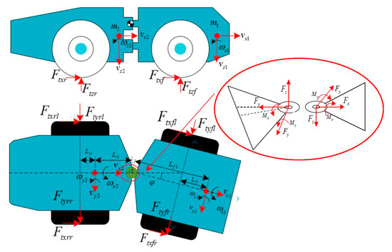
Figure 1.
Diagram of underground articulated vehicle (UAV) motion.
According to the relationship of the involved forces and moments shown in Figure 1, the motions of the UAV in the XOY plane (the lateral and longitudinal directions) are focused [10]. Based on Newton’s law, the dynamic model of UAV frames in different directions can be expressed as:
where the indexes 1 and 2 denote front and rear frames, respectively; ϕ is the articulation angle; m1 and m2 are the mass of front and rear frames, respectively; Iz1 and Iz2 are the moment of inertia in the z direction, respectively; Fx, Fy, and Mz are internal forces and moment at the central point; Fsxf, Fsyf, Fsxr, Fsyr, Mzf and Mzr are the forces and moments brought by the steering cylinder; and Ftxf, Ftyf, Ftxr, Ftyr, Mtzf, and Mtzr denote the front and rear tire forces and moments in the different x, y, and z directions, which can be expressed as:
where Lf1 and Lr1 are the distance between the mass centers of the front and rear frames and corresponding axle, respectively; and B is half of the wheel track.
In addition, the longitudinal and lateral tire force can be given by the Magic Formula [21]:
where Xm denotes the sideslip angle or slip ratio of the tire; Fm denotes the lateral or longitudinal force of tire; the parameters Sx, Sy, B, C, D, and E are constant, where in this study Sx = 0, Sy = 0, and other parameters are calculated by equations with vertical load.
The slip ratio of different tires can be described as:
where rdij denotes the rolling radius of different tires, ωij denotes the angular velocity of different tires, and vxij denotes the longitudinal velocity of front and rear frame, which can be written as:
The sideslip angle of different tires can be described as:
According to the kinematic constraints of the central articulation point, the constraints of the linear velocity in different directions can be given by:
where Lf2 and Lr2 are the distances between the mass centers of front and rear frames and the central articulation point, respectively.
We substitute Equations (3)–(8) into Equations (1) and (2) to obtain the dynamic model of frames, while the forces and moment originating from the hydraulic steering system are not given. Therefore, the model of the hydraulic steering system will be established to obtain the related forces and moments.
2.2. Model of Hydraulic Steering System
The hydraulic steering system of the UAV is shown in Figure 2. The rodless cavity of the left cylinder is connected with the rod cavity of the right cylinder, and the main directional valve, which is from the M4 series of Bosch Rexroth, determines the direction of oil under pressure, which drives the extension and retraction of the cylinder to steer.
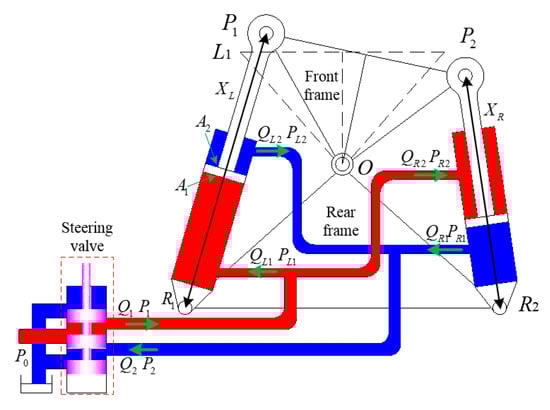
Figure 2.
Hydraulic steering system of UAV.
It should be emphasized that the steering valve has a pressure compensation in front of the spool, which can ensure a constant pressure difference between the inlet pressure and load pressure. Therefore, the input flow of the system is only related to the open area of the spool, which is determined by the control current of spool. Then the input and output flow can be described as [22]:
where Iin denotes the control current, Cd denotes the flow coefficient, and A0 is the area of the orifice, which is related to the control current. P2, and P0 are the pressure of the return oil and atmosphere, respectively; ρ is the density of hydraulic oil; and Qin, Qout are the input and output flow of the system. The relationship of the control current and the input flow is shown in Figure 3, which is obtained from experiment data of the steering valve company, i.e., Bosch Rexroth.
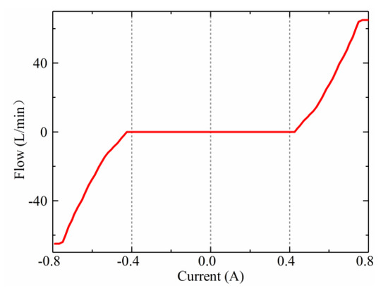
Figure 3.
Relationship of control current and input flow.
As shown in Figure 3, the positive current corresponds to the positive flow, which means the flow is led into the rodless cavity of the left cylinder to steer towards the right; conversely, negative current and flow means the flow is led into the right cylinder to steer towards the left. In addition, there are dead zones at −0.43 to 0.43 A, −0.77 to −0.80 A, and 0.77 to 0.80 A, where the flow shows obvious nonlinear characteristics, which originate from the friction, dead zone, etc., between the valve spool and sleeve. There is a linear relationship during other intervals, and the maximum flow is 68 L/min. According to Figure 3, the input and output flows of the system contain two parts, respectively, and the relationship can be described as:
where Q ij (i = L, R; j = 1, 2) denotes the flow of the rodless and rod cavities of the left and right cylinders, which can be expressed as:
where A1 and A2 are the action areas of the rodless and rod cavities, respectively; XR and XL are the displacements of right and left cylinders, respectively; V ij (i = L, R; j = 1, 2) denotes the volume of the rodless and rod cavities of left and right cylinders, respectively; K is the bulk modulus of hydraulic oil; and Cip denotes the coefficient of internal leakage. Pij (i = L, R; j = 1, 2) denotes the pressure of the rodless and rod cavities of the left and right cylinders, respectively, and can be described as:
The force balance equation of steering cylinders can be expressed as [22]:
where fs is the coefficient of dynamic friction.
In addition to the above relationship of flow and force, there is also a kinematic relationship between the frames and steering cylinders [10], as illustrated in Figure 4. The angles between two cylinders and frames are represented by γ and β, respectively.
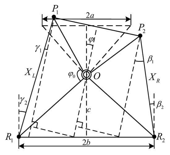
Figure 4.
Kinematic relationship of steer cylinder and frames.
According to the relationship in Figure 4, the displacement of the two cylinders can be expressed as:
In addition, the angles of cylinders and frames are related to the articulation angle, which can be described as:
Based on the sine theorem, the angle of cylinders and front frame can be described as:
where
Combining Equations (14)–(17), the forces and moments brought about by the steering cylinder can be expressed as:
Based on the derivation above, we obtain the hybrid model of the UAV, which includes the dynamic model of frames (i.e., Equations (1) and (2)) and the model of the hydraulic steering system (i.e., Equation (18)). The relationship between the models is shown in Figure 5. Notably, neither the throttle for longitudinal control nor the model of the power source were considered, since the model is verified under constant velocity conditions. However, the power system is also included in Figure 5, which involves the power of the hydraulic steering system and the driving force of vehicle.
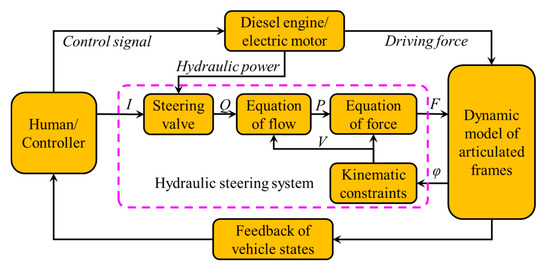
Figure 5.
Hybrid model relationship of hydraulic steering system and frames.
3. Validation of Dynamic Model
3.1. Field Test Setup
The field test UAV was a remote control (load-haul-dump vehicle; LHD) with a capacity of 4 m3 in; the test system is shown in Figure 6. All the sensors and modules were commercial products, and we only designed the installation frameworks. A serial port was used to connect with the remote control to record the signal of driving and steering, which was used as the input of the simulation model. An LMS SCADAS (①, SCM05) was used to record the data during the field test, and the sampling frequency was set as 100 Hz [23]. Two inertial measurement units (IMUs) (②, ③, SC-AHRS-200A) were installed in the front and rear frames, respectively. Two kinds of encoders were used to measure the articulated angle of the frame (④, MIRAN WOA-C) and the speed of transmission (⑤, SCHMEASAL IFL 5-18M-10P), respectively. A gyroscope (⑥, Beiwei) with high precision was installed to provide the reference values. In addition, two pressure sensors (⑦, AE-H) were installed near the rodless and rod cavities of left cylinder, and two displacement sensors (⑧, WFS-1000-P15-11R5) were installed at the two steering cylinders, respectively.
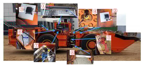
Figure 6.
The system configuration of the field test.
Usually, characteristics of the route for an LHD are special in underground mines, and always include a square turn and change of operation direction. Thus, the route of the field test was planned as shown in Figure 7, where the direction of the arrow represents the direction of the LHD and the solid and hollow lines correspond to the forward and backward directions, respectively. The key dimensions were L1 = 50 m, L2 = 20 m. The road of the whole field test site was uneven, and the uncertainty of the road surface would have made it difficult to verify the model during the whole test process, therefore, we intercepted a piece of typical test data in which the speed of vehicle was constant and the road was relatively flat to verify the model.
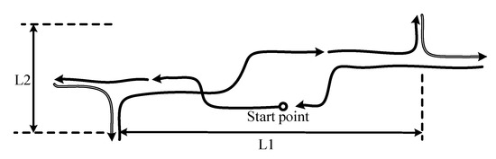
Figure 7.
Route of field test.
3.2. Discussion of Field Test Results
In order to verify the dynamic model, the results of simulation and field test were compared, and the simulation carried out by MATLAB/Simulink. A region with constant longitudinal velocity and different steering maneuvers was selected for analysis in which the velocity was 3.1 km/h. In addition, the simulation input signal of steering was also the same as the signal in the field test, which is shown in Figure 8. According to the steering signal in Figure 8, steering maneuvers with different amplitudes in left and right directions are included, which can cover the different actual operating conditions.
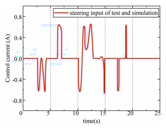
Figure 8.
Steering signal of test and simulation.
It should be noted that the error of the steering system is always obtained by constant radius steering (0–360 degree), i.e., stable steering, while the experiment was not processed considering the limitations of the field test site. For the field test conditions in this article, different amplitudes and directions were considered that can represent the dynamic characteristics of the hydraulic steering system. The dynamic characteristics of the steering system are particularly important during the dynamic driving process, therefore, we used the consistent dynamic response results to verify the dynamic model.
As the most important information of UAVs, the articulation angle was considered first, and the comparison results are shown in Figure 9. According to the comparison results in Figure 9, the response of the articulation angle for the simulation model and test vehicle is the same under different steering maneuvers, including the process and end of steering. Not only is the steering angle during the steering process the same, but also the final steering angle was the same. The Root Mean Square (RMS) of the error is 0.1 degree. In addition, the detailed information shows that some ripples occurred in the field test. Similarly, the simulation results have the same characteristics.
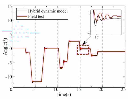
Figure 9.
Comparing results of articulation angle.
The comparison results of the two steering cylinders’ displacements are shown in Figure 10. The result of the simulation is the same as the field test results, except for some errors after steering. The maximum error during the comparison region is 0.01 m. The accuracy is high enough to simulate the steering response considering the errors brought about by the installation of sensors.
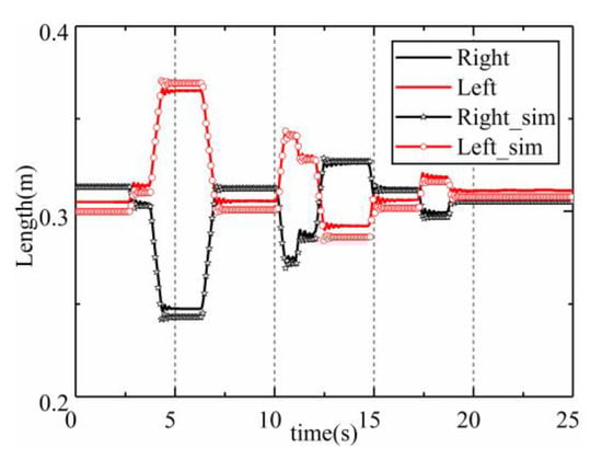
Figure 10.
Comparing results of displacements of steering cylinders.
The results of steering cylinder pressure are shown in Figure 11. During the start stage (0–2.5 s), the pressure is 3 MPa in the field test, but the simulation pressure is the atmosphere pressure of 0.1 MPa. This is because the stage is only the start of the simulation and there is no load in the steering system according to the results in Figure 11a,b. The pressure peak values of the simulation and field test appear at the same time around 15 s and the approximate value is 14 MPa. In addition, the trends and values of pressure are almost identical according to the detailed comparison results in Figure 11c. Firstly, the trends are the same during the steering process. However, the trends are obviously different after steering. The test results show that the pressure fluctuates repeatedly, and the attenuation is not obvious. Although simulation data show the same fluctuation, the attenuation is faster. In addition to the above differences, the system average pressure is almost the same after the fluctuation. As is well known, the attenuation of vibration is directly related to the damping of the system. According to the above results, the main difference between the simulation model and target vehicle is the numerical difference of damping.
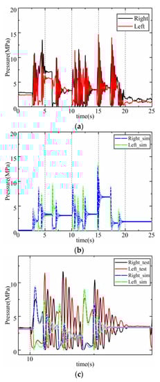
Figure 11.
Comparison results of steering pressure. (a) Field test results; (b) simulation results; (c) detailed comparison results.
The angular velocity of the yaw motions is compared with the corresponding simulation results, which are shown in Figure 12. As we can see from Figure 12a, the angular velocity trends of the front and rear frames in the test coincide with the simulation results, and the peak value and mean value are almost the same. However, the fluctuations are more obvious in the field test, which means that the oscillation occurred after the steering maneuvers, i.e., the snake motion. Although the same oscillation occurred in the simulation results, the amplitude and attenuation are different. Therefore, we verify the dynamic model in the frequency domain by comparing the frequency characteristic of the oscillation.
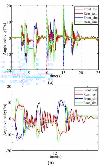
Figure 12.
Comparison results of angular velocity. (a) Results of test and simulation; (b) detailed comparison results.
Considering that the time of steering is short and the response data is a non-stationary signal, the short-time Fourier transform (SFT) is adopted. In addition, the frequency value of fluctuation is very small and the frequency results of the constant part in the signals would cover the corresponding results of fluctuation. Therefore, the baseline estimation and denoising with sparsity (BEADS) algorithm is adopted to remove the constant value in the signal. The data of the articulation angle is analyzed, and the corresponding results are shown in Figure 13. Due to the process of removal, there are other frequency components during the steering process according to Figure 13, while only the peak frequency (main frequency) is the focus of attention and verification. For test results in Figure 13a, the same peak frequency, 3.9 Hz, occurs after all steering maneuvers. The same frequency value occurs in the data of the yaw angle velocity and steering pressure (results not shown due to the similarity of comparison with the results of articulated vehicles), which means that the steering motion leads to the vibration of frames and the fluctuations in the hydraulic steering cylinders. In addition, the frequency of 50 Hz appears in the whole region, which is caused by the power frequency. Similarly, the same peak frequency occurs in a steady time period, although the amplitude varies greatly. These results indicate that the frequency of the fluctuation in field test is in good agreement with the simulation.
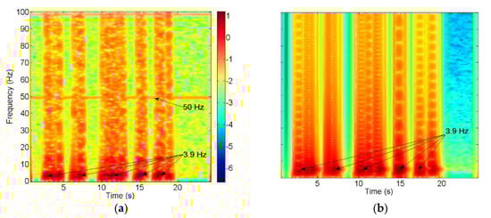
Figure 13.
Comparing frequency results of articulation angle by short-time Fourier transform (SFT). (a) SFT results of field test; (b) SFT results of simulation results.
Based on the above-verified results, we can conclude that the established dynamic model of the UAV is correct and accurate enough to simulate the dynamic response of the frames and hydraulic steering system, and that this model can be used as the basis for further analysis.
4. Analysis of Steering Characteristics
Owing to the mobility of the two frames, the different rotated angles of the frames cause changes of the steering center, as shown in Figure 14. Notably, these results are obtained by the verified dynamic model. For the situation in Figure 14a, the front frame rotates with a large angle when it comes to steer, and the center of rotation is lower than the articulation point. In contrast, the rear frame rotates with a large angle in Figure 14b, and the center of rotation is higher than the articulation point. The above situations are similar with oversteering and understeering situations, while it often appears as Figure 14c during normal working conditions. However, the quantitative relationship between the motion of the two frames is ambiguous. After the validation in the above sections, the dynamic model is used to analyze the steering characteristics of UAVs and determine the quantitative relationship, in which different load conditions are involved according to the working characteristics of the LHD, with the velocity set as 2 m/s. The angular velocity response results are shown in Figure 15. As we can see from Figure 15, when the load of the front frame increases, the peak angular velocity of the front frame decays; in contrast, the rear frame has an obvious rise. According to the results in Figure 16, the trajectories of the front frame at different loads are different, although the articulation angle is the same. Moreover, the maximum error exceeds 0.3 m in the lateral direction, which is greater than the accuracy of some control systems. Therefore, the increasing load of the front frame leads to a decrease in the corresponding angular velocity, which increases the ‘oversteer’. Thus, these characteristics should be involved in the control of UAVs.
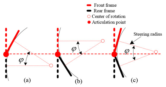
Figure 14.
Steering characteristic of UAVs. (a) Front frame rotates with larger scale; (b) rear frame rotates with larger scale; (c) two frames rotate with comparative scales.
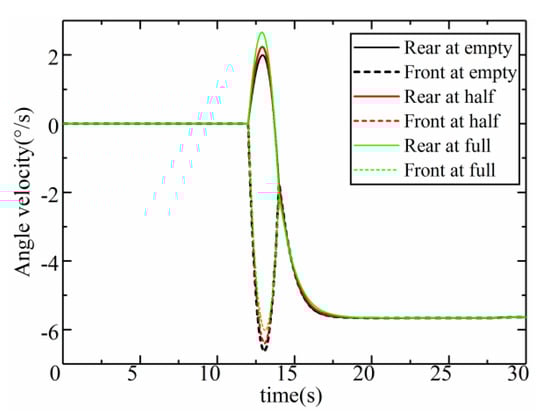
Figure 15.
Steering response of frames at different load conditions.
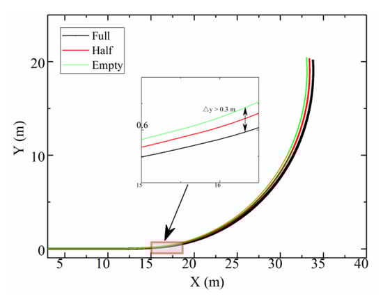
Figure 16.
Trajectories of front frame at different load conditions.
In many studies of autonomous UAVs, the front frame is selected as the representative motion and trajectory of the UAV. The motion and trajectory of the frames are the same according to the geometric characteristics when the vehicle goes through the process of steady steering (Figure 14), while the transient process of steering is ignored. Therefore, the validated model is used to analyze the difference between the two trajectories, in which the steady and transient processes are considered. The model-based analysis results of the two trajectories with a constant steering radius are shown in Figure 17, in which the velocity is set as the common velocity range in the longitudinal (x axis) direction (i.e., 2 m/s, 3 m/s, 4 m/s, respectively) and the articulation angle was set as 15 degrees under different velocity conditions.
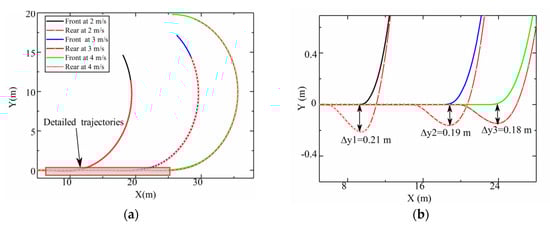
Figure 17.
Trajectory with constant steering radius at different velocity conditions. (a) Trajectories of frames at different velocities; (b) detailed information of trajectories under a transient steering process.
Indeed, the two trajectories coincide completely after the steering process according to Figure 17a, thus, it is reasonable to represent the vehicle by the front frame. However, it is worth noting that the rear frame trajectory deviates from the front frame according to the detailed information of trajectories in Figure 17b. The deviation occurs in the transient process of steering according to the time mark. The maximum error of the deviation is 0.21 m when the velocity is 2 m/s; this value is greater than the errors in some control and positioning systems used in UAVs [11,19]. The deviation decreases when the velocity increases. However, the errors are not negligible during the common velocity range according to the results shown in Figure 17b. Therefore, the deviation of the two frames cannot be neglected when it comes to the control, navigation, and positioning of autonomous UAVs.
5. Conclusions
In this paper, the steering characteristics of UAVs and the effects on trajectories were uncovered based on a validated hybrid dynamic model. Substantial results and contributions can be summarized as follows.
(1) A hybrid dynamic model of a UAV incorporating a dynamic model of frames and a hydraulic power steering system was established.
(2) A field test of a typical UAV, an LHD with 4 m3 capacity, was carried out. The results of articulation angle, and dynamic responses of frames and hydraulic steering system, were used to verify the hybrid model in the time domain. The relatively small errors in the time domain proved the validity of the established model. In addition, owing to the poor handling stability of the UAV, oscillation was found in the dynamic responses of the frames and hydraulic steering system. The results were used to verify the dynamic model, and the accuracy of the involved parameters in the dynamic model was checked by the frequency domain results obtained with SFT. The test and simulation results showed the same dominant frequency of 3.9 Hz simultaneously, proving the accuracy of the model and involved parameters.
(3) Based on the verified hybrid model, the steering characteristics of the UAV were uncovered, considering its load changes. The results showed that increasing the load of the front frame would lead to a decrease of the corresponding angular velocity, which would increase the ‘oversteer’. The trajectories’ deviation between empty and full load conditions in the lateral direction exceeded 0.3 m when the velocity was 2 m/s. Meanwhile, the effect of transient steering characteristics on the trajectories was investigated under different velocities. The maximum deviation of front and rear frame trajectories reached 0.21 m when the velocity was approximately 2 m/s.
(4) This hybrid dynamic model can be used to analyze the dynamic characteristics of UAVs and the hydraulic steering system. Although the focus of this paper is LHD, the established dynamic model can also be applied to different articulated vehicles, such as articulated drill jumbos, charging vehicles, mining dump trucks, tractors, and even some agriculture and forestry machinery. The steering characteristics mentioned above should be considered for precise control, navigation and positioning of UAVs, which is crucial for the above-mentioned articulated vehicles.
Author Contributions
L.G. and C.J. developed the dynamic model of UAV, L.G., Y.L., and C.J. processed the simulation and field test, L.G. wrote the article; F.M. and Z.F. supervised the overall study and field test and revised the article.
Funding
This research was funded the National Key Research and Development Program of China (Grant No. 2016YFC0802900), the National Natural Science Foundation of China (grant number 51774019) for the financial support.
Acknowledgments
The authors would like to acknowledge the Shandong Gold Group Co., Ltd. for the experimental UAV and sites.
Conflicts of Interest
The authors declare no conflict of interest. The funders had no role in the design of the study; in the collection, analyses, or interpretation of data; in the writing of the manuscript, or in the decision to publish the results.
References
- Li, J.; Zhan, K. Intelligent Mining Technology for an Underground Metal Mine Based on Unmanned Equipment. Engineering 2018, 3, 381–391. [Google Scholar] [CrossRef]
- Gustafson, A.; Paraszczak, J.; Tuleau, J.; Schunnesson, H. Impact of technical and operational factors on effectiveness of automatic load-haul-dump machines. Min. Technol. 2017, 4, 185–190. [Google Scholar]
- Yin, Y.; Rakheja, S.; Boileau, P. Multi-performance analyses and design optimisation of hydro-pneumatic suspension system for an articulated frame-steered vehicle. Veh. Syst. Dyn. 2019, 57, 108–133. [Google Scholar] [CrossRef]
- Gao, Y.; Shen, Y.; Xu, T.; Zhang, W.; Güvenç, L. Oscillatory Yaw Motion Control for Hydraulic Power Steering Articulated Vehicles Considering the Influence of Varying Bulk Modulus. IEEE Trans. Control Syst. Technol. 2018, 99, 1–9. [Google Scholar] [CrossRef]
- Chun, J.T.L.Y. State Estimation of the Electric Drive Articulated Dump Truck Based on UKF. J. Harbin Inst. Technol. 2015, 6, 21–30. [Google Scholar]
- Tomiyama, H.; Iida, M.; Oh, T. Estimation of the Sideslip Angle of an Articulated Vehicle by an Observer. Eng. Agric. Environ. Food 2011, 3, 66–70. [Google Scholar] [CrossRef]
- Alshaer, B.J.; Darabseh, T.T.; Alhanouti, M.A. Path planning, modeling and simulation of an autonomous articulated heavy construction machine performing a loading cycle. Appl. Math. Model. 2013, 7, 5315–5325. [Google Scholar] [CrossRef]
- Ghabcheloo, R.; Hyvonen, M. Modeling and motion control of an articulated-frame-steering hydraulic mobile machine. In Proceedings of the 17th Mediterranean Conference on Control & Automation, Makedonia Palace, Thessaloniki, Greece, 24–26 June 2009; pp. 92–97. [Google Scholar]
- Altafini, C.A. Path-Tracking Criterion for an LHD Articulated Vehicle. Int. J. Robot. Res. 1999, 5, 435–441. [Google Scholar] [CrossRef]
- He, Y.; Khajepour, A.; Mcphee, J.; Wang, X. Dynamic modelling and stability analysis of articulated frame steer vehicles. Int. J. Heavy Veh. Syst. 2005, 1, 28–59. [Google Scholar] [CrossRef]
- Marshall, J.; Barfoot, T.; Larsson, J. Autonomous underground tramming for center-articulated vehicles. J. Field Robot. 2008, 25, 400–421. [Google Scholar] [CrossRef]
- Dissanayake, G.; Sukkarieh, S.; Nebot, E.; Durrant-Whyte, H. The aiding of a low-cost strapdown inertial measurement unit using vehicle model constraints for land vehicle applications. IEEE Trans. Robot. Autom. 2001, 5, 731–747. [Google Scholar] [CrossRef]
- Horton, D.N.L.; Crolla, D.A. Theoretical Analysis of the Steering Behaviour of Articulated Frame Steer Vehicles. Veh. Syst. Dyn. 1986, 4, 211–234. [Google Scholar] [CrossRef]
- Azad, N.L.; Khajepour, A.; Mcphee, J. Effects of locking differentials on the snaking behaviour of articulated steer vehicles. Int. J. Veh. Syst. Model. Test. 2007, 2, 101–127. [Google Scholar] [CrossRef]
- Lashgarian Azad, N.; Khajepour, A.; Mcphee, J. Robust state feedback stabilization of articulated steer vehicles. Veh. Syst. Dyn. 2007, 3, 249–275. [Google Scholar] [CrossRef]
- Pazooki, A.; Rakheja, S.; Cao, D. Kineto-dynamic directional response analysis of an articulated frame steer vehicle. Int. J. Veh. Des. 2014, 1, 1–29. [Google Scholar] [CrossRef]
- Nayl, T.; Nikolakopoulos, G.; Gustfsson, T. Switching model predictive control for an articulated vehicle under varying slip angle. In Proceedings of the 20th Mediterranean Conference on Control & Automation (MED), Barcelona, Spain, 3–6 July 2012; pp. 890–895. [Google Scholar]
- Nayl, T.; Nikolakopoulos, G.; Gustafsson, T. Effect of kinematic parameters on MPC based on-line motion planning for an articulated vehicle. Robot. Auton. Syst. 2015, 70, 16–24. [Google Scholar] [CrossRef]
- Bai, G.; Liu, L.; Meng, Y.; Luo, W.; Gu, Q.; Ma, B. Path Tracking of Mining Vehicles Based on Nonlinear Model Predictive Control. Appl. Sci. 2019, 7, 1372. [Google Scholar] [CrossRef]
- Bai, G.; Meng, Y.; Liu, L.; Luo, W.; Gu, Q.; Li, K. A New Path Tracking Method Based on Multilayer Model Predictive Control. Appl. Sci. 2019, 13, 2649. [Google Scholar] [CrossRef]
- Hb, P. Tire and Vehicle Dynamics; Butterworth-Heinemann: Oxford, UK, 2012. [Google Scholar]
- Pan, Q.; Li, Y.; Huang, M.; Zhao, Z.; Ma, P.; Ma, J. Estimation of dynamic behaviors of hydraulic forging press machine in slow-motion manufacturing process. Nonlinear Dyn. 2019, 1, 339–362. [Google Scholar] [CrossRef]
- Ahmed, H.; Tahir, M. Accurate Attitude Estimation of a Moving Land Vehicle Using Low-Cost MEMS IMU Sensors. IEEE Trans. Intell. Transp. Syst. 2017, 7, 1723–1739. [Google Scholar] [CrossRef]
© 2019 by the authors. Licensee MDPI, Basel, Switzerland. This article is an open access article distributed under the terms and conditions of the Creative Commons Attribution (CC BY) license (http://creativecommons.org/licenses/by/4.0/).