Article

Physics-Based Vehicle Simulation Using PD Servo

1
Department of Computer and Software, Hanyang University, Seoul 04763, Korea
2
Team of Mechatronics, M&D Co. Ltd., Suwon 16690, Korea
3
School of Games, Hongik University, Sejong 30016, Korea
*
Author to whom correspondence should be addressed.
Appl. Sci. 2019, 9(22), 4949; https://doi.org/10.3390/app9224949
Submission received: 28 October 2019 / Revised: 9 November 2019 / Accepted: 13 November 2019 / Published: 17 November 2019
(This article belongs to the Special Issue Control and Soft Computing)

Abstract

:
In this paper, we introduce a novel system for physics-based vehicle simulation from input trajectory. The proposed system approximates the physical movements of a real vehicle using a proportional derivative (PD) servo which estimates proper torques for wheels and controls a vehicle’s acceleration based on the conditions of the given trajectory. To avoid expensive simulation calculation, the input trajectory is segmented and compared to the optimized trajectories stored in a path library. Based on the similarity of the curve shape between the input and simulated trajectories, an iterative search method is introduced to generate a physically derivable trajectory for convincing simulation results. For an interaction with other objects in the virtual environment, the surface of the vehicle is subdivided into several parts and deformed individually from external forces. As demonstrated in the experimental results, the proposed system can create diverse traffic scenes with multiple vehicles in a fully automated way.

1. Introduction

In computer graphics, most of the object simulation techniques can be broadly classified into two categories: example-based and physics-based simulation. The example-based techniques utilize an object’s movements tracked by a camera sensor. For example, a motion capture system is popular to generate high-quality motion data from a live subject. However, simulating an object’s dynamics requires a large size of motion database in advance, which is expensive and laborious to build from a scratch using the capture systems [1,2]. On the other hand, the physics-based techniques analyze given motion, estimate physics rules, and generate simulation results from previously learned rules. Compared to example-based techniques, they require less nor any existing data to simulate object’s dynamics; hence, they are more suitable to generate the interactive scenes like car accidents.
Most research in the computer animation field have focused on generating more natural and responsive motion of manlike objects such as virtual characters. Besides the characters in a scene, moving objects such as vehicles are widely used to describe the scene contents. However, there have been little research works and tools for the vehicle scene generation. For example, Kobilarov et al. suggested a method of simulating various kinds of vehicles, not only cars but also other transportation such as helicopters and boats [3]. While considering environmental conditions, their system controls a single vehicle moving along a given route. Sewall et al. [4] introduced a large-scale traffic simulation by running vehicles on a highway with side roads [4]. Similarly, Sewall et al. and Garcia-Dorado et al. proposed a large-scale traffic simulation which drives cars among the towns through complex roadways and crossroads [5,6]. Kallmann et al. [7] demonstrated a system to simulate a car with a simple structure [7]. In these approaches, a simplified car model is used for traffic simulation, which is not suitable to generate detailed traffic scenes where an individual vehicle responses to surrounding objects or other vehicles.
In this paper, we introduce a novel system for physics-based vehicle simulation from input trajectory. The proposed system approximates the physical movements of a real vehicle using a proportional derivative (PD) servo which estimates proper torques for wheels and controls a vehicle’s acceleration based on the conditions of the given trajectory. To avoid expensive simulation calculation, the input trajectory is segmented and compared to the optimized trajectories stored in a path library. Based on the similarity of the curve shape between the input and simulated trajectories, an iterative search method is introduced to generate a physically derivable trajectory. For an interaction with other objects in the virtual environment, the surface of the vehicle is subdivided into several parts and deformed individually by external forces. As demonstrated in the experimental results, such a dynamic and responsive simulation is useful to create diverse traffic scenes with multiple vehicles. The overall simulation process is fully automated and designed for a general user who is not familiar with the dynamic properties of moving vehicles.
The rest of this paper is organized as follows: Section 2 introduces related works in vehicle simulation. Section 3 describes virtual vehicle model designed for our simulation. In Section 4, the optimization process for input trajectory is detailed while Section 5 presents vehicle model deformation by external forces. We demonstrate the experimental results in Section 6 and conclude the paper with limitations in Section 7.

2. Related Works

2.1. Vehicle Simulation

There have been few research works on vehicle simulation. As noted earlier, Kobilarov et al. suggested a method for moving various vehicle types such as a car, a helicopter, and a boat [3]. Their system integrated the moving vehicles and the given geometry into a scene under environmental constraints such as external and contact forces. In their simulation results, a vehicle moves along an input trajectory in the surrounding environment. While their work simulated one vehicle at a time, Sewall et al. [4] introduced large-scale traffic on a simple highway with side roads [4]. Their work adopted a continuum model for traffic flow and conditions such as changing and merging lanes with a speed limit. This work was further extended to develop a hybrid model of both continuum and agent-based methods to implement car simulation in a busy urban environment that consists of highways, local roads, and intersections [5]. Garcia-Dorado et al. developed an urban modeling system by implementing large-scale traffic among cities [6]. Their system divides a city into many blocks and generates traffic simulation on roads. Searching for time-dependent shortest paths, the simulation performs passes and lane changes of a car with diverse traffic rules caused by traffic lights and signs. Most of these approaches focus on simulating traffic flow of many cars on roads, without physical interactions with surrounding objects such as car collisions.
For an immersive vehicle simulator, Kallmann et al. [7] developed a virtual system to minimize the physical devices required to simulate the real conditions of a car [7]. Tan et al. [8] featured a bicycle simulator and performed various bicycle stunts [8]. Their system is implemented by a reinforcement learning idea and generates balanced bicycle motion from the small contact area between bicycle and ground. To generate highways and roads for overland vehicle simulation, Galin et al. [9] introduced a procedural way to connect two given points using a weighted anisotropic shortest path algorithm [9]. In their method, for convincing realism, highways, and roads are blended with surrounding constraints such as slopes, rivers, and forests.

2.2. Ground Contact

In the computational mechanics field, the linear complementarity problem (LCP) arises for realistic vehicle simulation such as rolling tires on the ground. Stewart and Trinkle introduced an implicit time-stepping method that is widely used to solve the LCP [10] while other research have adopted acceleration to solve the LCP [11,12,13,14]. These velocity-based approach generates more convincing results because they always guarantee a solution and can handle simultaneous collisions for vehicle simulation. Their approach linearizes Coulomb’s model by performing polyhedral approximation of Coulomb’s friction cone, approximating non-penetration constraints, and calculating time-stepping in terms of impulsive momentum, velocity, and position.
Since the velocity-based solution for LCP, many research works have introduced novel contact models that improve LCP results in various ways. Erleben [15] suggested an explicit time-stepping method that solves the LCP in an iterative way, while Kaufman et al. simplified the frictional contact dynamics into a pair of coupled projections for a robust and accurate solution for complex contact cases [16]. While these approaches focus on controlling rigid bodies, Otaduy et al. developed a contact handling algorithm for deformable bodies like a mass-spring cloth [17]. Their approach adopts a constrained dynamics formulation with implicit complementarity constraints such that a deformable object can slide and roll smoothly. Unlike previous approaches, our system aims to generate physically plausible movements of a vehicle by rolling wheels forward and backward. Rolling wheel objects at high speed can incur undesirable artifacts like wheel penetration into the ground. To prevent this, we formulate and solve LCP between the wheels and the ground.

2.3. Object Deformation

Research on deformable bodies have been started a few decades ago. Most research works describe a deforming process of given objects, either soft or hard bodies, in an efficient way. In the computer animation field, a soft body model is animated without using an internal skeleton [18,19]. Arbitrary muscles or internal and external forces are adopted to generate specific motions and perform shape deformation based on rules for volume preservation. Given an initial and a deformed pose, Skouras et al. presented the deforming animation such that a soft-bodied model changes the shape of the initial pose into the target pose [20]. In these approaches, the deforming process sets several actuators on the surface of the model, which force each part of the model to change its shape.
On the other hand, an articulated soft body moves with an embedded skeleton and muscle while the attached surface follows the skeleton and deforms like a soft body. In many cases, articulated soft body animation is implemented by combining rigid body methods for skeleton motion and soft body methods for surface skin geometries. For example, Liu et al. demonstrated the deformation of a fat human-like character that moves with its own skeleton while its flesh waves according to its body motion [21]. In this type of approach, the motion is generated based on a sampling-based construction method that uses inverse dynamics to derive initial pose values and modifies those values with a time-scaling scheme for soft deformation. In a similar manner, Tan et al. presented a technique for a fish animation in which fish skin deforms smoothly like a flexible jelly [22].
In general, deformation is a time-consuming process because it involves a large amount of calculation. To improve the efficiency of result animation generation, a subject model is divided into sub-spaces such that only the motions of deforming parts are calculated [23]. As a deforming body changes its shape continuously, efficient methods for collision detection are proposed between soft bodies [24,25,26]. Inspired by this, our approach designs a deformable vehicle structure such that a part subject to collision changes its shape due to external forces.

3. Vehicle Design

For convincing vehicle simulation, key parts such as wheels and bumpers are designed to function like real ones. Our vehicle model is composed of four wheels that are connected to each edge of an H-shaped bone; an empty car-shaped box covers them as shown in Figure 1. The front bumper of the car-shaped box is split into three parts and can be translated and rotated individually by external forces. Wheels on each side are connected to the left or right side of the bumper via a low-elastic spring system that does not fully revert to original positions when force is applied. For precise deformation, more bumper parts can be used; however, this increases the computation time of the deforming process.
As seen in the power unit in a real vehicle, to accelerate or to decelerate the rotation speed of the front wheels is controlled. Figure 1 shows the two rotational axes and one translational axis that are used to control wheel speed and direction. The first rotational axis is a rolling axis that moves the vehicle forward or backward. For example, the car accelerates by increasing the magnitude of the torque until the speed of the car balances the friction force. On other hand, the car decelerates by adding reverse torque to the current wheel motion. The car slows down continuously if no additional torque is applied and eventually stops due to the frictional force. The second rotational axis is a direction axis that controls the direction of the front wheels by changing the magnitude of the torque in the directional axis of the wheel. Finally, the translational axis is perpendicular to the plane of the ground and moves the wheels up and down. For example, it can bear the weight of the car body and simulate a moment of shaking due to engine start. In our simulation, the proper torque values are estimated from the conditions of the given input trajectory.

4. Vehicle Simulation

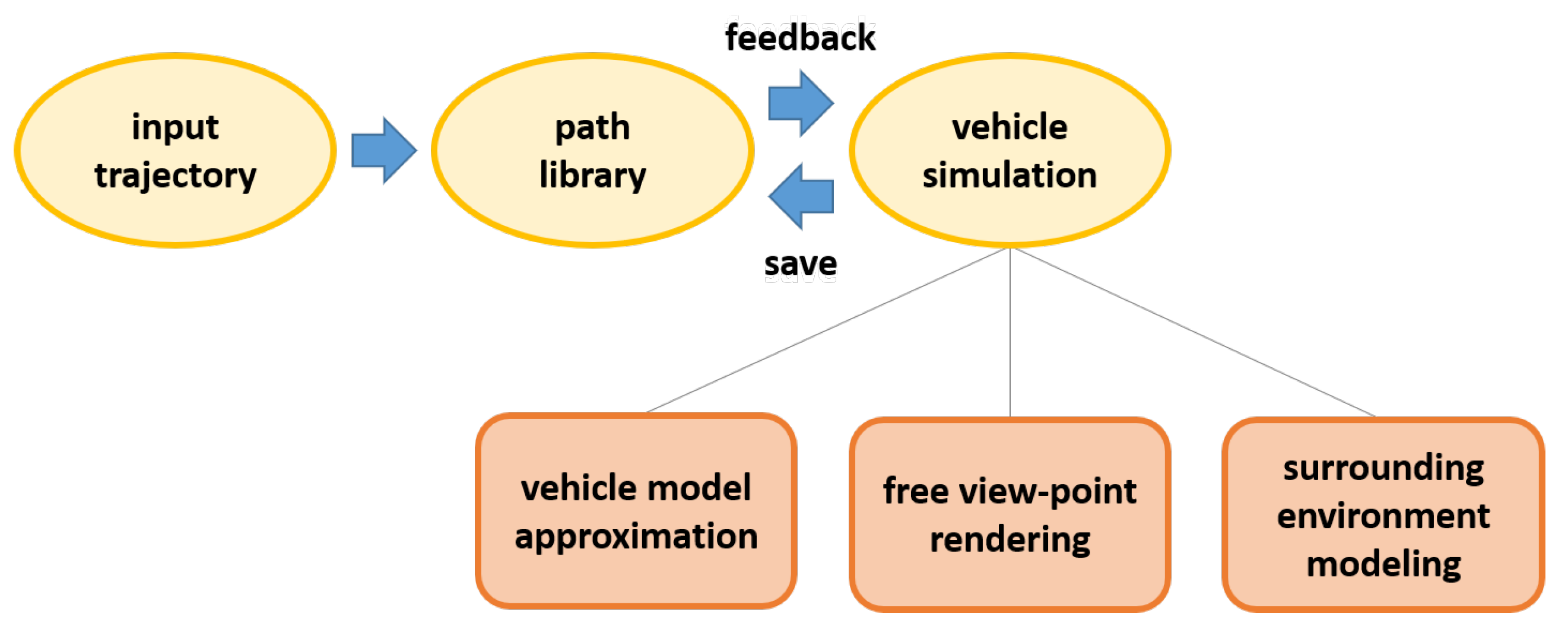
Figure 2 shows the overall process used to simulate our vehicle model on an input trajectory. In the proposed system, a proportional derivative (PD) servo, a popular method in the virtual simulation field, executes the vehicle to run on the trajectory. However, the vehicle often fails to make convincing movements on the trajectory due to physical constraints of the vehicle model. For example, the PD servo-based simulation considers only internal forces such as torque on wheels. If external forces such as gravity and friction are introduced, the simulated vehicle can diverge from the input trajectory. For this, the proposed system splits the input trajectory into several segments and uses a path library to execute the simulation for each segment. This process is iterated until the optimized trajectory is searched or generated for each input segment.

4.1. Vehicle Control

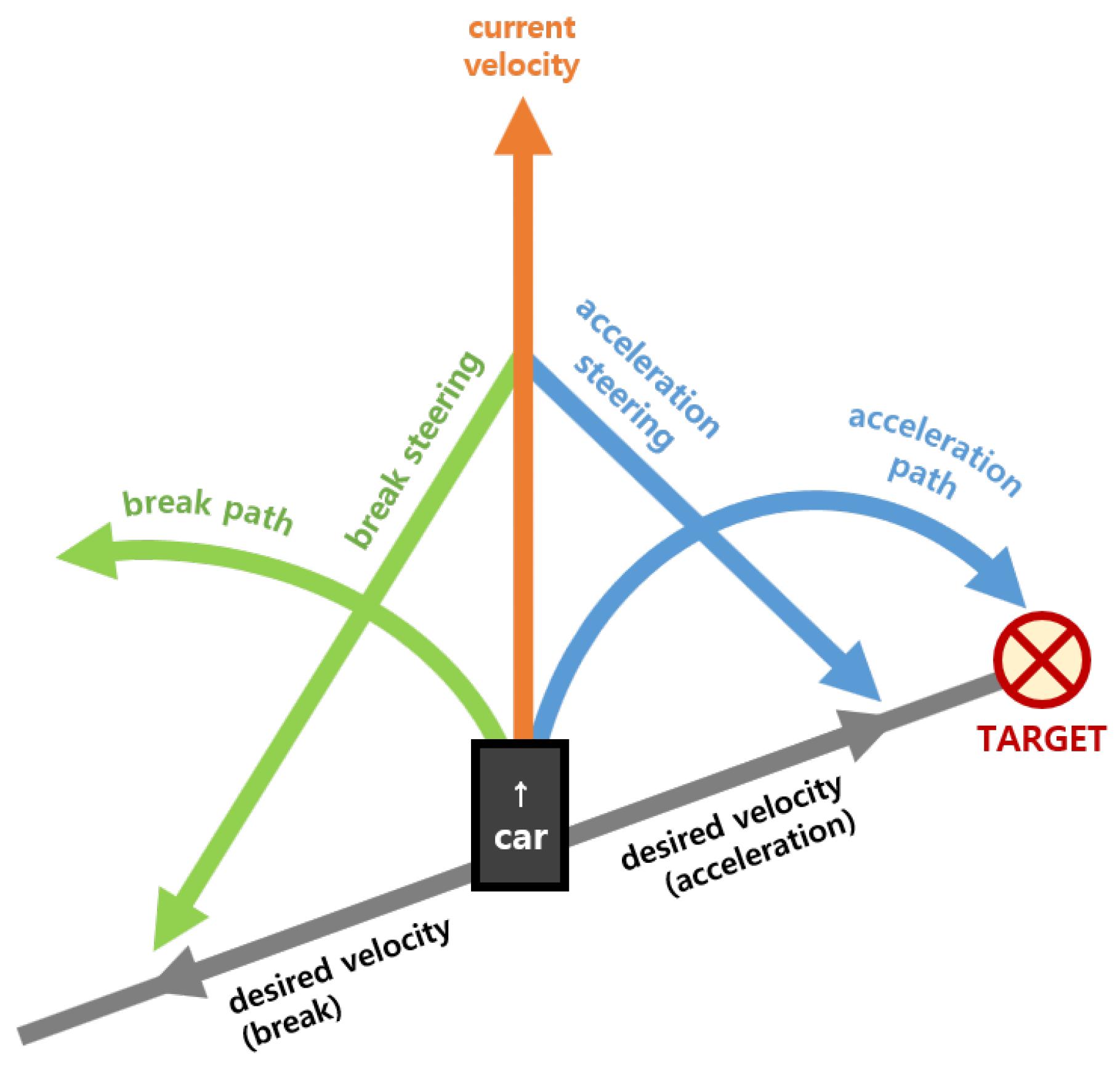
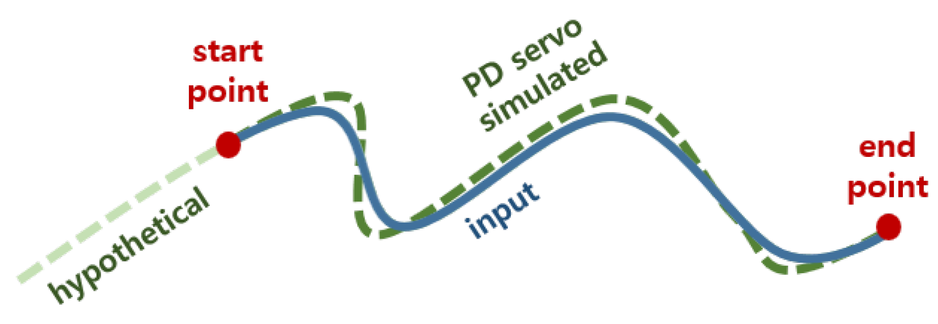
Given an input trajectory, a vehicle runs on a line or a curve with a specified period of time (or frames). For example, given a long trajectory and a fixed time, the vehicle moves with a high velocity while it moves more slowly on a shorter trajectory. In the physics-based simulation system, the PD servo estimates proper torque to steer the vehicle toward the target point. The direction and velocity of the wheels are controlled by forcing the vehicle to follow the input trajectory as closely as possible. Figure 3 shows the directional and velocity changes of the vehicle to steer toward the target point. At every frame, the PD servo acquires the current state of direction and velocity of the vehicle on the trajectory and compares them with future states for the next several frames (i.e., next three frames). At the starting moment, the system assumes that the vehicle requires a certain period to align itself with the input trajectory. For this, a hypothetical trajectory is generated at the starting moment of the simulation and concatenated to the input trajectory, which allows directional change and velocity increase before the vehicle enters the input trajectory with proper direction and velocity. For a smooth transition between those trajectories, the ending point of the hypothetical trajectory becomes the starting point of the input trajectory as shown in Figure 4.
When the vehicle enters the input trajectory, the changes in direction and velocity are estimated from the positional and angular differences of wheels on the trajectory between the current frame, c, and the target frame, t, respectively. For example, if the trajectory from the current position to the target position is close to a straight line, the steering unit controls the direction of wheels to be equal to the direction of a vehicle body. If the trajectory from the current position to the desired position is a curve, the steering unit makes the direction of wheels different from the body direction. The angle difference between wheels and body is estimated by the gradient of the trajectory. The change of velocity is determined by calculating the torque value τ (N·m), as follows:
τ = k ( P t P c ) R w ,
where τ is the rotational torque value required to change from current state to target state, P t is target position of vehicle, P c is current position of vehicle, R w is radius of wheels, and k is a constant gain value of the PD servo. For each frame, the directional and velocity changes are applied to the wheels to maintain the vehicle on the input trajectory. However, frequent changes of torque values for each frame can cause undesired artifacts such as jittering and lagging of vehicle. Moreover, the influence of external forces such as gravity and friction are not considered in Equation (1), which causes directional and positional differences between the simulated and input trajectories. For these reasons, the proposed system splits the input trajectory into several segments and tries to search an optimal trajectory for each segment in an iterative way, as described in the next section.

4.2. Trajectory Optimization

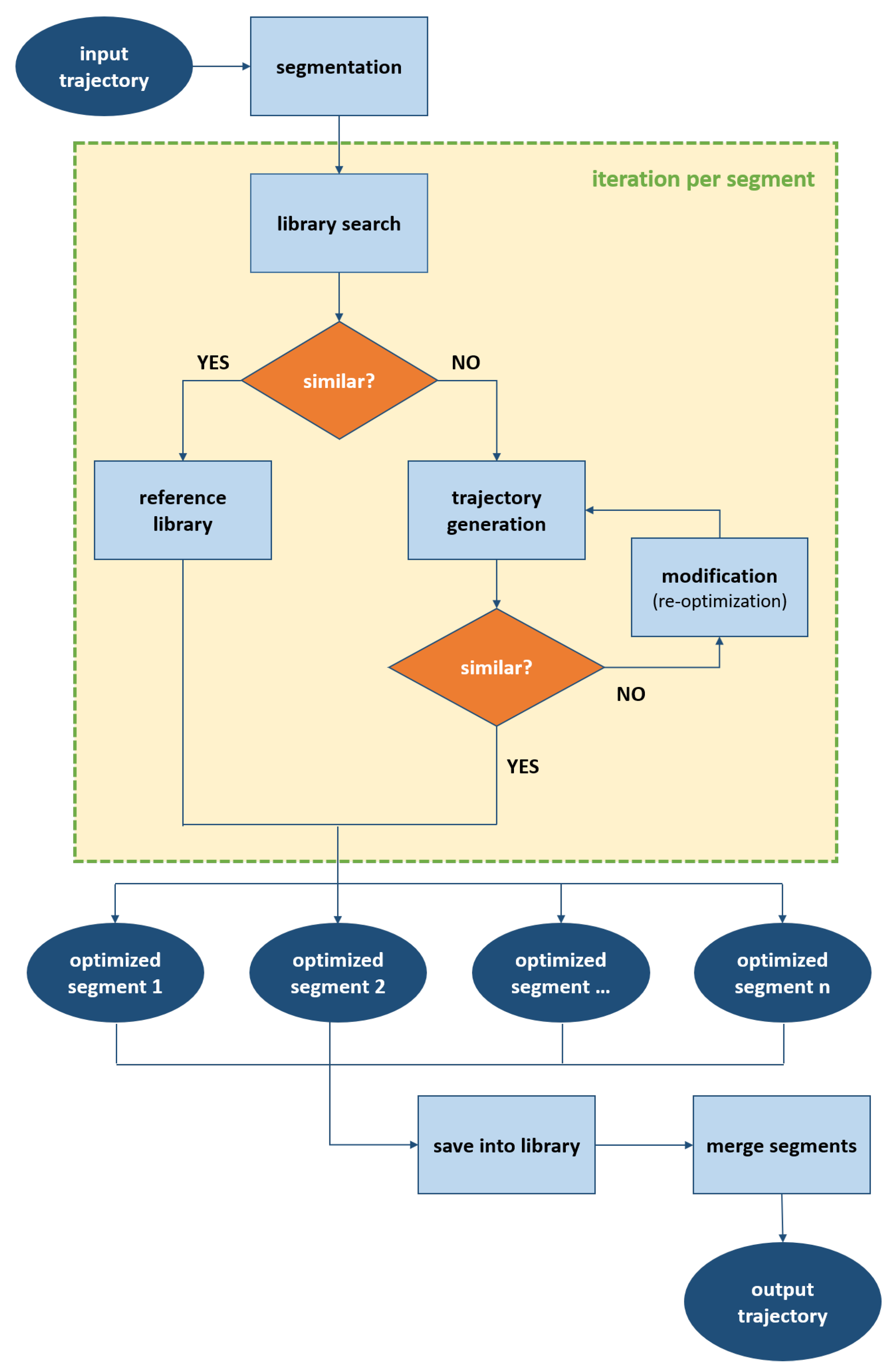
The controls of a real vehicle on a ground path are limited by various physical constraints such as mass, size, wheel motion, etc. For example, the car cannot make sudden turns on sharp curvatures of the input trajectory. In the proposed system, an optimized trajectory that is physically derivable and as similar as possible to the input trajectory is generated via an iterative search method as shown in Figure 5.
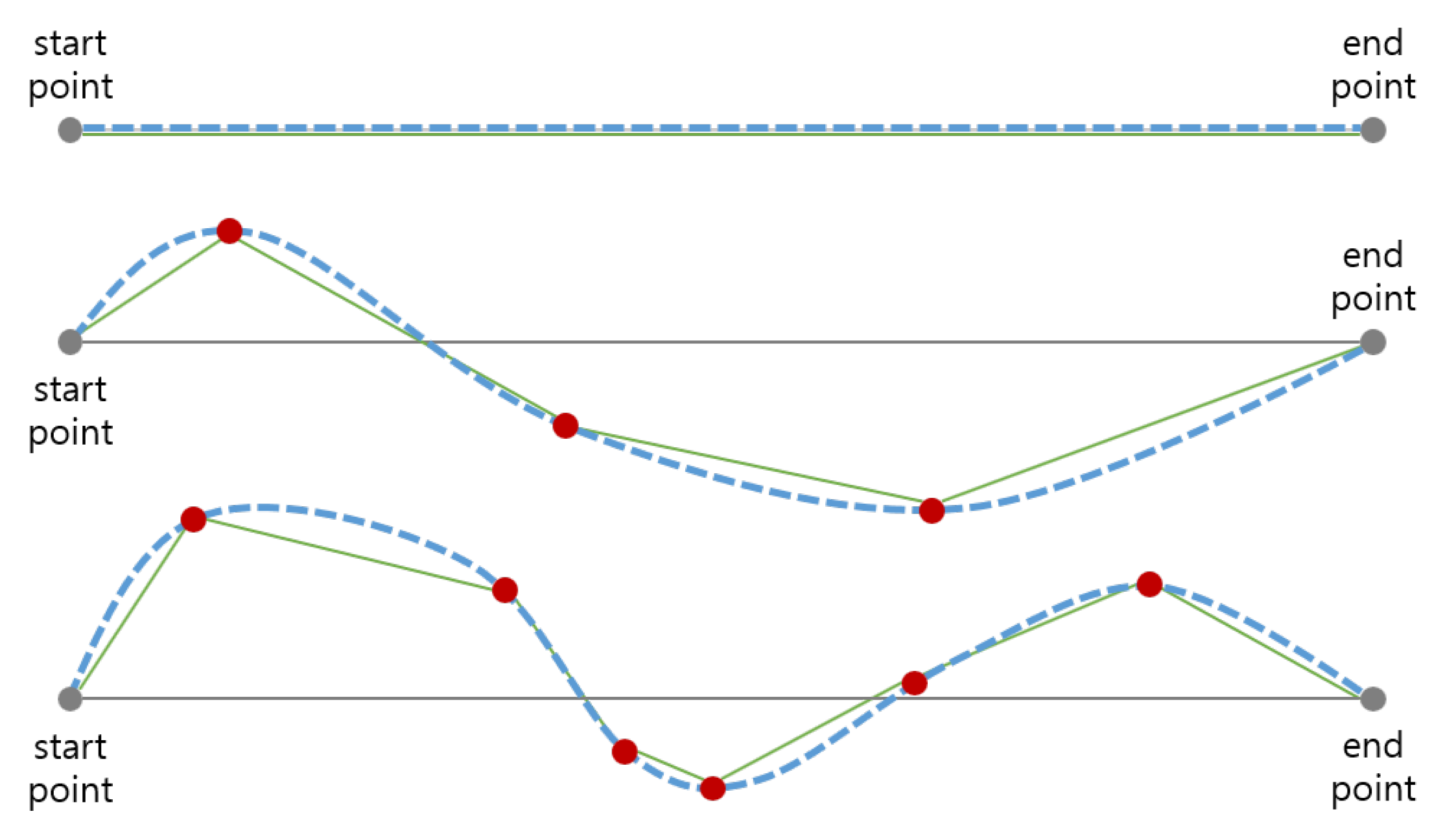
As a preprocessing step, the input trajectory is segmented into several pieces based on the local maximum and minimum points and reflection points. Each of the local maximum and minimum points indicates a moment of gradient switch between positive and negative values, while each of the reflection points indicates a moment of misalignment between the directions of wheels and vehicle body. Figure 6 shows various input trajectories with segmented points. If s i is the ith segment curve on the input trajectory, there is no direction change for wheels on s i , making the simulation process more efficient than one uses the whole trajectory. Given the start and end points of s i , P s , and P e , an initial torque value is estimated from Equation (1) and is averaged by the number of frames between the two points, N τ frames. To reach P e with a proper alignment of wheels, the turning direction, D (m), and its angle, θ D (rad), are estimated as follows:
D = d u p · u × d f w , θ D = c o s 1 ( u · d f w u d f w ) ,
where u = P e P c , and d u p and d f w are the up and forward directions of the vehicle at the current frame, respectively. Here, the vehicle turns right if D > 0 , turns left if D < 0 , and goes straight if D = 0 .
Let s ^ i be a curve simulated by the vehicle based on the direction decided by Equation (2) and the velocity controlled by the PD servo. Due to external forces such as gravity and friction, the end of s ^ i can be different from the end of s i . To minimize this offset, we introduced an optimization process in a multi-stage scheme as shown in Figure 7. This optimization process is implemented by reducing errors in an iterative way until the similarity between two curves is over a user-specified threshold, δ S . The details of the optimization scheme will be described in the next paragraph. For the next segment, s i + 1 , the end conditions (i.e., the vehicle direction and velocity) of s i should be close enough to the start conditions of s i + 1 ; otherwise, the vehicle cannot make a smooth transition between two segments. Another similarity threshold value, δ T , is set such that s ^ i is regenerated by the simulation process if δ T is not satisfied. In our experiments, both δ S and δ T are set at 0.9 for convincing simulation results; however, they can be adjusted based on user preferences.
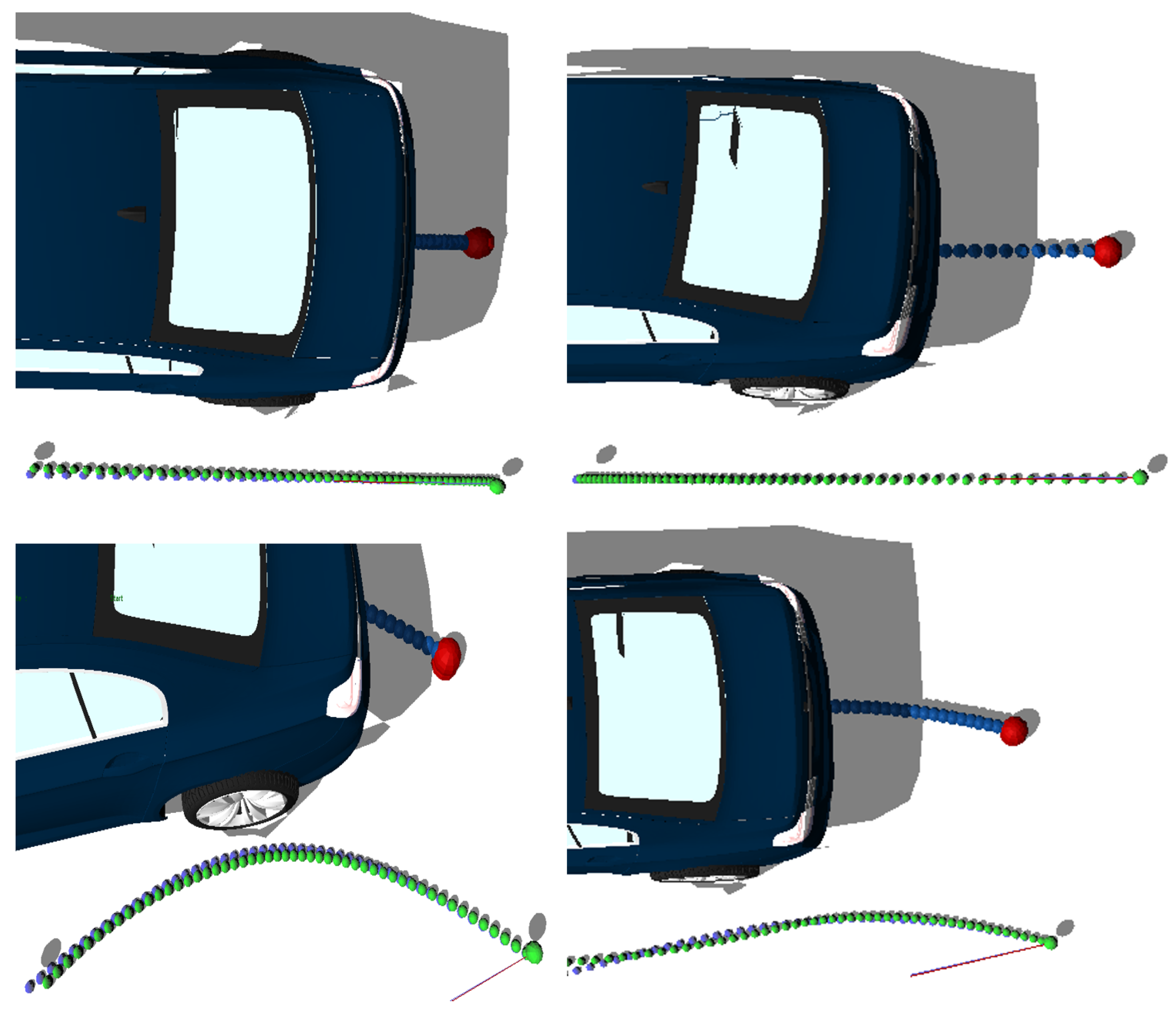
Given multiple trajectory segments, the vehicle direction and velocity at the end point of the current segment become the starting point of the next segment. To simulate a vehicle following the input trajectory as closely as possible, the difference between the direction and velocity at the end point of each segment should be minimized between s i and s i ^ . When there is a large difference between these values, our approach restarts the simulation at the previous end point until the difference is within the threshold value. Motivated by the work of Kwon and Hodgins [27], our approach adopts a multi-stage optimization scheme that looks up previous segments when a current segment is optimized, as shown in Figure 8. In the first stage, the hypothetical trajectory (in Section 4.1) is first looked up for the optimization.

4.3. Trajectory Search

As s ^ i is generated for s i , it can be time-consuming to estimate s ^ i when there are many segments on the input trajectory. Archiving s ^ i into a path library, the proposed system can accelerate the simulation process by searching s ^ j on the next input segment, where j [ 1 , , N L ] and N L is a size of the library. As shown in Figure 5, the proposed system compares the start states of the vehicle between s ^ j and s i as follows:
m i n ( v ^ j , v i ) m a x ( v ^ j , v i ) δ L 1 , m i n ( L ^ j , L i ) m a x ( L ^ j , L i ) δ L 2 , m i n ( θ ^ j , θ i ) m a x ( θ ^ j , θ i ) δ L 3 ,
where v ^ j and v i are the velocity of the vehicle at P s of s ^ j and s i , respectively. Similarly, L ^ j and L i are the length and θ ^ j and θ i are the curve slope with respect to the tangent to P s of s ^ j and s i , respectively. Here, δ L 1 , 2 , 3 are user-specified thresholds that are set to 0.9 in our simulation. At P e of the segments, if P e is a reflection point, the direction of the wheels is checked against the vehicle body. If there are multiple candidates produced by Equation (3), the proposed system iterates the search process at P N P / k , where N P is the total number of simulated positions on s i and k [ 2 , 3 , 4 , , N P ] . It is noteworthy that the library is initially empty in the first simulation; however, it grows larger in a short period as the simulation reiterates various input segments. Figure 9 shows a comparison of the input and simulated segment curves that are searched from the library.

4.4. Contact with Ground Surface

The proposed system keeps the wheels in contact with the road surface by satisfying the collision restraints of the LCP solver [28]. For example, the value of the contact force should change within the friction cone, the value of the relative velocity of the contact point should change within the velocity cone, and the velocity is zero if the contact force is zero. However, if a wheel rotates at high speed, the fixed contact point at the current frame can be located below the ground level in the next frame during a single simulation step (i.e., 1 3000 s). This results in undesirable artifacts such as wheel slide and penetration when a general physics engine is used. We overcome this problem by setting the constraints in the LCP with the contact point at the next time step as follows:
p ˙ = p + ( v t ) ,
where p ( R 3 ) is the deepest penetrating point, v is the linear velocity of the wheel’s center of mass (COM), t is the time step of the simulation, and p ˙ ( R 3 ) is the contact point after time t.

5. Vehicle Deformation

To keep vehicle running on the ground all the time, the proposed system keeps detecting a static collision between wheels and ground plane without penetration. For computational efficiency, a simple square box that covers the vehicle body is used for any detection from outside. Using this collision detector, the vehicle body starts to deform if any object goes into the box or stops deforming if a part of the body goes out of the box.
In the event of a vehicle crash, the box collision detector calculates the direction and magnitude of collision impulse for each frame. Based on the impulse force, the key body parts such as front bumper and wheels translate their positions and change their shapes to represent the surface deformation. For smooth deformation, the linear blend skinning (LBS) is a method that transforms vertices inside a single mesh by a blend of multiple transforms. It is widely used due to its simple implementation and fast performance. Given a mesh model, it decides the vertex position according to the final transformation matrix, which is the result of multiplication of all required transformation matrices (scaling, translating, rotating), as follows:
p ¯ i = j = 1 N B w i j T j p i ,
where p i ( R 3 ) is the vertex position of the ith mesh in resting pose, p ¯ i ( R 3 ) is the vertex position after deformation, N B is the number of bones, T j is a 4 × 4 matrix that defines a global transformation of the jth bone from its rest pose, and w i j is a scalar weight at the ith vertex associated with the jth bone. As the LBS method does not consider each property of the required transformations, it causes the candy wrapper problem which produces an visual artifact such as an intermittent twisting surface.
To deform the surface of the vehicle model, the proposed system adopts the dual quaternion skinning (DQS) method, which is a skinning algorithm based on a linear combination of dual quaternions [29]. In this method, DQS decides the vertex position with dual quaternion values which are used for interpolation instead of T j in Equation (5). Each quaternion includes rotational and translational transformations as follows:
q ˙ = i = 1 N B w i q ˙ i | i = 1 N B w i q ˙ i | ,
where q ˙ i ( S 3 ) is the bone’s dual quaternions (transformations) weighted by w i . It is notable that Equation (6) estimates the two transformations separately and does not have any scaling factor, providing a faster computation without the candy wrapper artifact.
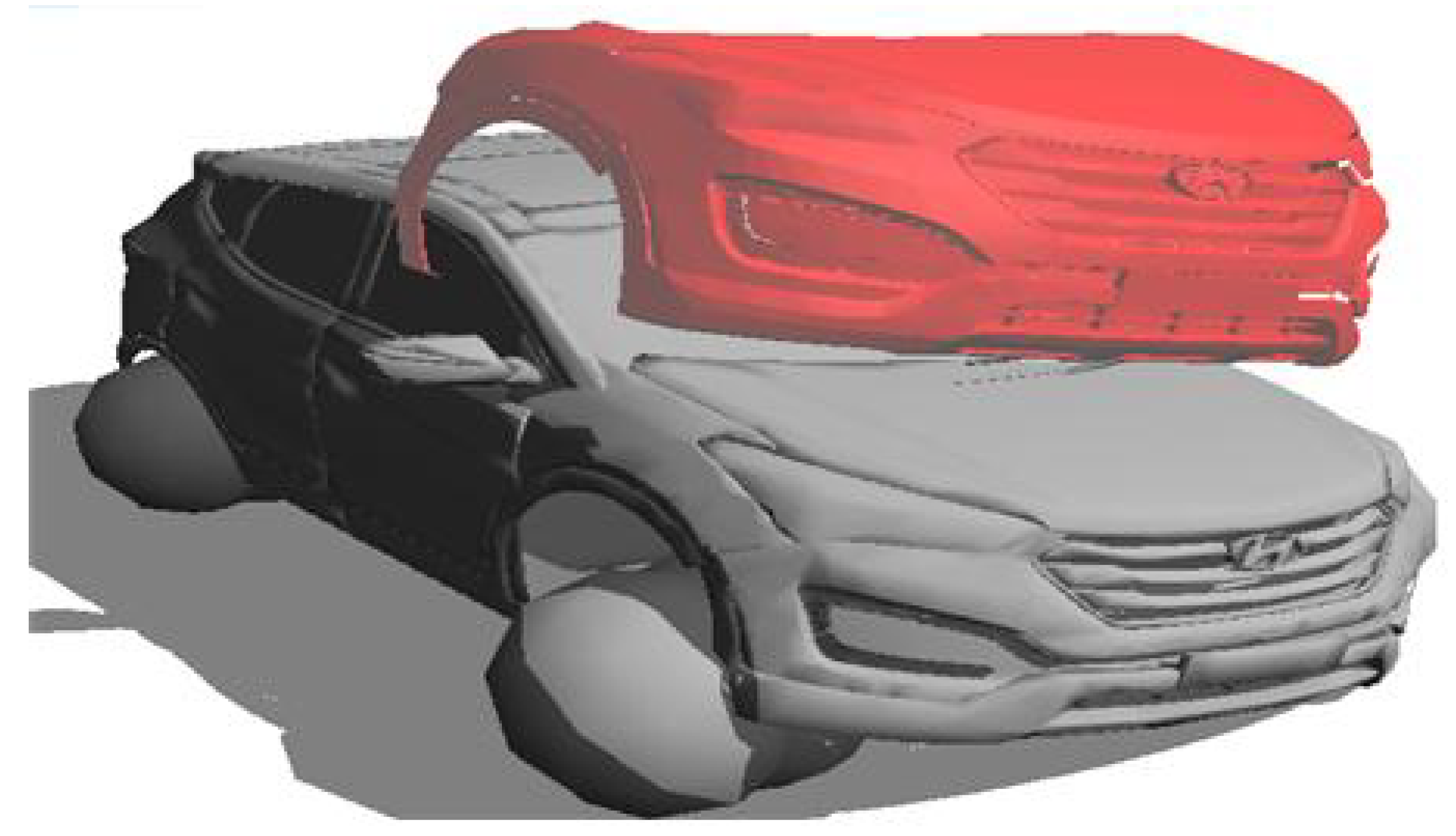
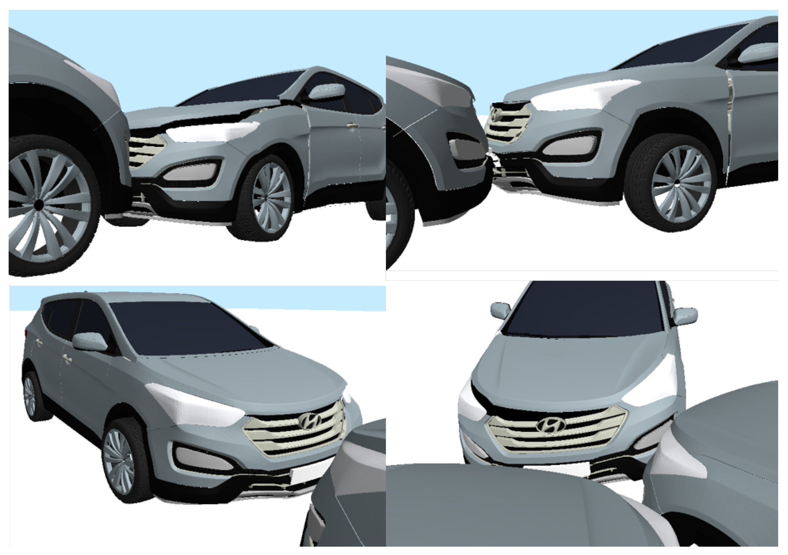
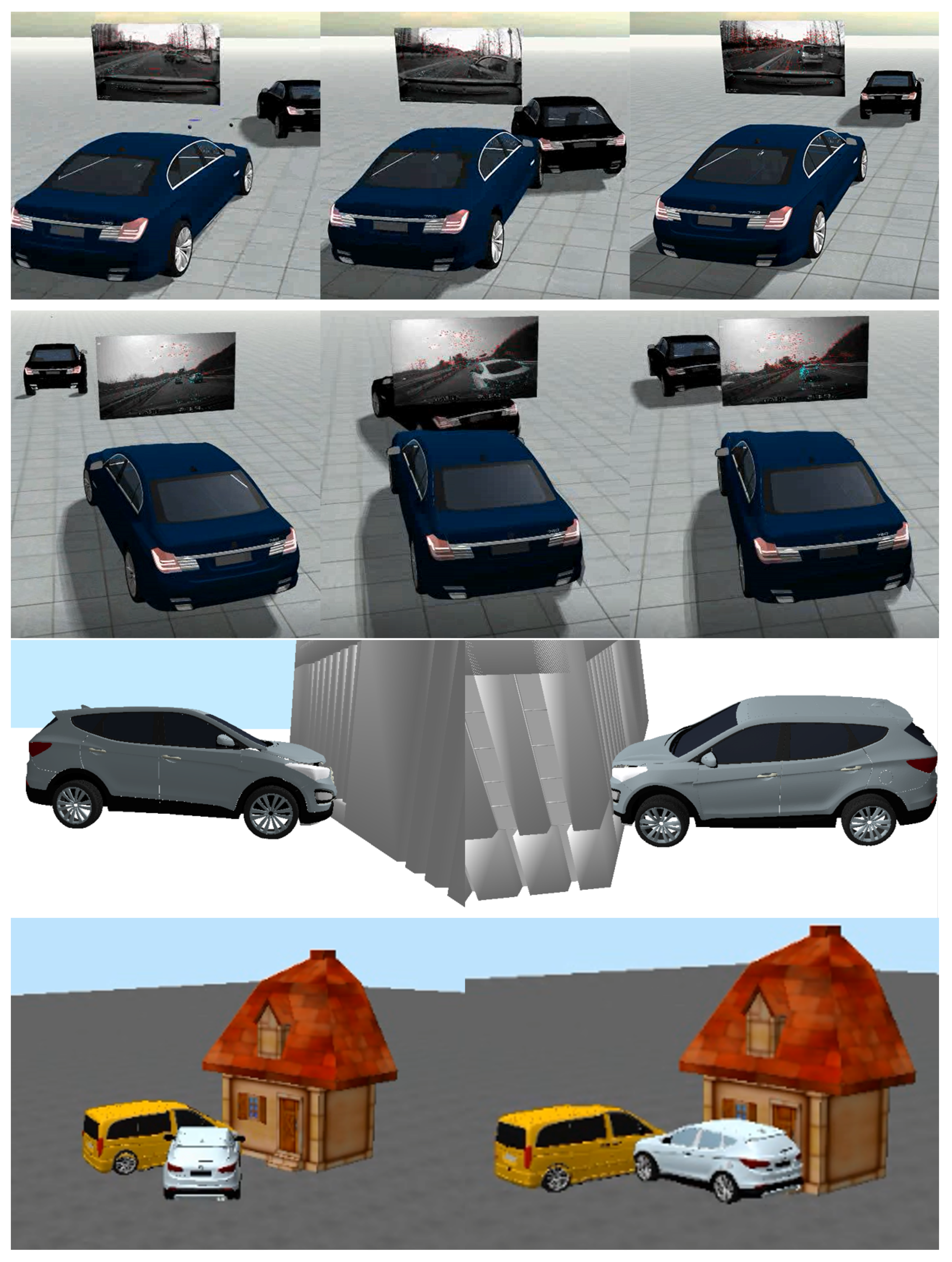
Figure 10 shows the part of the vehicle body deformed by the impulse force. In the figure, the left body part, which is described in Section 3, is lifted and dented based on the empirical values. During bumper deformation, the translational axis of the wheels is moved together with the bumper to prevent any self-penetration, as shown in Figure 11. Figure 12 shows an example of a crash scene between two vehicles in which the bumper is moved backward and bent.

6. Experimental Results

Experiments were performed on an AMD FX-8120 3.1 GHz PC with 24 GB DDR4 memory and AMD Cedar graphics under the Ubuntu operation system (a version of 16.04.6 LTS 64-bit). The proposed system uses OpenHRP [30] and Bullet [31] which provide various software components and calculation libraries for dynamic simulation and collision detection, respectively. The proposed system is best understood through examples of its uses, as described in the subsequent sections. The accompanying video is located at [32].

6.1. Simulation Tool

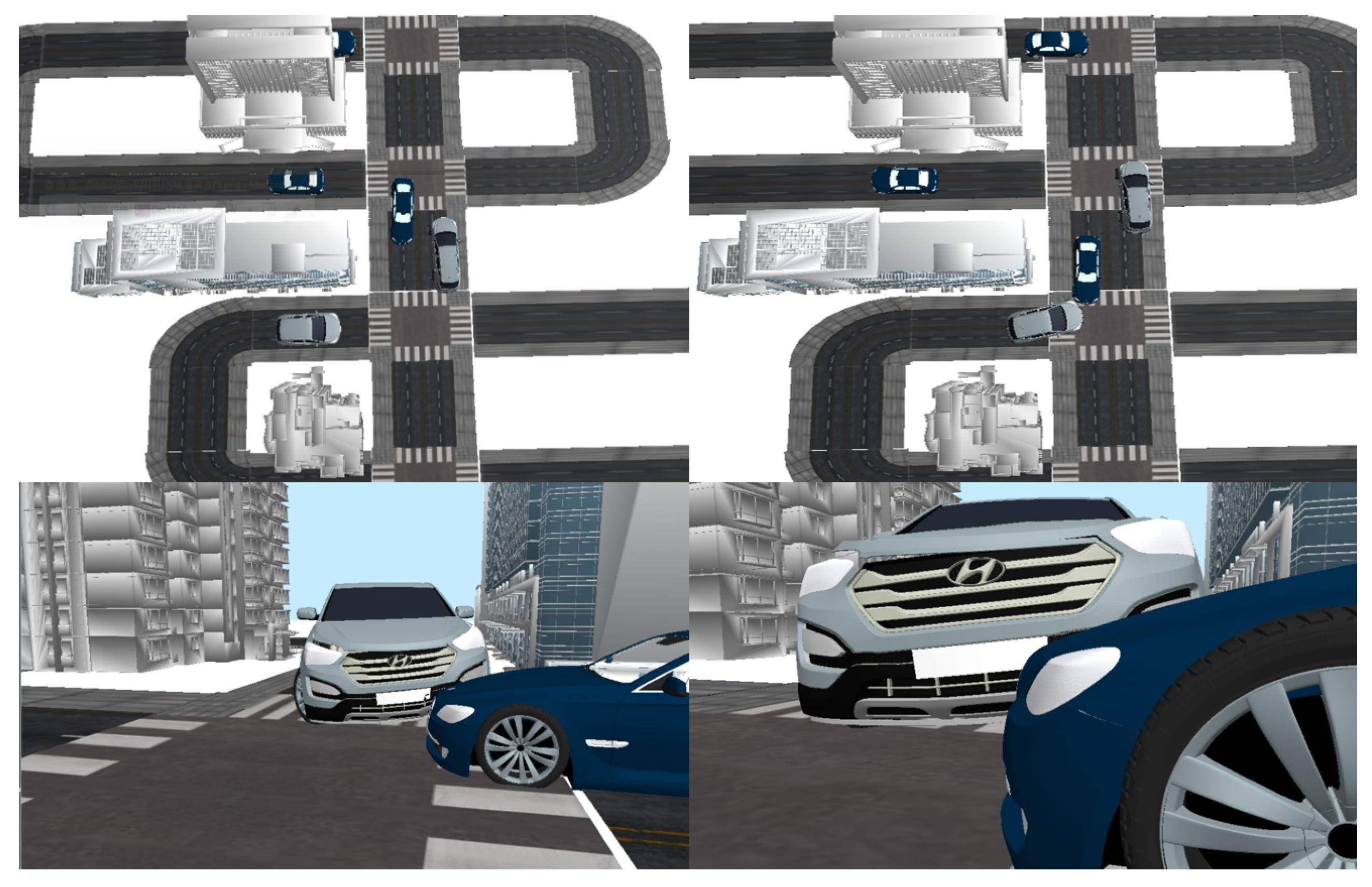
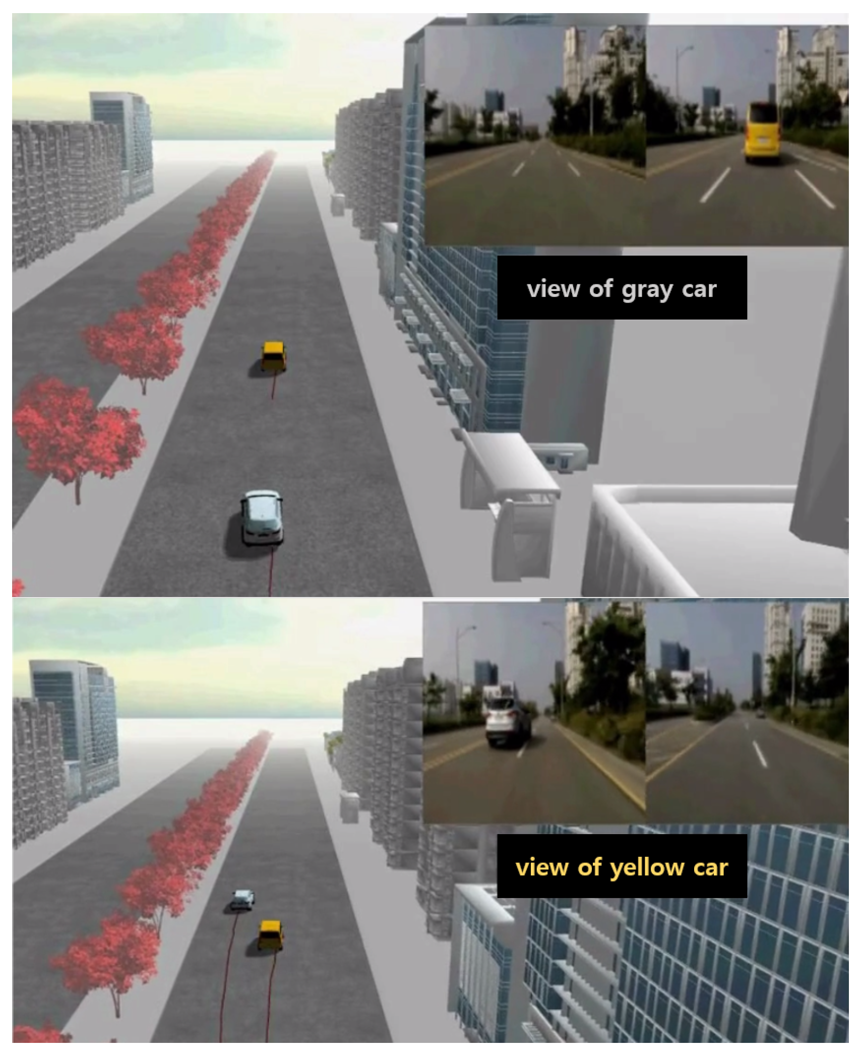
The proposed system provides an interactive tool for physics-based vehicle simulation and creates various traffic scenes. Using this tool, a user can create a background scene with multiple vehicles and specify an individual trajectory for each vehicle. In the simulation, the vehicles keep running along the specified trajectories, passing each other, changing lanes, and crashing into each other depending on the trajectory conditions as shown in Figure 13 and Figure 14.
It is noteworthy that the vehicle can hit not only other vehicles, but also surrounding objects such that the user can create a multiple pile-up scene. In addition, a specific scene frame can be viewed from any viewpoint via the provided interface. This is useful to observe special events such as vehicle crash scenes, as shown in Figure 15.

6.2. Simulation Using GPS Data

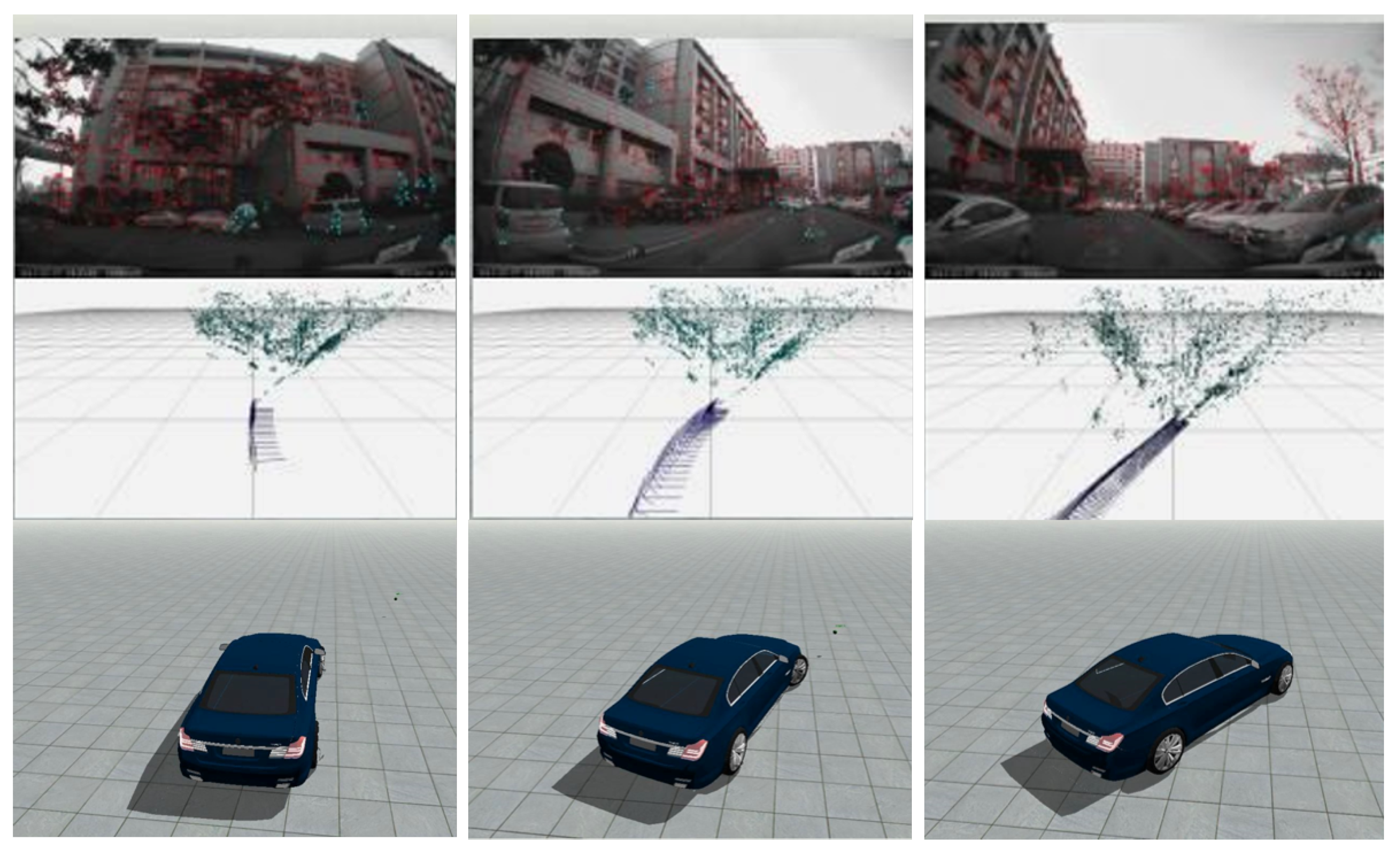
Using global position system (GPS) data captured from a surveillance camera (a.k.a. dashboard camera), a traffic scene similar to a real situation can be generated without an input trajectory specified by user. Using the Kanade–Lucas–Tomasi (KLT) feature tracker, which is a local search using gradients weighted by an approximation to the second derivative of the image, a set of feature points is detected and tracked from a sequence of camera images [33]. For each frame, the 3D positions of the scene camera are estimated using the structure from motion (SFM) method that estimates 3D structure from the 2D image sequences by tracking feature points [34]. Using a least-squares fitting method, an input trajectory can be estimated from the GPS data extracted from dashboard camera and used to generate traffic scene, as shown in Figure 16. Compared to the real scene captured from the camera, the simulated scene shows convincing movements of vehicles in terms of physical properties such as velocity and direction.

7. Conclusions

In this paper, we introduced a novel system for physics-based vehicle simulation from input trajectory. While previous approaches focus on representing large-scale traffic flow, the proposed system approximates the physical movements of a real vehicle using a PD servo and deforms its shape to generate convincing interaction with other objects. Using the path library, the system avoids expensive simulation calculation and creates responsive vehicle scenes where multiple vehicles run on the specified paths, change lanes, pass each others, and collide with other objects. Utilizing camera data for an input trajectory, such a responsive simulation is useful for reproducing real traffic scenes such as reenacting a car accident for review. In the proposed system, the overall simulation process is fully automated and designed for a general user who is not familiar with the dynamic properties of moving vehicles.
The current system archives the simulated results into a library to reduce the optimized trajectory search time. As the size of the library grows larger, there can be many similar trajectories stored in it, which can reduce the search time. By comparing the shape similarity between the trajectories, we plan to remove any redundant trajectories and maintain the optimal size of the library. In addition, the weight skinning method used for the deformation only approximates the mesh surface shape. For better visual quality, a more sophisticated method can be applied for the deformation process. Finally, the proposed system mainly attempts to generate traffic scenes with several vehicles. Its performance can degrade for large traffic scenes with tens or hundreds of vehicles. For such large-scaled simulation, vehicles on input trajectories can be parallelized to expedite the optimization process. Handling a dynamic trajectory to generate extreme scenes like car acrobatics is also an ongoing work.

Author Contributions

Conceptualization, D.K. and J.J.; Data curation, D.K. and J.J.; Formal analysis, D.K., J.J., S.-w.K., T.K., and Y.K.; Funding acquisition, T.K.; Investigation, J.J. and Y.K.; Methodology, D.K., J.J., and Y.K.; Project administration, T.K.; Software, J.J. and S.-w.K.; Supervision, T.K. and Y.K.; Validation, S.-w.K.; Visualization, D.K.; Writing—original draft, D.K. and Y.K.; Writing—review and editing, Y.K.

Funding

This research was supported by the Basic Science Research Program through the National Research Foundation of Korea (NRF) funded by the Ministry of Education(NRF-2017R1D1A1B03034889) and by Institute for Information & communications Technology Promotion (IITP) grant funded by Korea government (MSIT) (No. 2019-0-01849, Development of Core Technology for Real-Time Image Composition in Unstructured In Outdoor Environment).

Conflicts of Interest

The authors declare no conflict of interest.

Abbreviations

The following abbreviations are used in this manuscript:
PDProportional derivative
LCPLinear complementarity problem
LBSLinear blend skinning
DQSDual quaternion skinning
GPSGlobal position system
KLTKanade–Lucas–Tomasi
SFMStructure from motion

References

  1. Schaal, S.; Kotosaka, S.; Sternad, D. Nonlinear dynamical systems as movement primitives. In Proceedings of the IEEE International Conference on Humanoid Robotics, MIT, Cambridge, MA, USA, 7–8 September 2000; pp. 1–11. [Google Scholar]
  2. Schaal, S.; Peters, J.; Nakanishi, J.; Ijspeert, A. Learning movement primitives. In Robotics Research the Eleventh International Symposium; Springer: Berlin/Heidelberg, Germany, 2005; pp. 561–572. [Google Scholar]
  3. Kobilarov, M.; Crane, K.; Desbrun, M. Lie group integrators for animation and control of vehicles. ACM Trans. Graph. 2009, 28, 16. [Google Scholar] [CrossRef]
  4. Sewall, J.; Wilkie, D.; Merrell, P.; Lin, M.C. Continuum Traffic Simulation. Comput. Graph. Forum 2010, 29, 439–448. [Google Scholar] [CrossRef]
  5. Sewall, J.; Wilkie, D.; Lin, M.C. Interactive hybrid simulation of large-scale traffic. Acm Trans. Graph. 2011, 30, 135. [Google Scholar] [CrossRef]
  6. Garcia-Dorado, I.; G Aliaga, D.; V Ukkusuri, S. Designing Large-Scale Interactive Traffic Animations for Urban Modeling. Comput. Graph. Forum 2014, 33, 411–420. [Google Scholar] [CrossRef]
  7. Kallmann, M.; Lemoine, P.; Thalmann, D.; Cordier, F.; Magnenat-Thalmann, N.; Ruspa, C.; Quattrocolo, S. Immersive vehicle simulators for prototyping, training and ergonomics. In Proceedings of the IEEE Computer Graphics International, Tokyo, Japan, 9–11 July 2003; pp. 90–95. [Google Scholar]
  8. Tan, J.; Gu, Y.; Liu, C.K.; Turk, G. Learning bicycle stunts. ACM Trans. Graph. 2014, 33, 50. [Google Scholar] [CrossRef]
  9. Galin, E.; Peytavie, A.; Maréchal, N.; Guérin, E. Procedural Generation of Roads. Comput. Graph. Forum 2010, 29, 429–438. [Google Scholar] [CrossRef]
  10. Stewart, D.; Trinkle, J.C. An implicit time-stepping scheme for rigid body dynamics with coulomb friction. In Proceedings of the IEEE International Conference on Robotics and Automation (ICRA’00), San Francisco, CA, USA, 24–28 April 2000; Volume 1, pp. 162–169. [Google Scholar]
  11. Lötstedt, P. Numerical simulation of time-dependent contact and friction problems in rigid body mechanics. SIAM J. Sci. Stat. Comput. 1984, 5, 370–393. [Google Scholar] [CrossRef]
  12. Baraff, D. Coping with friction for non-penetrating rigid body simulation. ACM Siggraph Comput. Graph. 1991, 25, 31–41. [Google Scholar] [CrossRef]
  13. Baraff, D. Fast contact force computation for nonpenetrating rigid bodies. In Proceedings of the 21st Annual Conference on Computer Graphics and Interactive Techniques, Orlando, FL, USA, 24–29 July 1994; pp. 23–34. [Google Scholar]
  14. Trinkle, J.C.; Pang, J.S.; Sudarsky, S.; Lo, G. On Dynamic Multi-Rigid-Body Contact Problems with Coulomb Friction. ZAMM-J. Appl. Math. Mech. FÜR Angew. Math. Und Mech. 1997, 77, 267–279. [Google Scholar] [CrossRef]
  15. Erleben, K. Velocity-based shock propagation for multibody dynamics animation. ACM Trans. Graph. 2007, 26, 12. [Google Scholar] [CrossRef]
  16. Kaufman, D.M.; Sueda, S.; James, D.L.; Pai, D.K. Staggered projections for frictional contact in multibody systems. ACM Trans. Graph. 2008, 27, 164. [Google Scholar] [CrossRef]
  17. Otaduy, M.A.; Tamstorf, R.; Steinemann, D.; Gross, M. Implicit Contact Handling for Deformable Objects. Comput. Graph. Forum 2009, 28, 559–568. [Google Scholar] [CrossRef]
  18. Coros, S.; Martin, S.; Thomaszewski, B.; Schumacher, C.; Sumner, R.; Gross, M. Deformable objects alive! ACM Trans. Graph. 2012, 31, 69. [Google Scholar] [CrossRef]
  19. Barbič, J.; Popović, J. Real-time control of physically based simulations using gentle forces. ACM Trans. Graph. 2008, 27, 163. [Google Scholar] [CrossRef]
  20. Skouras, M.; Thomaszewski, B.; Coros, S.; Bickel, B.; Gross, M. Computational design of actuated deformable characters. ACM Trans. Graph. 2013, 32, 82. [Google Scholar] [CrossRef]
  21. Liu, L.; Yin, K.; Wang, B.; Guo, B. Simulation and control of skeleton-driven soft body characters. ACM Trans. Graph. 2013, 32, 215. [Google Scholar] [CrossRef]
  22. Tan, J.; Gu, Y.; Turk, G.; Liu, C.K. Articulated swimming creatures. ACM Trans. Graph. 2011, 30, 58. [Google Scholar] [CrossRef]
  23. Wang, Y.; Jacobson, A.; Barbič, J.; Kavan, L. Linear subspace design for real-time shape deformation. ACM Trans. Graph. 2015, 34, 57. [Google Scholar] [CrossRef]
  24. Larsson, T.; Akenine-Möller, T. Efficient collision detection for models deformed by morphing. Vis. Comput. 2003, 19, 164–174. [Google Scholar]
  25. Teschner, M.; Kimmerle, S.; Heidelberger, B.; Zachmann, G.; Raghupathi, L.; Fuhrmann, A.; Cani, M.P.; Faure, F.; Magnenat-Thalmann, N.; Strasser, W.; et al. Collision Detection for Deformable Objects. Comput. Graph. Forum 2005, 24, 61–81. [Google Scholar] [CrossRef]
  26. Kavan, L.; Žára, J. Fast Collision Detection for Skeletally Deformable Models. Comput. Graph. Forum 2005, 24, 363–372. [Google Scholar] [CrossRef]
  27. Kwon, T.; Hodgins, J.K. Momentum-mapped inverted pendulum models for controlling dynamic human motions. ACM Trans. Graph. 2017, 36, 10. [Google Scholar] [CrossRef]
  28. Yamane, K.; Nakamura, Y. A numerically robust LCP solver for simulating articulated rigid bodies in contact. In Proceedings of the Robotics: Science and Systems IV, Zurich, Switzerland, 25–28 June 2008; Volume 19, p. 20. [Google Scholar]
  29. Kavan, L.; Collins, S.; Žára, J.; O’Sullivan, C. Skinning with dual quaternions. In Proceedings of the 2007 Symposium on Interactive 3D Graphics and Games, Seattle, WA, USA, 30 April–2 May 2007; pp. 39–46. [Google Scholar]
  30. OpenHRP3. Available online: http://fkanehiro.github.io/openhrp3-doc/en/index.html (accessed on 10 June 2019).
  31. Bullet Collision Detection & Physics Library. Available online: https://pybullet.org/Bullet/BulletFull/index.html (accessed on 20 March 2019).
  32. Video for Experimental Results. Available online: https://drive.google.com/open?id=1VEkKGmnfz0a2ESw3gJinKaqwPej9QNoD (accessed on 28 October 2019).
  33. Tomasi, C.; Kanade, T. Detection and Tracking of Point Features; Technical Report CMU-CS-91-132; Carnegie Mellon University: Pittsburgh, PA, USA, 1991. [Google Scholar]
  34. Häming, K.; Peters, G. The structure-from-motion reconstruction pipeline–a survey with focus on short image sequences. Kybernetika 2010, 46, 926–937. [Google Scholar]
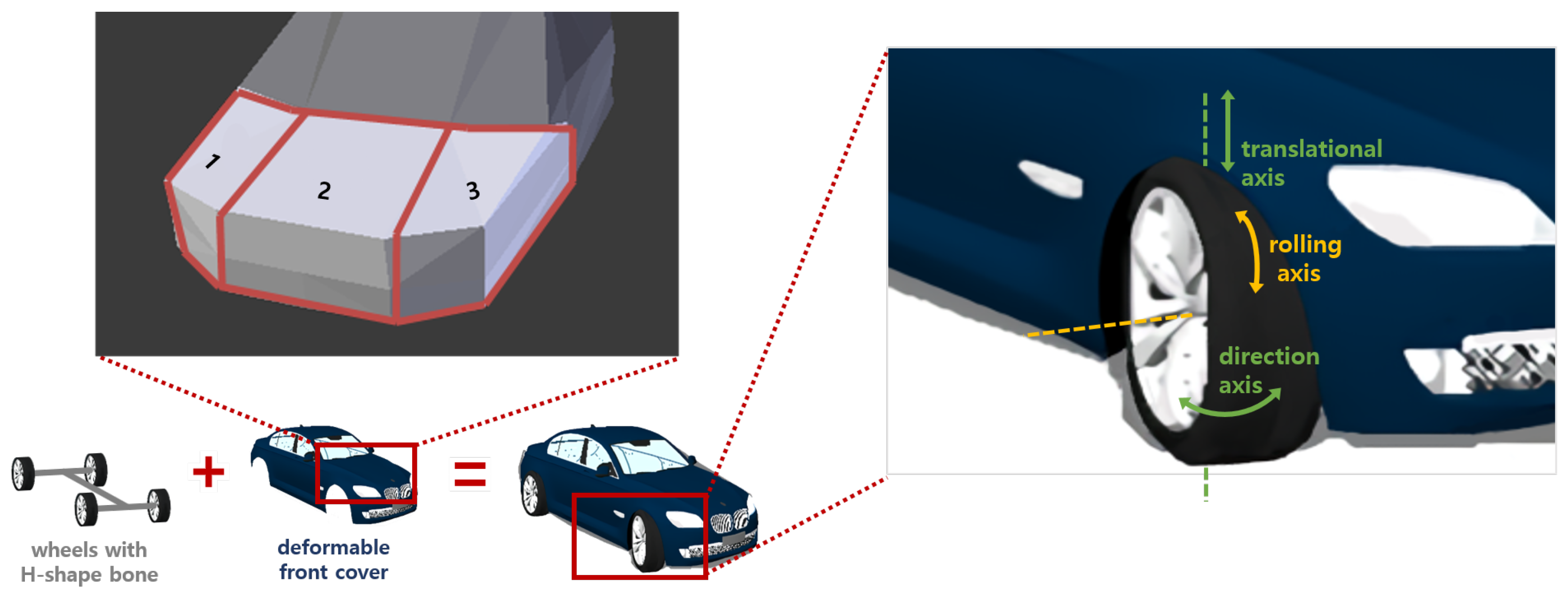
Figure 1. Vehicle model: deformable front cover with rotational and translational axes used for wheel movements.
Applsci 09 04949 g001
Figure 2. Overview of vehicle simulation on input trajectory.
Applsci 09 04949 g002
Figure 3. Steering vehicle toward target point.
Applsci 09 04949 g003
Figure 4. Path simulated by a proportional derivative (PD) servo on hypothetical and input trajectories.
Applsci 09 04949 g004
Figure 5. Overview of generation of optimized trajectory using an iterative search method.
Applsci 09 04949 g005
Figure 6. Segmentation of input trajectories (blue) with local extremes and inflection points (red).
Applsci 09 04949 g006
Figure 7. Trajectory optimization process based on similarity of curve shapes between input and simulated segments.
Applsci 09 04949 g007
Figure 8. Trajectory optimization with multi-stages: At each iteration, current segments (green) are newly optimized based on previously optimized segments (yellow), where their shape can be modified depending on difference of vehicle conditions (direction and velocity) at the end points between the input and simulated trajectories.
Applsci 09 04949 g008
Figure 9. Comparison between input (blue) and simulated segments (green) searched in a path library.
Applsci 09 04949 g009
Figure 10. Comparison between translated (gray) and deformed bumper (red).
Applsci 09 04949 g010
Figure 11. Comparison between deformed bumper without translated wheels (left) and with translated wheels (right).
Applsci 09 04949 g011
Figure 12. Vehicle crash scene using a weighted skinning method.
Applsci 09 04949 g012
Figure 13. Traffic scene created with background and multiple vehicle models.
Applsci 09 04949 g013
Figure 14. Traffic scene with two vehicles passing each other.
Applsci 09 04949 g014
Figure 15. Various crash scenes.
Applsci 09 04949 g015
Figure 16. Input trajectory estimated from GPS data extracted from dashboard camera.
Applsci 09 04949 g016