Abstract
This paper focuses on field measurements and analyses of train-generated wind loads on wind barriers (3.0 m height and porosity 0%) with respect to different running speeds of the CRH380A EMU vehicle. Multi-resolution analysis was conducted to identify the pressure distribution in different frequency bands. Results showed that the wind pressure on the wind barrier caused by train-induced wind had two significant impacts with opposite directions, which were the “head wave” and “tail wave”. The peak wind pressure on the wind barrier was approximately proportional to the square of the speed of the train, and the peak wind pressure decreased rapidly along the wind barrier height from the bottom of the wind barrier. The maximum wind pressure occurred at the rail surface height. Furthermore, results of the multi-resolution analysis illustrated that the energy of the frequency band from 0 to 2.44 Hz accounted for 94% of the total energy. This indicated that the low-frequency range component of the wind pressure dominated the design of the wind barrier. The frequency of pulse excitation of train-induced wind loads may overlap with the natural frequency of barriers, and may lead to fatigue failure due to cyclic loads generated by the repeated passage of high-speed trains. In addition, the speed of the train had a negligible effect on the energy distribution of the wind pressure in the frequency domain, while the extreme pressure increased slightly with the increase of the speed of the train.
1. Introduction
With the rapid development of the high-speed railways, the safety and comfort of high-speed trains under strong winds has drawn extensive attention worldwide [1,2,3,4,5]. Matschke et al. [6] proposed three strategies to improve the running safety of a train under strong winds; namely, optimization of the aerodynamic shape, operation management, and installation of wind barriers. However, optimization of the aerodynamic shape is impractical for existing trains. Operation management will bring about, for instance, speed limitations and temporary out of service times, which will lead to train delays and inefficiency in transportation. Moreover, this goes against the superiority of high-speed trains, which promote all-weather, fast, and on-time operations. In light of this, wind barriers can create a relatively low-wind environment for high-speed trains. The wind barrier is, therefore, an effective measure to improve the safety of high-speed trains in existing railway lines. In recent years, significant achievements on wind barriers have been obtained [7,8,9,10,11,12,13,14,15]. The relationships of wind-resistant effects, ventilation rates, and other parameters have been established preliminarily [16]. Wind barriers have been successfully implemented in some practical railway engineering, especially in China [17]. As a consequence of the limited width of the railway line, the wind barrier is usually close to the track to guarantee its wind-resistant effects. Supported girder bridges with spans of 32 m have been widely used in China’s high-speed railways. The distance from the wind barrier to the nearest wall of the train is only about 1.75 m. Based on the height of the wind barrier, usually around 3.0 m, the reliability of the wind barrier itself could be a threat to traffic safety because of the strong impact generated by train-induced wind on the wind barrier. Some field test results showed that the pressure amplitude of the train-induced wind load acting on the wind barrier can be more than 1000 Pa, which far outweighs other loads [18]. Barrier cracks, fatigue failures, and other damage caused by the wind induced by high-speed trains have been observed [19]. In 2003, Germany expended approximately 30 million euros to reconstruct and repair the barriers along the Cologne-Frankfurt high-speed line due to fatigue failure induced by high-speed train passes [16]. Fluctuating forces caused by train-induced wind is one of the most significant control factors in the dynamic design of the accessory components of the railway, especially for high-speed railway lines. It has been realized that the effect of train-induced wind is proportional to the square of the train’s running speed. The running speed of China’s high-speed trains significantly exceed the world’s average running speed for high-speed trains (240 km/h) and the maximum running speed (320 km/h). Therefore, significant investigations of the wind loads generated by high-speed trains on the wind barriers in China are highly necessary in order to build a solid background about the design of wind barriers.
Train-induced wind is a complex, three-dimensional, and unsteady flow. However, accurate simulations of such three-dimensional unsteady flows cannot be achieved through existing wind tunnel tests as general wind tunnels can only simulate pulsating airflow in one direction. In order to produce a multiphase airflow, a multi-fan active wind tunnel is required. However, such wind tunnels are rare worldwide. Moreover, the maximum wind speed of such multi-fan active wind tunnels is far less than the speed of train-induced winds. Therefore, numerical simulations using computational fluid dynamics (CFD) software packages have become an appropriate and popular method to study the effects of train-induced wind loads on wind barriers. A moving train can be realized through a moving grid in the numerical simulations and the train-induced winds can be simulated [20,21,22]. However, the reliability of simulation results, especially the fluctuating characteristics of the wind load, should be further verified owing to the limited accuracy of the computer. Moreover, time is another obvious drawback of CFD simulation. Although there are some problems related to its difficult implementation, for example the time-consumption and high cost, field measurements are an indispensable way to accurately determinate the characteristics of train-induced wind loads. However, field measurements are sometimes not allowed by railway departments for safety reasons, especially for high-speed railways [16]. Thus, there are limited field measurements regarding the fluctuating wind pressure, induced by high-speed trains, on wind barriers. By considering the effect of train types, train speeds, and barrier types, a systematical measurement about fluctuating wind pressures on barriers was conducted at the Nuremberg-Ingolstadt high-speed railway line in Germany [23]. Tokunaga et al. [24] obtained the fluctuating wind pressures on a barrier, as well as the dynamic responses of the barrier, by field measurement, and proposed two design methods to evaluate the dynamic responses of the barrier. Xiong et al. [25] conducted a full field test to obtain the fluctuating wind pressures on a 2.15 m high bridge noise barrier induced by a CRH380A EMU high-speed train at the speed of 250 km/h to 380 km/h. However, the major concerns of this previous research are related to fluctuating pressure time history curves and the peak-to-peak pressure. In addition, the published literature is mainly focused on barriers installed on embankments or small span bridges.
As result of field measurements and numerical simulations, it was found that the dynamic response of the barriers, induced by the passage of high-speed trains, can be explained by the resonance effect. The cyclic loads acting on the barriers due to the repeated passage of high-speed trains will lead to the fatigue of the barriers [26]. So, in the present study, we took field measurements and performed an analysis of pressure distribution in different frequency bands of train-generated wind loads on wind barriers for different running speeds of the CRH380A EMU vehicle. The measured wind barriers were installed on the Xijiang Bridge of the Nanning-Guangzhou high-speed railway. The wind pressure features of the wind barrier were analyzed using multi-resolution analyses based on wavelet transform. The results in this paper can directly provide a scientific basis for the dynamic wind-resistant design of wind barriers. In addition, the obtained characteristics of the train-induced wind loads could be a reference to validate the accuracy of related wind tunnel and CFD results.
2. Field Measurements
2.1. Profile of the Test Site
Field measurements were conducted on the Nanning-Guangzhou high-speed railway, which is a double-line electric railway at National grade I, with a designed speed of 250 km/h. The train used in this test was the CRH380A EMU (electric multiple unit), and each train was composed of 8 coaches with a total length of 203 m. The width and height of the CRH380A EMU are 3.38 m and 3.70 m, respectively. Generally, the wind speed on the bridge is usually stronger than the wind speed on the ground. Therefore, a wind barrier is usually installed on the bridge to ensure the running safety of the high-speed train. In the present study, the wind barrier installed on the Xijiang Bridge was monitored through field measurements. A schematic drawing of the Xijiang Bridge is illustrated in Figure 1. It is a half-through steel box arched bridge with a main span of 450 m and a rise-to-span ratio of 1:4. The distance between the bridge floor and the apex of the arch is 74 m, and the navigable designed water level is 50 m. The interval between adjacent hanger rods of the main span is 12 m. In order to minimize the interference of arch ribs and other attached structures on the measurement results, the wind barrier was only installed on one side of the bridge’s mid-span, as shown in Figure 2.
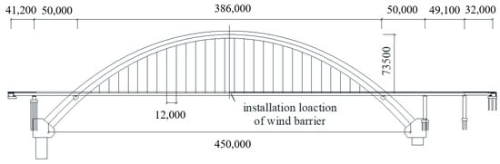
Figure 1.
Schematic drawing of the Xijiang Bridge (unit: mm).
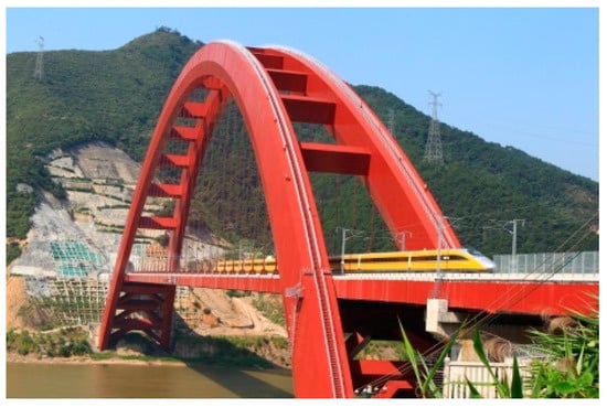
Figure 2.
Photograph of the field test site.
2.2. The Wind Barrier Model and Measurement Points
A ventilating wind barrier is generally adopted in non-wind regions. Holes are distributed evenly on the wind barrier to achieve a certain wind porosity (the proportion of the total areas of holes to the total area of the wind barrier) [16]. The influence of the wind barrier on the train-induced wind load acting on the wind barrier itself mainly includes the height of the wind barrier, the wind porosity, and the shape of the holes. Since the aerodynamic characteristics of a train subject to crosswind depend not only on the shapes of the vehicles, but also the infrastructure and the wind barrier, optimization of the wind porosity, height, and other parameters of the wind barrier is usually conducted to meet the requirements of different wind environments. However, the geometries of the wind barrier are slightly different under different wind environments. The wind porosity of the wind barrier is usually realized through holes or grille bars. However, the holes or grille bars will affect the arrangement of wind pressure measurement points. Thus, the generality of the test results cannot be achieved when considering the wind porosity. Moreover, the test results for the wind barrier without porosity demonstrate an extensive representation because of the largest wind load acting on this type of wind barrier. Therefore, the porosity of the test wind barrier in this paper was set to be 0%, and the height of the wind barrier was set to be 3.0 m, referring to the suggested height in existing literature for the sake of the generality of the test results [27]. In order to eliminate the end effect, the wind barrier model consisted of two compensation segments (the length of each segment was 3 m) and a test segment (the length was 0.2 m). The test segment was located between the two compensation segments. The compensation segments were made of wood boards, and the test segment was made of plexiglass. As shown in Figure 3, the distance between the installed wind barrier and the train was 1.8 m. Considering the side of the wind barrier near the train will experience the majority of the wind loads, only this side of the wind barrier was selected for wind pressure measurements. There was a total of 10 measure points, as illustrated in Figure 3. The interval between each measuring point was approximately 30 cm. It should be noted that measuring point 9 was parallel to the rail surface in Figure 3. The pressure measurement method was adopted to acquire the wind loads acting on the wind barrier.
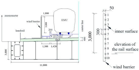
Figure 3.
Locations of the wind barrier and test points (unit: mm).
2.3. Data Acquisition System
The wind pressure acting on the surface of the wind barrier was passed to a pressure scanning value through a Polyvinyl chloride piezometric tube using a high-frequency pressure-scanning valve from Scanivalve. Then, data acquisition and preservation could be realized by a data acquisition system. However, fluctuating wind pressure may be distorted in transforming the wind pressure of the wind barrier’s surface to the pressure-scanning valve because of changes in the amplitude and the phase lag. Therefore, the length of the pipeline used for transferring the pressure should be short, as to ensure the most accurate test results. This indicates that the data acquisition system should be placed near the wind barrier. However, no one is permitted to operate the data acquisition system on the bridge during the whole period of railway operation, according to the regulations of the high-speed railway department. Once the data acquisition parameters are set up for a railway service suspension period, continuous sampling should be started and run for 24 h until turning off at the next service suspension period. A large amount of unnecessary data is saved on the computer, which results in a waste of computer resources. Moreover, in the study, the acquisition parameters were adjusted to fit the changes of the external environment, and zero drift seemed to be impossible. Therefore, a remote-control method was developed to control the data acquisition system located on the bridge, as illustrated in Figure 4. The remote-control method can acquire data and preserve it on the terminal PC through wireless transmission. In addition, a special data processing program was compiled to obtain the loads of the wind barrier from the pressure data and adjust the data acquisition parameters in real time through determining the reliability of data. This remote-control method can not only satisfy the regulations of the high-speed railway department, but it also saves manual duty on the test field.
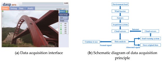
Figure 4.
Remote control data acquisition system.
The Scanivalve pressure scanner used in this test measures differential pressure. A DTC net electronic type pressure scanning system (Pressure Systems, Inc., Hampton, VA, USA) was employed to measure the wind pressure. Its test range is 1 psi, and it is one of the most precise integrated pressure measuring systems in the world (the precision in each wind tunnel test can reach 0.05%). In this study, one module was used to simultaneously monitor a total of 64 pressure measuring points. The sampling frequency was 625 Hz. In order to ensure the accuracy of the test, a stable and reliable reference pressure should be provided. However, atmospheric pressure at the field test site cannot maintain a stable state under the influences of the train-induced wind and the ever-changing natural wind. Thus, the air pressure in a sealed glass bottle (the same as the ambient pressure) was adopted to be the reference pressure. Furthermore, the bottle was soaked in a thermal insulation bucket with ice water to reduce the influence of the ambient temperature on the pressure in the glass bottle [28]. Actually, the measured wind loads on the wind barrier resulted from the interaction of the train-induced wind and the natural wind. In order to analyze the relationship between the running speed of the train and the train-induced wind load on the wind barrier, the intensity of natural wind should be accurately determined. Therefore, anemoscopes were installed on both sides of the upper and lower reaches of the bridge deck in the mid-span. Although the speed of the CRH380A EMU train can be controlled, a video monitoring system was also installed at both ends of the bridge to accurately determine the train’s speed. Moreover, the video monitoring system can provide a reference for the start and end of data acquisition.
3. Data Processing Method
3.1. Inversion Correction of Distorted Fluctuating Wind Pressure
The average wind pressure can be considered as static pressure when the wind pressure of the structural surface is transmitted from the piezometer to the sensor. The amplitude remains the same in such a transmission process. However, the amplitude of fluctuating wind pressure may be reduced due to the friction resistance of the air in the test pipe. In contrast, the resonance of the air in the test pipe, generated by the fluctuating frequency of the pressure signal, can increase the amplitude of the wind pressure. In addition, a certain length of a pressure test pipe will lead to a phase lag [29]. As a consequence of these, the signal measured by the sensor was distorted due to the change in amplitude and the phase lag in the transmission process. In order to ensure the accuracy of the pulsating wind pressure, an inversion correction method was used to amend the measured signal. The inversion correction method could be expressed as follows:
where refers to a Fourier transform of the real wind pressure on the structure’s surface, x(t), Y(ω) refers to a Fourier transform of the pressure signal, y(t), measured by the pressure sensor, and H(ω) is the frequency response function for the pipeline system. The frequency response function, , is a complex function that includes amplitude and phase, which can be obtained through experimental or theoretical calculations. Therefore, both the amplitude and phase of the wind pressure could be corrected through this inverse correction method. It should be noted that the frequency response function of the pipeline system is one of the most significant factors for the inversion correction of distorted fluctuating wind pressure. Thus, the frequency response function of the tubing system was measured before its application in field tests. The detailed description can be found in Reference [29].
3.2. Wavelet Analysis
Wavelet transform (WT) has been widely applied as an excellent time-frequency tool to analyze non-stationary signals in many research aspects over the last decades. The WT can describe the signal time and frequency domain of the local characteristics. It is, therefore, an effective multi-resolution analysis method to identify wind pressure characteristics. WT can divide a signal into the low frequency component and the high-frequency component. This decomposition process can be iterated on the low-frequency component. Therefore, the original signal is decomposed into several levels of lower-resolution components. The reconstructed signal can possess the time characteristics of the original signal, and it can be used to filter the frequency distribution of the signal. By supposing (where represents the Hilbert measurement space), the Fourier transform of , represented by ’, meets the wavelet admissible condition as follows:
where is the mother wavelet, R represents set of reals, and represents the angular frequency. By extending and translating the mother wavelet, a wavelet family can be obtained as follows:
where a is the scale factor and b is the translation factor.
For any function, , the continuous wavelet transform of , can be defined as follows:
Actually, the continuous wavelet transform is highly redundant because of the continuous variation of the scale factor, a, and the translation factor, b. In practice, the scale factor, a, and translation factor, b, are usually discretized in order to improve computation efficiency. Therefore, the measurement is called a discretized wavelet transform and it can be described as follows:
In the present study, the Db4 wavelet was selected for the discretized wavelet transform, which was adopted by Yang et al. [30] to analyze aerodynamic loads on an overhead bridge due to the passage of high-speed trains. On the basis of binary sampling of the wavelet transform at all levels, the time history of the wind pressure can be decomposed to 13 stages. After the reconfiguration of scale factors and wavelet coefficients at different decomposition stages, the low-frequency part, aj (approximate part), and the high-frequency part, dj (detail part), of the original time-varying wind pressure at different scales could be obtained, as shown in Figure 5. The sampling frequency adopted in the process was FS = 625 Hz. According to the Nyquist sampling theorem, the maximum frequency of the original wind pressure signal was FS/2 = 312.5 Hz. The frequency band limits of the low- frequency parts and high-frequency parts at different scales were : (0, 2−(j + 1)FS) and : (2−(j + 1)FS, 2−jFS) ( refers to the decomposition stage). The initial measured wind pressure at each point is defined to be zero before applying the wavelet transform. Therefore, the characteristics of train-induced wind pressure on the wind barrier’s surface can be achieved through analyzing the results directly. This also indicates that the initial measured wind pressure at each point represents the natural wind before the train reaches the measurement site.
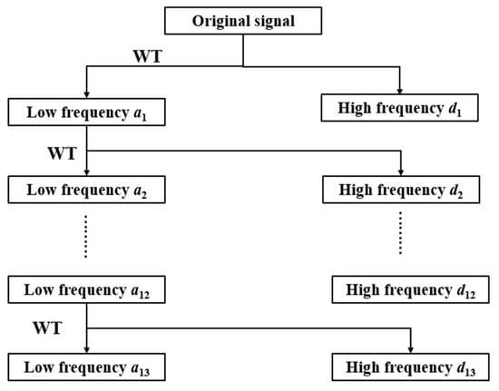
Figure 5.
Schematic diagram of the wavelet transform (WT) decomposition process.
4. Results and Discussion
4.1. Measurement Data
The original measurement data includes both the train-induced fluctuating pressure and the environmental wind pressure. However, the effects of environmental wind on the fluctuating pressure on the barrier can be ignored when the its speed is below 2 m/s [25]. Therefore, the test results presented in this study were selected to satisfy such environmental wind speeds during the passage of the high-speed trains. The wind pressures of three measurement points (point 2, point 7, and point 9) under train-induced wind, with a running speed of 275 km/h, are illustrated in Figure 6. It can be seen from Figure 6 that the variations in wind pressure at each measurement point were basically the same when the high-speed train passed the wind barrier. The pressure variation induced by the slipstream of the high-speed train was dynamically processed in the time domain. The positive value (push effect) during the passage of the head vehicle, and the negative value (pull effect) during the passage of the tail vehicle could be observed, and were similar to the results in References [25,31]. The pressure caused by train-induced wind could be preliminarily divided into three sections, as shown in Figure 6. Section 1 was mainly influenced by the “head wave effect”. The positive wind pressure reached the maximum value when the head vehicle was closest to the test point. This was because of train-induced positive wind pressure acting on the inner surface of the barrier. The positive peak occurred at the arrival of the train noise. Then, the wind pressure dropped to a negative value instantaneously when the head vehicle passed the test point. Therefore, a complete pressure wave was generated by the head vehicle, namely the “head wave effect”.
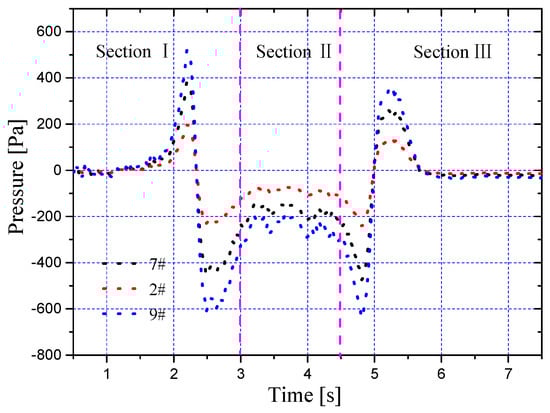
Figure 6.
Measured wind pressure with respect to different test points (train speed = 275 km/h).
Section 2 showed that the negative pressure increased suddenly and then kept a relative steadiness when the middle vehicles passed through the test points. The relative stable performance of pressure in Section 2 was because of the uniform cross section of the train. However, the effect of environment wind, the complex structures of bogies, and inter-carriage gaps resulted in some small fluctuations.
Section 3 was mainly influenced by a “tail wave effect”. The wind pressure dropped to the negative pressure extremum when the tail vehicle was closest to the test point. However, the wind pressure increased instantaneously to the positive pressure extremum after the tail vehicle passed the test point. Thereafter, the pressure dropped to zero. It should be noted that the pressure amplitudes induced by the “head wave effect” were slightly larger than those induced by the “tail wave effect” for each test point. Thus, the train-induced wind generated two impacts with opposite directions on the wind barrier. This can cause oscillations of the wind barrier in the horizontal direction and wave movements in the longitudinal direction (the train’s running orientation).
Pressure amplitude is usually adopted to describe the characteristics of the transient wind load. Figure 7 shows the pressure amplitudes of all points under the train, running at a speed of 275 km/h. It can be seen that the maximum pressure amplitude appeared at point 9. The elevation of point 9 was parallel to the rail surface. Since the top of wind barrier has no boundary condition and the bottom of the wind barrier is mostly sealed to the bridge deck, the pressure amplitude decreased rapidly with an increase in the test point height. The maximum pressure amplitude was about 582 Pa, which is approximately three times that of the minimum pressure amplitude.
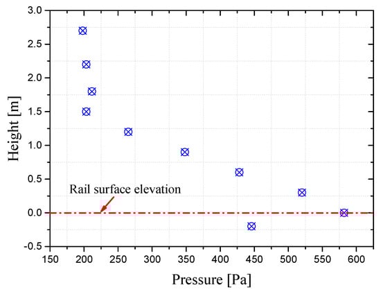
Figure 7.
Peak wind pressure with respect to different heights (train speed = 275 km/h).
Since the peak wind pressure at point 9 was the maximum, the measured data of point 9 was chosen to analyze the relationship between the peak wind pressure and the train speed, as illustrated in Figure 8. It can be observed from Figure 8 that the peak wind pressure was approximately proportional to the square of the running speed of the train. Similar results can be found in previous research regarding scale model studies, numerical investigations, and full-scale tests [23,24,25,26].
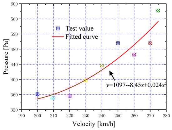
Figure 8.
The peak wind pressures of point 9 under different train speeds.
4.2. Wavelet Transform Analysis
Since the train-induced wind pressure acted on the wind barrier, significant transient and time-varying characteristics were present. Wavelet transform is an effective method to analyze such non-stationary signals. Figure 9 shows the pressure components of some representative decomposition stages after the decomposition and reconfiguration of the original wind pressure. As illustrated in Figure 9, the original wind pressure signal continuously decomposed to a lower frequency level. Each decomposition represents the wind pressure component of different frequency bands. When the decomposition stage was in the low-level range because of the high frequency, it contained a large amount of wind pressure pulsation information at that time. In particular, the reconfiguration curve at the high-frequency part fluctuated quickly. However, the pressure of the high-frequency part basically fluctuated around 0. Therefore, the component of the time-history wind pressure was small in this frequency range. With the increase in the decomposition stage, the frequency range decreased, and the information of wind pressure pulsation gradually disappeared. The pressure signal also smoothened. The wind pressure component in the relatively low-frequency part gradually decreased, and the wind pressure component in the relatively high-frequency part increased slowly. When the composition stage reached level 8, the extreme value of the high-frequency wind pressure suddenly changed. At this moment, the low-frequency range was (0, 1.22 Hz) and the high-frequency range was (1.22 Hz, 2.44 Hz). The components of wind pressure on both ranges were large. In other words, the upper limit in the frequency distribution of the wind pressure component, which was 2.44 Hz, was reached at this time. To further explore the lower limit of the component frequency distribution, the decomposition was performed continuously until level 10. The wind pressure in the low-frequency range, (0, 0.31 Hz), was basically maintained at around 0. The wind pressure in the high-frequency range, (0.31 Hz, 0.62 Hz), reduced sharply. These results indicate that the wind pressure component reached the lower limit of the frequency. At this moment, the frequency was 0.31 Hz. Moreover, the low-frequency part in each decomposition level, shown in the left section of Figure 9, shows that the average wind pressure varied with time. This was because the pressure began to increase in the period of time before the head vehicle reached the measurement points. When the nose of the train was close to the test point, the pressure increased quickly and reached the positive pressure extreme. When the train passed by the test point, the pressure dropped to the negative pressure extremum instantaneously. However, once the train passed by, the negative pressure increased immediately and was steadily maintained. When the end point of the train was close to the test point, the pressure dropped to the negative pressure extremum. However, after the tail of the train passed by the test point, the pressure increased instantaneously to the positive pressure extremum. The signal disappeared gradually after it fluctuated slightly. The time interval between the positive and negative pressure extremes was approximately 0.2 s.
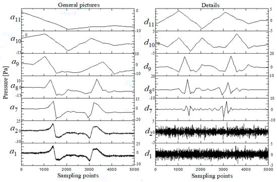
Figure 9.
Wind pressure components of different decomposition layers.
The extreme values of the wind pressure of the transient pressure wave are an important indicator of the size of the pressure component. Figure 10 shows a histogram of the extreme wind pressures of different composition layers over time for the low-frequency and high-frequency parts. The combination of the top seven pressure extreme values in the low-frequency decomposition layer are shown in Figure 10a. The change in the high-frequency information of the same decomposition layer is illustrated in Figure 10b. It can be seen from Figure 10 that the frequency range of the wind pressure was mostly distributed in the low-frequency part. However, the wind pressure extreme values in the low- and high-frequency parts in the eighth decomposition layer were obvious. Specifically, the wind pressure extreme value in the high-frequency part increased by 485%. Therefore, most of the wind pressure information was in this frequency range and continued to level 10. The low-frequency wind pressure extreme value sharply reduced by 70%. This result indicates that the later decomposition levels contain extremely small amounts of wind pressure information. Therefore, most of the wind pressure information was in the low-frequency range (0, 2.44 Hz), especially in the frequency range (0.31 Hz, 2.44 Hz). At the same time, the transient pressure wave under the action of the train-induced wind was dominated by the influence of the time history of the wind pressure in the low-frequency range. It means that the pressure extreme value generated from the train-induced wind on the surface of the wind barrier was significantly influenced by the change in the average wind speed.
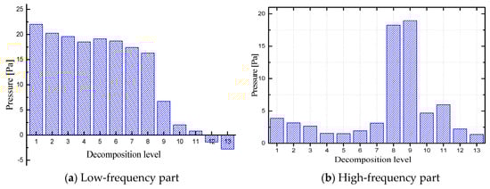
Figure 10.
Extreme pressures of different decomposition layers.
Figure 11 presents a comparison of the wind pressure extremes at different scales through the decomposition and reconfiguration of the wind pressure time history at test point 9 at different running speeds. It can be seen from Figure 10 that the components of the wind pressure at different train speeds were basically consistent in the frequency distribution at different scales. The cut-off points were at the decomposition levels 8, 9, and 10. This indicates that the components of the wind pressure were mostly in the low-frequency range (0.31 Hz, 2.44 Hz). Therefore, the running speed of the train cannot change the wind field characteristics of the train-induced wind, nor the distribution of the wind pressure component in the frequency domain; it can only change the extreme value of the wind pressure. The influence of the average wind over time still dominates the time history information of the wind pressure.
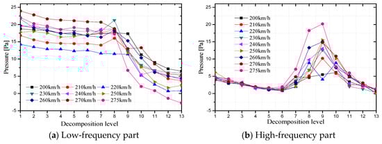
Figure 11.
Comparison of extreme pressures of different decomposition layers under different running speeds.
Figure 12 shows a power spectrum of the wind pressure at test point 9 to further ensure the distribution characteristics of the fluctuating wind pressure energy of the wind barrier in the frequency domain. As shown in Figure 12, the first six peak values in the power spectrum appeared at 0.61, 0.92, 1.37, 1.68, 2.14, and 2.44 Hz, respectively. Thereafter, the power spectrum dropped sharply and tended to be zero. This indicated that the pressure wave energy was mainly distributed in the low-frequency range (0, 2.44 Hz). Figure 13 shows the percentage of low-frequency energy (below 2.44 Hz) in the total energy at point 9 under different train speeds. The proportion of low-frequency energy slightly increased with the increase in train speed. The proportion of total energy to the low-frequency energy on the surface of the wind barrier under the action of the train-induced wind at different speeds was more than 94%. This result further verifies the distribution of wind pressure frequency from the angle of the energy.
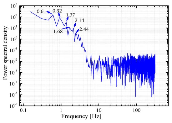
Figure 12.
The power spectrum of wind pressure at test point 9.
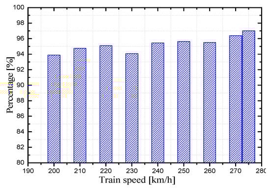
Figure 13.
Percentage of low-frequency energy in total energy.
5. Conclusions
Field measurements were conducted on the Nanning-Guangzhou high-speed railway in order to obtain the high-speed train-induced wind pressure data for wind barriers installed on the Xijiang Bridge. The speed of the CRH380A EMU high-speed train was in the range of 200 km/h–280 km/h. A DTC net electronic type pressure scanning system was used in field measurements. The measured time history curves of fluctuating pressure were analyzed by the wavelet transform signal processing method in order to identify the pressure distribution in different frequency bands. Results showed that the wind pressure on wind barriers caused by train-induced wind had two significant impacts with opposite directions, which were the “head wave” and “tail wave”. Similar results can be found in previous research regarding scale model studies, numerical investigations, and full-scale tests. The peak wind pressure on the wind barrier was approximately proportional to the square of the running speed, and it rapidly decreased with height. The maximum wind pressure occurred at the rail surface height. Furthermore, the fluctuating wind pressure energy on the surface of the wind barrier was mainly distributed in the low-frequency range of 0–2.44 Hz, which accounted for 94% of total energy. This indicates that the low-frequency range component of the wind pressure dominates the design of the wind barrier. Since the fundamental frequency of a barrier turned out to be less than 3.0 Hz, the cyclic loads acting on the barriers due to the repeated passage of high-speed trains will lead to the fatigue of barriers. Therefore, the effects of the aerodynamic pressure generated by high-speed trains on the vibration of barriers is a topic worthy of attention. In addition, the running speed of the train did not change the distribution of the wind pressure component of the wind barrier in the frequency domain. While the wind pressure extreme value was slightly increased with the increase in the train’s speed.
Author Contributions
All the authors made significant contributions to the work. Y.Z., Z.F., X.H., and C.C. conceived this study; Y.Z., Z.F., and J.Z. completed the tests and analyzed the data; S.Z., X.H., and C.C. provided advice for the preparation and revision of the paper; Y.Z., Z.F., X.H., and C.C. wrote the paper; J.Z. and S.Z. reviewed the manuscript for scientific contents.
Funding
The authors gratefully acknowledge the support of the National Key R&D Program of China (Project No. 2017YFB1201204), and National Natural Science Foundations of China (Project Nos. 51508580, U1534206 and 51708202). The work presented in this paper was also supported by grants received from the Natural Science Foundations of Hunan Province (Project No. 2016JJ3149).
Conflicts of Interest
The authors declare no conflicts of interest.
References
- Imai, T.; Fujii, T.; Tanemoto, K.; Shimamura, T.; Maeda, T.; Ishida, H.; Hibino, Y. New train regulation method based on wind direction and velocity of natural wind against strong winds. J. Wind Eng. Ind. Aerodyn. 2002, 90, 1601–1610. [Google Scholar] [CrossRef]
- Suzuki, M.; Tanemoto, K.; Maeda, T. Aerodynamic characteristics of train/vehicles under cross winds. J. Wind Eng. Ind. Aerodyn. 2003, 91, 209–218. [Google Scholar] [CrossRef]
- Bocciolone, M.; Cheli, F.; Corradi, R.; Muggiasca, S.; Tomasini, G. Crosswind action on rail vehicles: Wind tunnel experimental analyses. J. Wind Eng. Ind. Aerodyn. 2008, 96, 584–610. [Google Scholar] [CrossRef]
- Baker, C.; Cheli, F.; Orellano, A.; Paradot, N.; Proppe, C.; Rocchi, D. Cross-wind effects on road and rail vehicles. J. Veh. Mech. Mobil. 2009, 47, 983–1022. [Google Scholar] [CrossRef]
- He, X.H.; Wu, T.; Zou, Y.F.; Chen, Y.F.; Guo, H.; Yu, Z.W. Recent developments of high-speed railway bridges in China. Struct. Infrastruct. Eng. 2017, 13, 1584–1595. [Google Scholar] [CrossRef]
- Matschke, G.; Schulte, W.B. Measures and strategies to minimise the effect of strong cross winds on high speed trains. In Proceedings of the World Congress of Railway Research, Florence, Italy, 16–19 November 1997; pp. 178–255. [Google Scholar]
- Raine, J.K.; Stevenson, D.C. Wind protection by model fences in a simulated atmospheric boundary layer. J. Wind Eng. Ind. Aerodyn. 1977, 2, 159–180. [Google Scholar] [CrossRef]
- Coleman, S.A.; Baker, C.J. The reduction of accident risk for high sided road vehicles in cross winds. J. Wind Eng. Ind. Aerodyn. 1992, 41–44, 2685–2695. [Google Scholar] [CrossRef]
- Jiang, C.X.; Liang, X.F. Effect of the vehicle aerodynamic performance caused by the height and position of wind-break wall. China Railw. Sci. 2006, 27, 66–70. (In Chinese) [Google Scholar]
- Liu, Q.K. Study on the system to ensure train operation safety under strong wind. Eng. Mech. 2010, 27, 305–310. (In Chinese) [Google Scholar]
- Kwon, S.D.; Kim, D.H.; Lee, S.H.; Song, H.S. Design criteria of wind barriers for traffic. Part1: Wind barrier performance. Wind Struct. 2011, 14, 55–70. [Google Scholar] [CrossRef]
- Kozmar, H.; Procino, L.; Borsani, A.; Bartoli, G. Sheltering efficiency of wind barriers on bridges. J. Wind Eng. Ind. Aerodyn. 2012, 107–108, 274–284. [Google Scholar] [CrossRef]
- Xiang, H.Y. Protection Effect of Wind Barrier on High Speed Railway and Its Wind Loads. Ph.D. Thesis, Southwest Jiaotong University, Chengdu, China, 2013. [Google Scholar]
- He, X.H.; Zou, Y.F.; Wang, H.F.; Shi, K.; Han, Y. Aerodynamic characteristics of a trailing rail vehicles on viaduct based on still wind tunnel experiments. J. Wind Eng. Ind. Aerodyn. 2014, 135, 22–33. [Google Scholar] [CrossRef]
- He, X.H.; Zou, Y.F.; Du, F.Y. Mechanism analysis of wind barrier’s effects on aerodynamic characteristics of a train on viaduct. J. Vib. Shock 2015, 34, 66–71. (In Chinese) [Google Scholar]
- Consultation Report of the Noise Barriers in Chinese Railway Passenger Dedicated Line; Planning Engineering Consulting + Services China LTD: Beijing, China, 2007. (In Chinese)
- Zhu, Z.Q.; Cheng, Z.Q. Numerical simulation and experimental verification of verification of dynamic pressure on noise barriers of high speed railways. Railw. Stand. Des. 2011, 11, 77–80. (In Chinese) [Google Scholar]
- Jiao, C.Z.; Gao, B.; Wang, G.D. Vibration analysis of noise barrier structures subjected to train induced impulsive wind pressure. J. Southwest Jiaotong Univ. 2007, 42, 531–536. (In Chinese) [Google Scholar]
- Carassale, L.; Brunenghi, M.M. Dynamic response of trackside structures due to the aerodynamic effects produced by passing trains. J. Wind Eng. Ind. Aerodyn. 2013, 123, 317–324. [Google Scholar] [CrossRef]
- Long, L.P.; Zhao, L.B.; Liu, L.D. Research on the air turbulence force loaded on noise barrier caused by train. Eng. Mech. 2010, 27, 246–250. (In Chinese) [Google Scholar]
- Khayrullina, A.; Blocken, B.; Janssen, W.; Straathof, J. CFD simulation of train aerodynamics: Train-induced wind conditions at an underground railroad passenger platform. J. Wind Eng. Ind. Aerodyn. 2015, 139, 100–110. [Google Scholar] [CrossRef]
- Paz, C.; Suarez, E.; Gil, C. Numerical methodology for evaluating the effect of sleepers in the underbody flow of a high-speed train. J. Wind Eng. Ind. Aerodyn. 2017, 167, 140–147. [Google Scholar] [CrossRef]
- Jordan, S.; Johnson, T.; Sterling, M.; Baker, C. Evaluating and modeling the response of an individual to a sudden change in wind speed. Build. Environ. 2008, 43, 1521–1534. [Google Scholar] [CrossRef]
- Tokunaga, M.; Sogabe, M.; Santo, T.; Ono, K. Dynamic response evaluation of tall noise barrier on high speed railway structures. J. Sound Vib. 2016, 366, 293–308. [Google Scholar] [CrossRef]
- Xiong, X.H.; Li, A.H.; Liang, X.F.; Zhang, J. Field study on high-speed train induced fluctuating pressure on a bridge noise barrier. J. Wind Eng. Ind. Aerodyn. 2018, 177, 157–166. [Google Scholar] [CrossRef]
- Vittozzi, A.; Silvestri, G.; Genca, L.; Basili, M. Fluid dynamic interaction between train and noise barriers on High-Speed-Lines. J. Procedia Eng. 2017, 199, 290–295. [Google Scholar] [CrossRef]
- Zhang, J. Wind-tunnel test investigations and analysis on wind break performances of wind fences on railway. J. Railw. Sci. Eng. 2007, 4, 13–17. (In Chinese) [Google Scholar]
- Liang, X.F. Research on test technique to measure air pressure distribution on external surface of real train. J. China Railw. Soc. 2002, 24, 95–98. (In Chinese) [Google Scholar]
- Irwin, H.J.; Cooper, K.R.; Girard, R. Correction of distortion effects caused by tubing systems in measurements of fluctuating pressures. J. Wind Eng. Ind. Aerodyn. 1979, 5, 93–107. [Google Scholar] [CrossRef]
- Yang, N.; Zheng, X.K.; Jian Zhang, J.; Law, S.S.; Yang, Q.S. Experiment and numerical studies on aerodynamic loads on an overhead bridge due to passage of high-speed train. J. Wind Eng. Ind. Aerodyn. 2015, 140, 19–33. [Google Scholar] [CrossRef]
- Hemida, H.; Baker, C.J.; Gao, G. The calculation of train slipstreams using large-eddy simulation. Proc. Inst. Mech. Eng. Part F J. Rail Rapid Transit 2014, 228, 26–36. [Google Scholar] [CrossRef]
© 2019 by the authors. Licensee MDPI, Basel, Switzerland. This article is an open access article distributed under the terms and conditions of the Creative Commons Attribution (CC BY) license (http://creativecommons.org/licenses/by/4.0/).