After presenting the main components and scheme of the 2D control system, this section first analyses the NanoPla dynamic model and then presents a 2D positioning control strategy for the NanoPla. Finally, the NanoPla’s performance is experimentally validated.
3.1. Dynamic Characterisation of the System
In the NanoPla, the motors are placed in parallel pairs (
Figure 3); thus, two motors, motor 1 and motor 2 (represented as M1 and M2 in
Figure 3b), generate forces on the X-axis (F
M1 and F
M2) that move the platform in the X-direction. Similarly, the other two parallel motors, motor 3 and 4 (M3 and M4), generate forces on the Y-axis (F
M3 and F
M4) that move the platform in the Y-direction. In addition, the four motors are placed symmetrically at a distance R (169.9 mm) from the centre of the platform and, thus, their forces generate a torque at the centre of the moving platform, around the Z-axis. The movements of the platform in the X- and Y-axes -X
s and Y
s- and the rotation around Z-axis -θ
zs- are monitored by the 2D laser interferometer system (Laser Y1, Y2, and X). The total forces in the X- and Y-axes and the torque around the Z-axis -T
z- can be calculated as follows:
The dynamic model of a Halbach linear motor working as a positioning actuator in a pneumatically levitated linear stage was identified as a servosystem in a previous work [
14]. In this system, the electromagnetic horizontal force generated by the motor around the stable equilibrium position (F
x = 0, F
z > 0) acts as a proportional controller. The closed-loop transfer function that relates the equilibrium position, X
eq(s), to the position of the stage, X(s), was identified with a spring-mass-damper model (second order system). The NanoPla 2D positioning model is expected to present a similar second-order transfer function in each axis of motion, since it uses the same actuators and the moving platform is also pneumatically levitated. The transfer function of the system can be obtained experimentally, which enables a better understanding of the system and allows tuning of the controllers in advance, which facilitates tasks in the experimental setup.
The force generated by each Halbach motor around the stable equilibrium position (linear zone) can be defined as
where K
M is the slope of the thrust force generated by each Halbach linear motor around the equilibrium position. The forces along the X-axis generated by the parallel motor pair M1 and M2 at the initial position are represented in
Figure 4. The linear zone and the slope around the stable equilibrium position are also represented in
Figure 4. As shown, the linear zone has a length of approximately 5 mm, with the stable equilibrium position in the middle of the region. In this system, the stable equilibrium position of the parallel pair of Halbach linear motors M1 and M2 is set at the same X-coordinate. Thus, the total force, F
x, generated around the stable equilibrium position is twice the force defined in Equation (4). Therefore, the transfer function that relates the final position of the stage X(s) with the defined stable equilibrium position X
eq(s) is the following:
where
m is the mass of the moving part and
bX defines the viscous-friction elements of the setup and the eddy-current damping of the motors in the X-axis. Additionally, 2K
M is the slope of the total thrust force, F
x, generated by the pair of Halbach linear motors around the equilibrium position in the X-axis (
Figure 4). Since the actuator distribution in the moving platform is symmetrical, the same equations are considered valid for the Y-axis. The mass of the moving platform is known (13.25 kg), and the value of K
M depends on the reference value set for the vertical force at the stable equilibrium position, F
zref. This value defines the amplitude of the sinusoidal distribution of the forces along the axis of motion, while the spatial period is defined by the design [
9]. For instance, when F
zref is set to 1 N, K
M is approximately 205 N/m, and when F
zref is set to 2 N, K
M is 410 N/m. Therefore, K
M and
m are known, whereas the viscous-friction factor
bX must be obtained experimentally.
On the other hand, rotation around the Z-axis (θ
z) is generated by torque acting on the central point of the moving platform. This torque (T
z) is the sum of the torques generated by each motor in the plane of motion (
Figure 3b). The 2D plane mirror laser interferometer system requires the rotation of the moving platform to be less than ±1.2 × 10
−4 rad, according to the manufacturer’s specifications, to prevent misalignment between the laser beam and plane mirror. Therefore, to rotate the moving platform by angle Δθ
z, each motor would have to perform a displacement of the same magnitude, equal to Δθ
z·R, in the direction that favours that rotation. According to this, the torque generated by the four motors of the NanoPla to perform a rotation of Δθ
z can be calculated as follows:
It is worth mentioning that the angular position θz is considered to be a stable equilibrium angular position when, at that angular position, the platform remains still and after a disturbance, it comes back to the same angular position. This stable equilibrium position is created when the moving platform is perfectly aligned in the X- and Y-axes—that is, θz,eq = 0. Thus, as in the previous case, the transfer function that relates the final angular position of the stage θz(s) with the defined stable equilibrium angular position θz,eq(s) is defined by Equation (7), where bθ is the damping factor in θz, and Iz is the inertia of the moving platform.
3.2. 2D Control Strategy
The four motors are placed in parallel pairs. Thus, as long as the motor pairs displace the same distance, the moving platform remains aligned. It was experimentally verified that the moving platform can be positioned along its working range by controlling each of the motors individually with a 1D positioning strategy (presented in [
9]) implemented in each motor. Nevertheless, independently controlling each motor results in undesired rotations around the Z-axis during the transient response—that is, when the platform is moving from one position to other. Undesired rotations cause misalignments between the laser beams and plane mirrors, which can affect the performance of the laser system and even impede the displacement measurements. Therefore, in order to prevent undesired rotations of the moving platform during motion, it is necessary to coordinate the control of the four motors in a 2D control strategy.
On the other hand, in [
7], control of the out-of-plane motion was proven to be unnecessary due to the high stiffness of the air bearings. Similarly, in the NanoPla, the moving platform is levitated by three vacuum-preloaded air bearings with an input pressure of 0.41 MPa and an input vacuum of 15 mmHg, as recommended by the manufacturer. At these working conditions, the air bearings have a stiffness of 13 N/µm. As calculated in [
9], the variation of the vertical force during motion has a maximum increment of 7%, which results in negligible vibrations of the moving platform. Therefore, control of the out-of-plane motion in the NanoPla is unnecessary, although it will be monitored by three capacitive sensors.
The proposed control strategy positions the platform in the X- and Y-axes and minimises rotations around the Z-axis (θzref = 0), to prevent laser system misalignments. This is done with three independent proportional-integral-derivative (PID) controllers that act on the forces generated in the X- and Y-axes by the motor pairs (Fx and Fy) and on the torque (Tz) generated by the four motors. The positioning feedback (Xs, Ys, and θs) is provided by the three laser beams (Laser Y1, Y2, and X) of the laser system. Considering the symmetry of the moving platform, the total forces and torque are divided between the four motors, and the horizontal force that each of the motors needs to generate is computed.
Figure 5 illustrates the scheme of the control system that has been implemented in this project. The input of the control system is the target position (X
ref, Y
ref) of the moving platform that is entered in the graphic user interface. In addition, the rotation around the Z-axis should be kept minimal (θ
zref = 0). The previously described control strategy is computed in Simulink
® on the host PC (
Figure 5). Firstly, this strategy calculates the horizontal forces that each of the linear motors needs to generate to correct positioning errors. Then, the phase currents that each linear motor requires to generate those forces are calculated according to the commutation law defined in [
9]. The outputs of the control strategy are the corresponding phase voltages that the control hardware must generate for each motor. These phase voltages are generated at the power stage of each DMC kit. Then, the interaction of the phase currents flowing through the stator coils with the magnetic field of the magnet arrays of the moving platform generates horizontal forces that move the platform. This movement is recorded by the laser system and fed back to the control strategy.
3.3. Experimental Results
The procedure for experimentally obtaining the transfer function in a linear stage was defined in [
14]. This procedure has been adapted to the NanoPla, where a parallel pair (M1 and M2) generates the thrust force in the X-axis, whereas the other parallel pair (M3 and M4) generates the force in the Y-axis (
Figure 3). In order to obtain the transfer function in the X-axis, the motor pairs aligned in the Y-axis are set to remain still at the initial position in the Y-axis (Y
ref = 0, θ
z,ref = 0), acting as a guiding system that prevents the movement of the moving platform on the Y-axis and its rotation around the Z-axis. Then, the NanoPla is displaced from its initial position inside the linear zone by using the electromagnetic force of the motor pair aligned on the X-axis (M1 and M2). The movement of the moving platform is recorded by the laser system, and then the spring mass damper model of Equation (5) is fit to the response. The same procedure is followed to obtain the transfer function on the Y-axis.
Figure 6 represents the experimentally obtained 1 mm step response of the stage on the X- and Y-axes (X
s and Y
s) when F
zref is set to 2 N. The simulated response of the adjusted model is also shown (X
sim and Y
sim). The obtained values for
m and K
M match the actual mass of the moving platform and the slope of the thrust force around the stable equilibrium position, respectively. The viscous-friction elements (
b) have a value of 56.8 N·s/m on the X-axis and for 63.07 N·s/m on the Y-axis. The differences between axes could be due to geometrical errors in assembly and the fact that the moving platform is not perfectly symmetrical due to the presence of the plane mirrors, which are larger for the dual beam Y-axis. In addition, it was experimentally verified that by varying F
zref, the value of K
M changed as expected, and the values of
m and
b remained invariable.
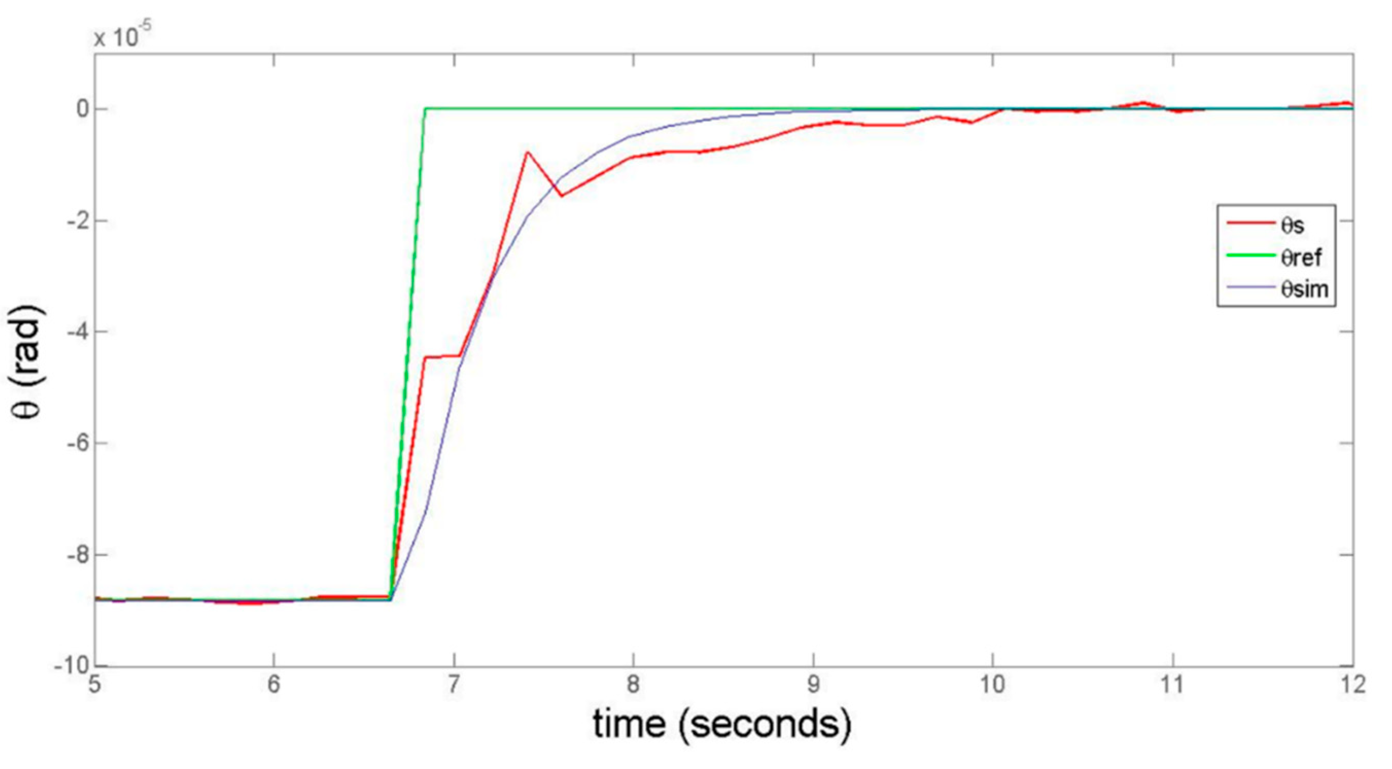
In order to obtain the transfer function for the rotation around the Z-axis, the four motors are set to displace from an initial rotated position to a stable equilibrium position θ
z,eq = 0. At this initial position, the angular deviation is not null. In order to define the initial position, the four motors are displaced at a distance of Δθ
z·R, equal to 15 µm. In each motor pair, each motor displaces in an opposite direction to contribute to the rotation around the central point of the stage, generating an angular deviation of 8.83 × 10
−5 rad, which is close to the maximum displacement allowed without losing the laser system’s alignment. The experimentally obtained values for I
z and K
M approximately match the actual inertia of the moving platform and the slope of the thrust force around the stable equilibrium position, respectively. Nevertheless, due to the limited range of the angular deviation and the short response time, the recorded response is not smooth enough to perfectly match the simulated plant.
Figure 7 represents the experimentally obtained 8.83 × 10
−5 rad step response of the stage around the Z-axis (θ
s). The simulated response of the adjusted model is also shown (θ
sim).
After the transfer function identification, the proposed control system was implemented in the NanoPla, and its correct performance was experimentally verified. For these experiments, the vertical force generated by each motor was defined as 2 N, which limits the phase currents’ working range to ±0.83 A.
Firstly, the stability of the positioning control system was examined for a long period of time. The moving platform was set to remain still at the initial position for 30 min, and it was experimentally verified that the position deviations are confined to ±1 µm. In
Figure 8, a 400 s period of this test is shown, and the root mean square (RMS) deviation during this time is 0.28 µm. The results in the Y-axis are similar, since the moving platform is symmetrical. During this period of time, the force generated by each linear motor varied between ±2 mN—that is, the system worked around the stable equilibrium position, as expected.
As mentioned earlier, the NanoPla has a two-stage scheme. The moving platform performs coarse movement in a large working range of 50 mm × 50 mm. Once the moving platform arrives at the target position, it stays static (air bearings off), and a piezo-nanopositioning stage placed on the inferior base performs the fine displacement required for the scanning task. The selected commercial piezostage has a working range of 100 µm × 100 µm in the XY-plane. Therefore, as mentioned, it is defined as a requirement that the position control system has a positioning error smaller than 10 μm, so this error can be corrected by the fine motion of the piezo stage.
Therefore, the performance of the control system was tested when performing a displacement to the target position. Then, 10 μm step responses were taken in the X- and Y-directions. At the same time, the perturbation to the other axis was also recorded, as shown in
Figure 9. The perturbed motions in the other axis demonstrate that there is a dynamic coupling between axes. This is unavoidable because there is only one moving part that is affected by the vibrations of the four motors. This perturbation generates a displacement on the Y-axis of a maximum of 2 µm during the transient response. Nevertheless, once the NanoPla achieves its target position on the X-axis, the positioning error on the Y-axis is corrected. In addition, it has been observed that during the transient response, the maximum angular deviation is 1.5 × 10
−5 rad, which is inside the tolerance of ±1.2 × 10
−4 rad required for the laser system to read.
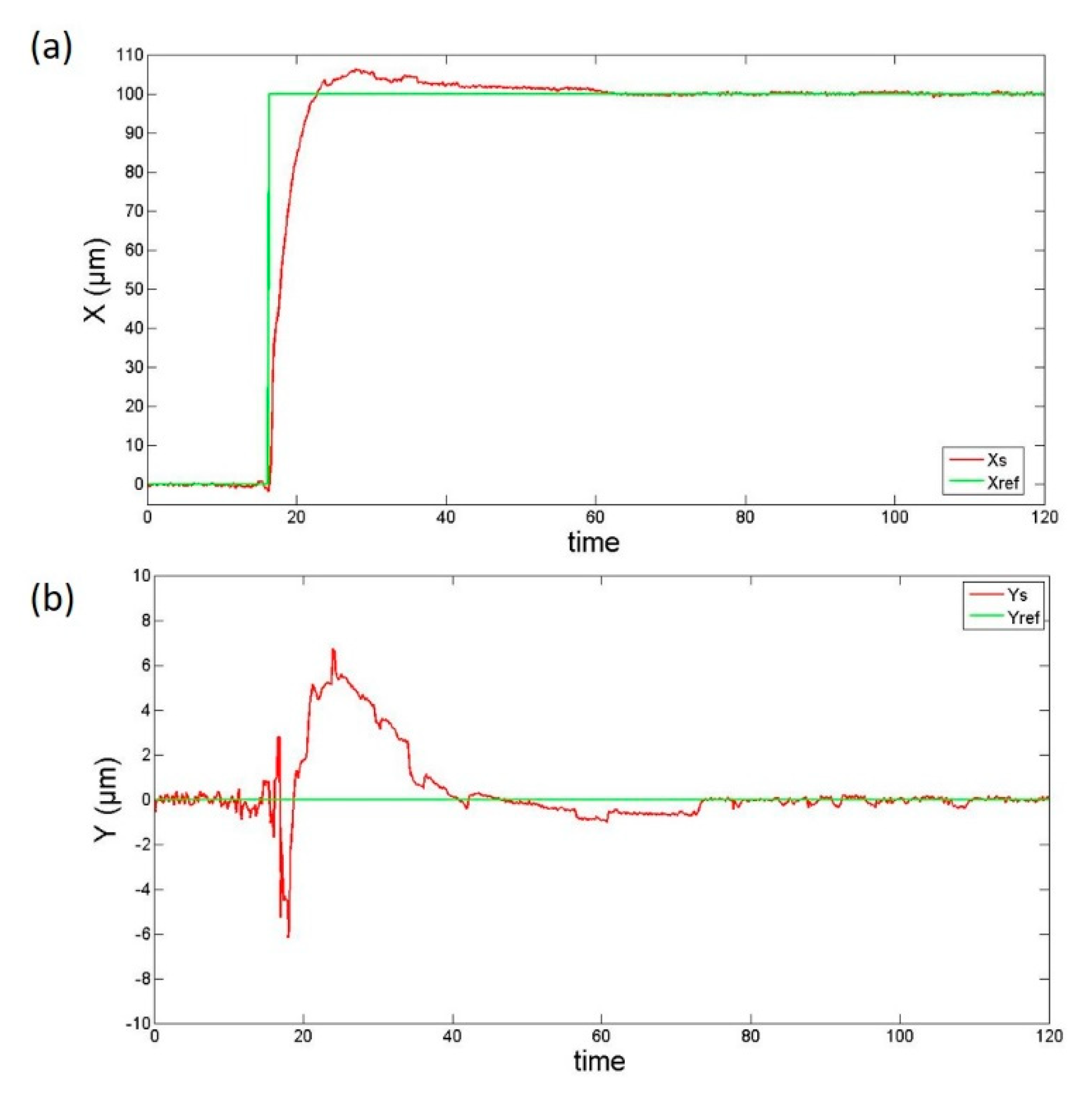
Similarly, 100 μm step responses were taken in the X- and Y-directions, while the perturbation to the other axes was also recorded, as shown in
Figure 10.
As in the previous case, the displacement in one axis generates perturbations in the other axis. This perturbation generates a displacement of a maximum of 7 µm on the Y-axis during the transient response, which is corrected when the NanoPla achieves its stationary state. In addition, it has been observed that during the transient response, the maximum angular deviation is 7.3 × 10⁻⁵ rad, which is inside the tolerance of ±1.2 × 10⁻⁴ rad required for the laser system to read.
It should be taken into account that the transient response can be adjusted depending on the requirements of the application by changing the parameters of the PID controller.
On the other hand, planar scanning motion is the typical motion used in precision engineering such as nanomanufacturing and metrological characterisation. Several experimental results are presented to demonstrate the scanning capability of the developed positioning control system.
Figure 11a shows a displacement on the X-axis of the moving platform from the centre to one extreme of the working range at a constant speed. Similarly,
Figure 11b shows a 1 mm forward and backward displacement on the Y-axis.
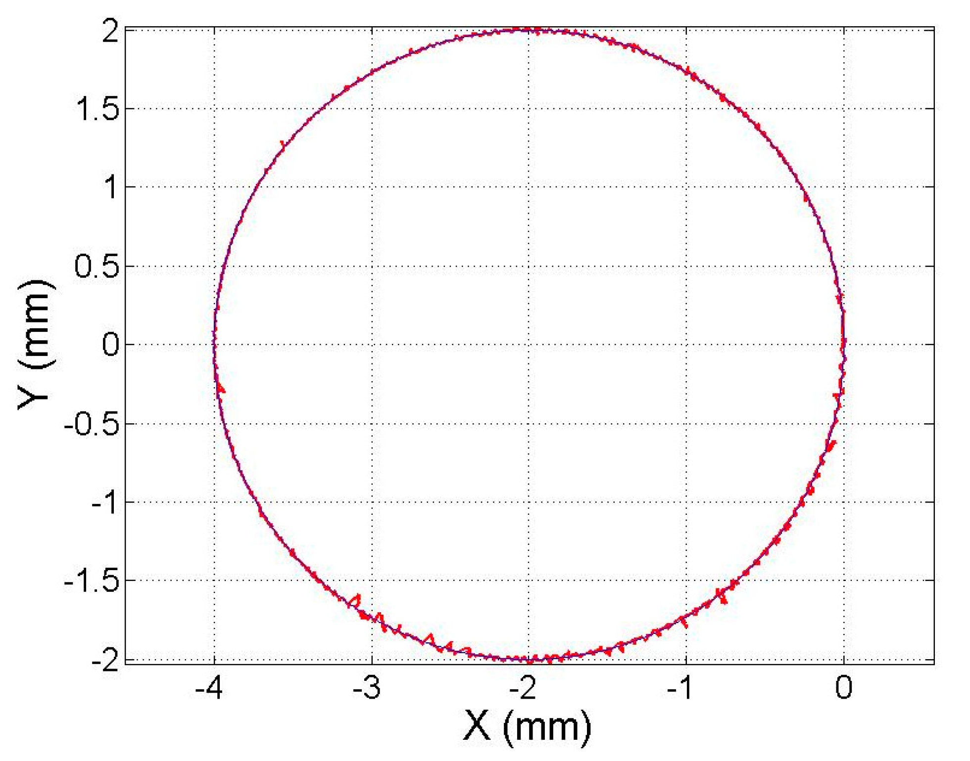
In addition, it has been verified that the platform can perform simultaneous movement on the X- and Y-axes without losing the alignment between the laser beam and plane mirrors.
Figure 12 illustrates the circular motion performed simultaneously on the X- and Y-axes.


