A Tweak-Cube Color Image Encryption Scheme Jointly Manipulated by Chaos and Hyper-Chaos

Featured Application

Since the proposed scheme can efficiently perform image encryption, it can be applied to real-time communication, such as telemedicine.

Abstract

This paper proposes a novel tweak-cube color image encryption scheme jointly manipulated by chaos and hyper-chaos. One-dimensional (1D) chaotic maps are effortless to operate, but the key space is relatively small. The hyperchaotic system has complex dynamics properties, which are capable of compensating for the defects of 1D chaotic maps. Thus, we first raise an improved 1D chaotic map with an increased key space. Then, we associate it with a four-dimensional (4D) hyperchaotic system to generate the key streams and further rotate and shift the rows and columns of each component of Red (R), Green (G), and Blue (B) for the color image. The permuting mode is to disturb the original position of the pixels by mimicking the way of twisting the Rubik’s cube. Moreover, the key stream updated by the plain images is also utilized for diffusion and scramble at the bit level. As a consequence, our cryptosystem enhances the security without at the expense of increasing time cost.

1. Introduction

Digital image is one of the most popular multimedia forms at present, and it is widely used in politics, economy, national defense, and education. Since images contain a lot of information, we must worry about data being leaked, falsified, and counterfeited. Image encryption is a very effective means of protecting images by processing them into an unrecognizable form. Moreover, image data has its own unique properties: large amount of data, high redundancy, and strong correlation between adjacent pixels [1]. These features make the traditional encryption algorithms such as data encryption standard (DES), advanced encryption standard (AES), and Rivest-Shamir-Adleman (RSA) unsatisfactory. Thus, plenty of new encryption methods have been developed based on various technologies, such as chaos [2,3,4,5], compressed sensing [6,7], wave transmission [8,9], hash function [10,11], deoxyribonucleic acid coding [12,13], genetics [14], gray code [15], elliptical curve [16], and so on. Among them, the chaos-based image encryption schemes have received extensive attention due to the advantages of chaotic systems. They are ergodic, dispersive, and highly sensitive to initial conditions.

In comparison with the methods of encrypting with multidimensional (MD) chaotic maps, the design of cryptosystems with one-dimensional (1D) chaotic maps has the superiorities of simple structures and commodious operations. The most frequently utilized is the Logistic map. At the outset, Pareek et al. employed two Logistic maps to control the tracks of image pixels for encryption [17]. Singh et al. proposed an encryption method that combines the Logistic map and Hartley transform to improve robustness [18]. Then, Wang et al. applied the Logistic map to encrypt the R, G, B components of a color image at the same time and make these components affect each other [19]. Nonetheless, the Logistic map still has several defects: the chaos region is small, the output sequences are uneven, and the dynamic characteristics are not complicated enough. As a consequence, some researchers have ameliorated the Logistic map to design algorithms. Wu et al. presented a cryptosystem with a two-dimensional (2D) Logistic map of complicated basin structures and attractors [20]. Zhou et al. combined the Logistic map with another two existing 1D maps to raise a novel chaotic system for image encryption [21], and Hua et al. also introduced a new 2D Sine Logistic modulation map (2D-SLMM) to change the image pixel positions [22]. Even recently, some scholars yet have been hammering at encryptions with Logistic map transformation. Pak et al. adopted a linear–nonlinear–linear theory to shuffle plain images [23]. Hanis et al. put forward a novel butterfly-like structure algorithm by using the improved Logistic map [24].

Considering that the above techniques have insufficient finite parameter space to resist brute force attacks and are not conducive to real-time communication, the contributions we have made are summarized as follows. (1) We propose a novel 1D chaotic map with larger key space and better chaotic properties. Simultaneously, it is combined with a 4D hyperchaotic map to control the generation of the key streams, which makes the randomness more superior. (2) We excogitate a color image encryption scheme that mimics the Rubik’s cube motion, which can be effectively used for real-time communication and authentication without compromising time cost and safety quality. Moreover, due to our scheme can scramble images by rotating and shifting them at the pixel-level and bit-level promptly, it is suitable as a secure transmission mode in telemedicine systems. The rest of this paper is organized as follows. Section 2 introduces the modified 1D chaotic map and hyperchaotic system. Section 3 presents our cryptosystem. Section 4 gives simulation results. Section 5 evaluates the security performance. And the final section draws a conclusion.

2. Preliminaries

2.1. The Logistic-Fraction Hybrid Chaotic Map

In this section, a new chaotic map called the Logistic-Fraction hybrid chaotic map (LFHCM) is recommended, which is defined as Equation (1). The LFHCM is derived from the classical Logistic map and Fraction map [25], and they can be mathematically represented as Formulas (2) and (3).

$${\mathrm{x}}_{\mathrm{k}+1}=\mathrm{L}({\mathrm{x}}_{\mathrm{k}})=\mathrm{a}{\mathrm{x}}_{\mathrm{k}}{(1-{\mathrm{x}}_{\mathrm{k}})}^2\times \frac{1}{{\mathrm{x}}_{\mathrm{k}}^2+1}$$

(1)

$${\mathrm{y}}_{\mathrm{k}+1}=\mathrm{L}({\mathrm{y}}_{\mathrm{k}})=\mathrm{b}{\mathrm{y}}_{\mathrm{k}}(1-{\mathrm{y}}_{\mathrm{k}})$$

(2)

$${\mathrm{z}}_{\mathrm{k}+1}=\mathrm{F}({\mathrm{z}}_{\mathrm{k}})=\frac{1}{{\mathrm{z}}_{\mathrm{k}}^2+0.1}-\mathrm{c}{\mathrm{z}}_{\mathrm{k}}$$

(3)

where control numbers $\mathrm{a}\in [0,11.5]$ $\mathrm{b}\in [0,4]$, and $\mathrm{c}\in [0,1]$. In addition, the output ranges of the three maps are also different, ${\mathrm{x}}_{\mathrm{k}}\in [0,1.56]$, ${\mathrm{y}}_{\mathrm{k}}\in (0,1)$, and ${\mathrm{z}}_{\mathrm{k}}\in [-10.0025,10.0025]$. Then, the analytical tests can verify that the LFHCM has more complex dynamic characteristics.

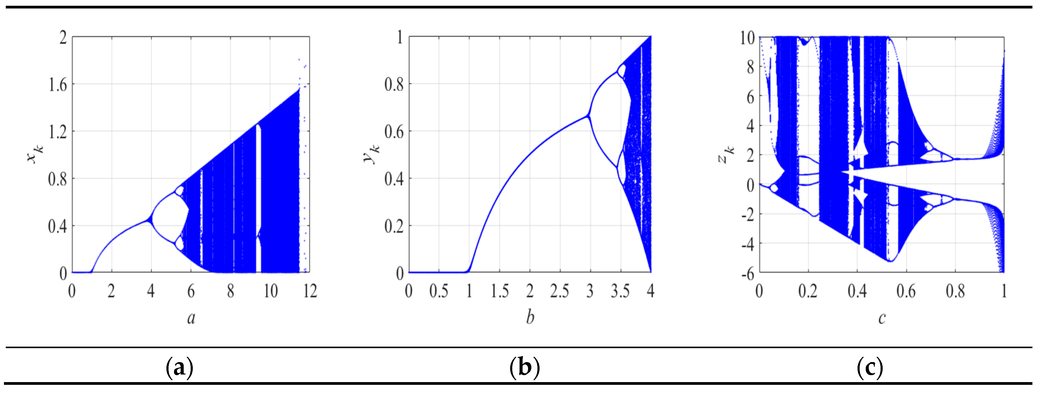
2.1.1. Bifurcation Graph

The bifurcation graph can objectively reflect the region and state of the chaotic behavior of a map. Figure 1 exhibits the bifuration graphs of the LFHCM, Logistic map, and Fraction map. It can be found that the Logistic map shows chaotic characteristics only when $\mathrm{b}\in (3.6,4]$. Although the Fraction map has more complex dynamic properties than the Logistic map, its chaotic interval length is also less than 1. The interval in which the LFHCM presents chaotic state is $\mathrm{a}\in [5.9,11.5]$. It is obvious that the chaotic region of the new chaotic map is increased, which means that the key space is also improved. Besides, in contrast to the intervals of some 1D chaotic maps in

Table 1. Comparison of chaotic intervals between the LFHCM and other one-dimensional (1D) chaotic maps.

Chaotic Maps	Chaotic Regions
The LFHCM	$[5.9,11.5]$
The Logistic map	$(3.6,4]$
The Fraction map	$[0.07,0.15]\cup [0.25,052]\cup [0.57,0.68]$
Modified logistic map in [24]	$[3.9,6.27]$
Sine-Tent systemin [26]	$[0,4]$

, the LFHCM has the largest region.

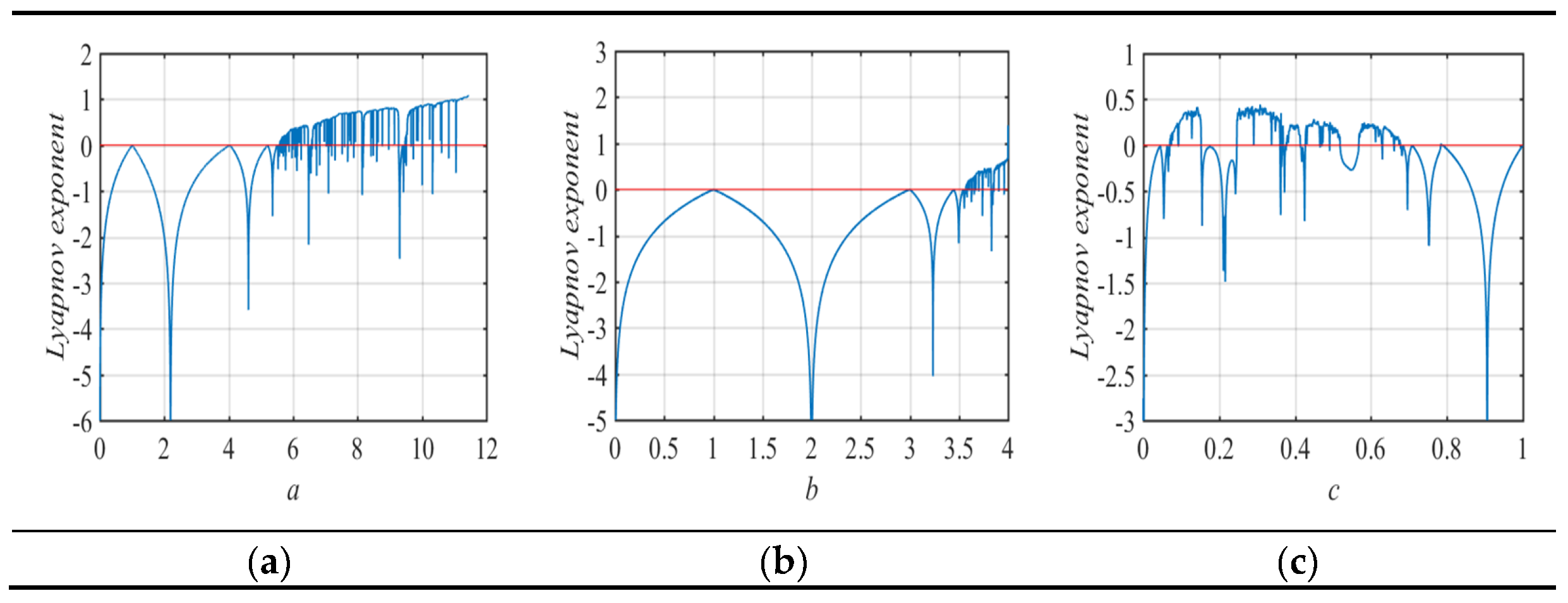
2.1.2. Lyapunov Exponent

The Lyapunov exponent is used to characterize the motion of a system. When it is calculated as a positive number, it indicates that a map has chaotic behavior. Not only that, the larger the Lyapunov exponent, the better the chaotic properties of the map. Besides, the definition of the Lyapunov exponent for a 1D chaotic map ${\mathrm{x}}_{\mathrm{k}+1}=\mathrm{F}({\mathrm{x}}_{\mathrm{k}})$ is as follows:

$$\mathsf{\lambda }({\mathrm{x}}_0)=\underset{\mathrm{n}\to \infty }{\lim }\left\{\frac{1}{\mathrm{n}}{\displaystyle \sum _{\mathrm{k}=0}^{\mathrm{n}-1}\ln }\left|{\mathrm{F}}^{\prime }({\mathrm{x}}_{\mathrm{k}})\right|\right\}$$

(4)

Since the Lyapunov exponent $\mathsf{\lambda }$ is independent of the initial value ${\mathrm{x}}_0$, we arbitrarily chose ${\mathrm{x}}_0=0.5$. Moreover, in order to observe the change between the adjacent iteration points as a whole, the number of iterations $\mathrm{n}$ should be chosen as large as possible, so we set $\mathrm{n}=20,000$. Then, calculated the derivatives of the LFHCM, Logistic map, and Fraction map according to Equations (1)–(3), and substituted the results into Equation (4) to get the Lyapunov exponent plots exhibited in Figure 2. It can be seen that the LFHCM has larger Lyapunov exponents than the other two maps, which means that its orbit is rapidly separated in the direction of the positive Lyapunov exponent and it is sensitive to initial values.

2.1.3. Approximate Entropy

Approximate entropy (ApEn) is a nonlinear dynamic parameter used to quantify the regularity and unpredictability of time series fluctuations [27]. It can also measure the complexity of a chaotic map. Moreover, the larger the calculated ApEn value, the more complicated the sequence generated by the chaotic map is. We set the control parameters 11.44, 3.99, and 0.31 for the LFHCM, Logistic map, and Fraction map separately. Then, we calculated the ApEn of the three maps with different thresholds, as shown in

Table 2. Approximate entropy (ApEn) values of 1D chaotic maps.

Chaotic Maps	Thresholds
	0.02	0.04	0.06	0.08	0.10	0.12	0.14	0.16	0.18	0.20	0.22	0.24	0.26
The LFHCM	0.36	0.55	0.66	0.71	0.75	0.76	0.81	0.82	0.84	0.85	0.84	0.86	0.85
The Logistic map	0.35	0.47	0.53	0.53	0.55	0.56	0.57	0.59	0.27	0.56	0.54	0.53	0.54
The Fraction map	0.15	0.23	0.28	0.33	0.37	0.38	0.41	0.42	0.45	0.47	0.46	0.47	0.46

. It can be seen that the proposed LFHCM has larger ApEn values, which proves that it can produce more complex sequences.

2.1.4. NIST Test

The NIST (National Institute of Standards and Technology) SP800-22 Revla test consists of 15 sub-items that are used to detect the randomness of the sequences [28]. The method of detection is by comparing the calculated $p\text{-}\mathrm{value}$ of each sub-item to a prescribed significant level 0.01, and the generated values are all expected to greater than 0.01 to pass the test. We iterated Equation (1) with different initial values to generate 100 binary streams with 1,000,000 bits, then calculated their average values. The results are shown in

Table 3. NIST SP800-22 Revla test results of binary streams generated by LFHCM.

Statistical Tests	P-Value	Result
Frequency	0.3699	Pass
Block frequency	0.7872	Pass
Cumulative sums	0.6584	Pass
Runs	0.2645	Pass
Longest run	0.6385	Pass
Rank	0.2022	Pass
Fast fourier transform	0.3492	Pass
Non-overlapping template	0.6286	Pass
Overlapping template	0.5575	Pass
Universal	0.6917	Pass
Approximate entropy	0.5434	Pass
Random excursions	0.5753	Pass
Random excursions variant	0.5349	Pass
Linear complexity	0.4639	Pass
Serial	0.3972	Pass

. It is obvious that the calculated $p\text{-}\mathrm{value}$ of each sub-item falls into $[0.01,1]$, that is, the outputs generated by LFHCM can pass all the tests of NIST.

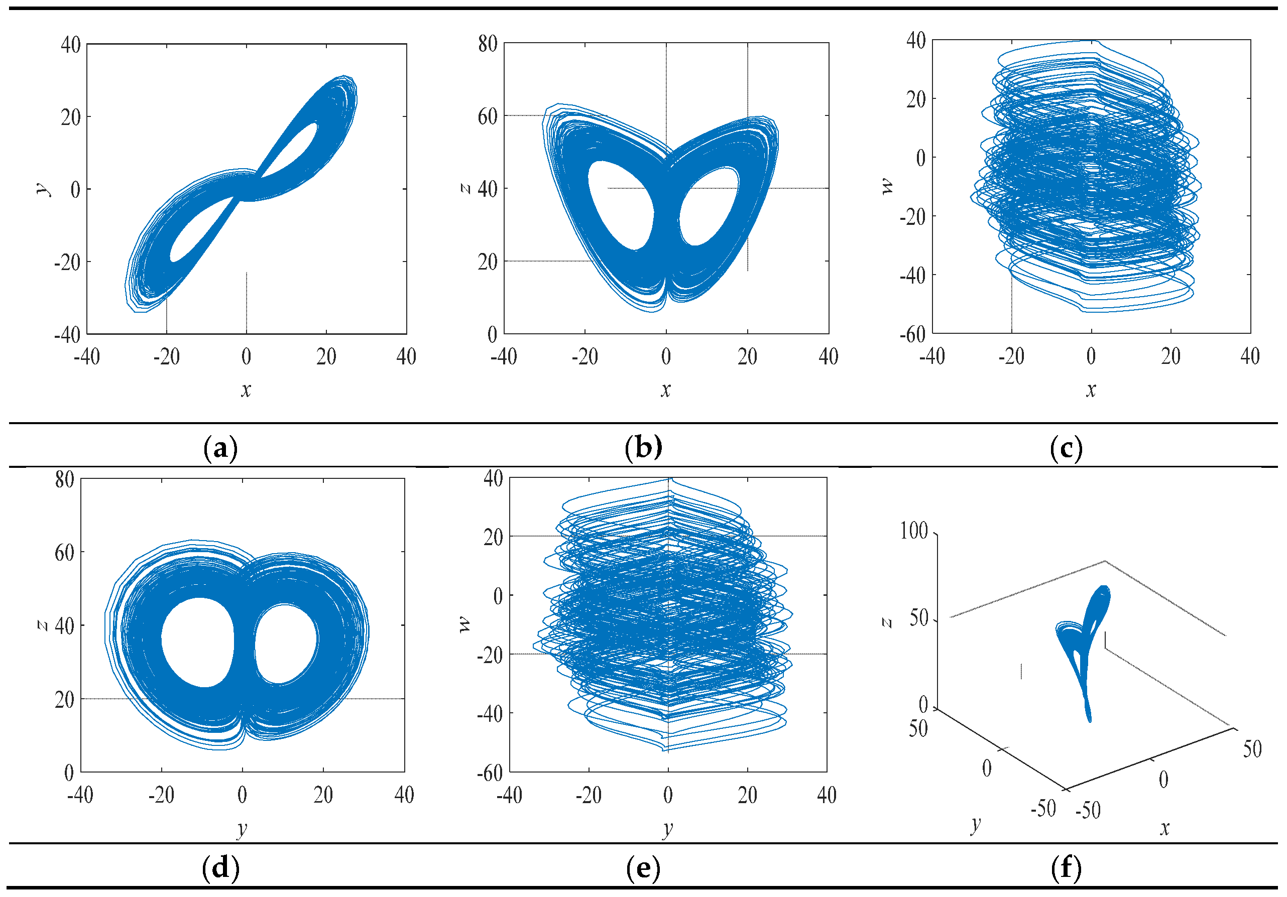
2.2. Hyperchaotic System

Since the hyperchaotic system contains more than two positive Lyapunov exponents, its chaotic properties are better, and its trajectory is more unpredictable. When a hyperchaotic system is applied to image encryption, the cryptosystem has a larger key space. The 4D hyperchaotic system utilized in this paper [29] is defined as follows:

$$\{\begin{array}{l}\dot{\mathrm{x}}=\mathsf{\lambda }(\mathrm{y}-\mathrm{x})+{\mathsf{\beta }}_1\mathrm{w}\\ \dot{\mathrm{y}}=\mathsf{\alpha }\mathrm{x}-\mathrm{x}\mathrm{z}+{\mathsf{\beta }}_2\mathrm{w}\\ \dot{\mathrm{z}}=-\mathsf{\sigma }\mathrm{z}+\mathrm{x}\mathrm{y}+{\mathsf{\beta }}_3\mathrm{w}\\ \dot{\mathrm{w}}=-\mathsf{\delta }\mathrm{x}\end{array},$$

(5)

where $\mathsf{\lambda }$, $\mathsf{\alpha }$, $\mathsf{\sigma }$, $\mathsf{\delta }$, ${\mathsf{\beta }}_1$, ${\mathsf{\beta }}_2$, and ${\mathsf{\beta }}_3$ are control parameters of the system. Only when $\mathsf{\lambda }=35$, $\mathsf{\alpha }=35$, $\mathsf{\sigma }=3$, $\mathsf{\delta }=5$, ${\mathsf{\beta }}_1=1$, ${\mathsf{\beta }}_2=0.2$, and ${\mathsf{\beta }}_3=0.3$, the system exhibits hyperchaotic behavior. Moreover, the phase trajectory of the system is displayed in Figure 3.

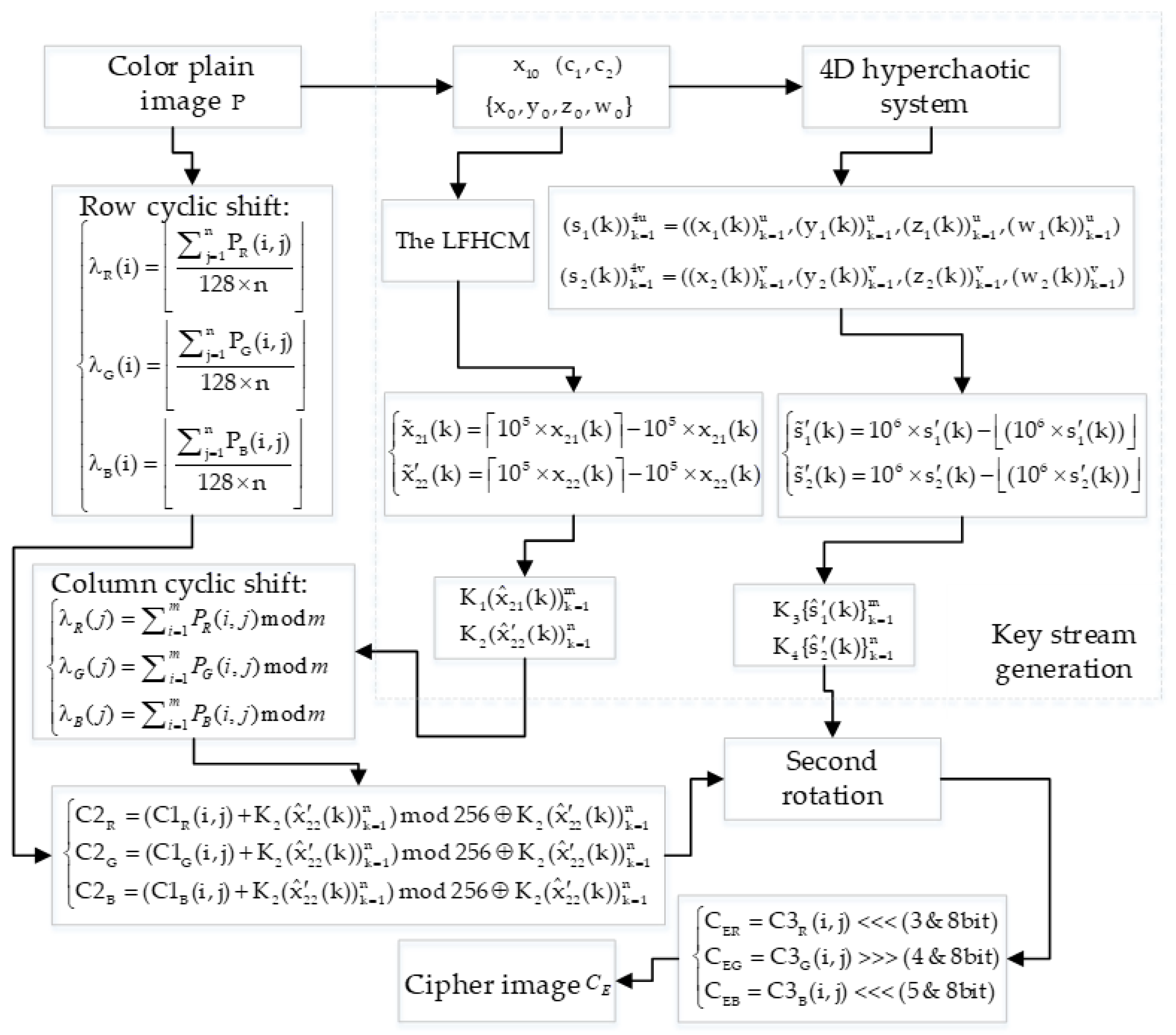
3. The Proposed Image Cryptosystem

3.1. Key Stream Generation

In this subsection, we introduce the key stream generation process of the encryption scheme in this paper. The specific steps are as follows:

Step 1: Decompose the plain image $\mathrm{P}$ of size $\mathrm{m}\times \mathrm{n}$ into three matrixes, ${\mathrm{P}}_{\mathrm{R}}$, ${\mathrm{P}}_{\mathrm{G}}$, and ${\mathrm{P}}_{\mathrm{B}}$. Set initial values ${\mathrm{x}}_{10}$ and $\{{\mathrm{x}}_0,{\mathrm{y}}_0,{\mathrm{z}}_0,{\mathrm{w}}_0\}$ for the LFHCM and 4D hyperchaotic system, respectively. Then apply the plain image $\mathrm{P}$ to update the initial values according to Equation (6)

$$\{\begin{array}{l}{\mathrm{x}}_{20}={\mathrm{x}}_{10}+\frac{{\displaystyle {\sum }_{\mathrm{i}=1}^{\mathrm{m}}{\displaystyle {\sum }_{\mathrm{j}=1}^{\mathrm{n}}{\mathrm{P}}_{\mathrm{R}}(\mathrm{i},\mathrm{j})}}}{{256}^3}\times \frac{{\mathrm{x}}_0+1}{{\mathrm{x}}_0+{\mathrm{y}}_0+{\mathrm{w}}_0+{\mathrm{z}}_0+2}\\ {\mathrm{x}}_{20}{}^{\prime }={\mathrm{x}}_{10}+\frac{{\displaystyle {\sum }_{\mathrm{i}=1}^{\mathrm{m}}{\displaystyle {\sum }_{\mathrm{j}=1}^{\mathrm{n}}{\mathrm{P}}_{\mathrm{R}}(\mathrm{i},\mathrm{j})}}}{2\times {256}^3}\times \frac{{\mathrm{y}}_0+{\mathrm{z}}_0+1}{{\mathrm{x}}_0+{\mathrm{y}}_0+{\mathrm{w}}_0+{\mathrm{z}}_0+2}\end{array}$$

(6)

$$\{\begin{array}{l}{{\mathrm{x}}^{\prime }}_0={\mathrm{x}}_0+\frac{{\displaystyle {\sum }_{\mathrm{i}=1}^{\mathrm{m}}{\displaystyle {\sum }_{\mathrm{j}=1}^{\mathrm{n}}{\mathrm{P}}_{\mathrm{G}}(\mathrm{i},\mathrm{j})}}}{{256}^2}\times \frac{{\mathrm{y}}_0+1}{{\mathrm{x}}_{10}+{\mathrm{y}}_0+{\mathrm{w}}_0+2}\\ {\mathrm{y}}_0{}^{\prime }={\mathrm{y}}_0+\frac{{\displaystyle {\sum }_{\mathrm{i}=1}^{\mathrm{m}}{\displaystyle {\sum }_{\mathrm{j}=1}^{\mathrm{n}}{\mathrm{P}}_{\mathrm{G}}(\mathrm{i},\mathrm{j})}}}{2\times {256}^2}\times \frac{{\mathrm{z}}_0+1}{{\mathrm{x}}_{10}+{\mathrm{x}}_0+{\mathrm{z}}_0+2}\\ {{\mathrm{z}}^{\prime }}_0={\mathrm{z}}_0+\frac{{\displaystyle {\sum }_{\mathrm{i}=1}^{\mathrm{m}-1}{\displaystyle {\sum }_{\mathrm{j}=1}^{\mathrm{n}}{\mathrm{P}}_{\mathrm{B}}(\mathrm{i},\mathrm{j})}}}{3\times {256}^3}\times \frac{{\mathrm{w}}_0+1}{{\mathrm{x}}_{10}+{\mathrm{y}}_0+{\mathrm{w}}_0+2}\\ {\mathrm{w}}_0{}^{\prime }={\mathrm{w}}_0+\frac{{\displaystyle {\sum }_{\mathrm{i}=1}^{\mathrm{m}}{\displaystyle {\sum }_{\mathrm{j}=1}^{\mathrm{n}-1}{\mathrm{P}}_{\mathrm{B}}(\mathrm{i},\mathrm{j})}}}{4\times {256}^3}\times \frac{{\mathrm{x}}_0+1}{{\mathrm{x}}_{10}+{\mathrm{x}}_0+{\mathrm{z}}_0+2}\end{array}$$

(7)

Step 2: Select two control parameters $\{{\mathrm{c}}_1,{\mathrm{c}}_2\}$ for the LFHCM, and iterate it $(\mathrm{m}+500)$ and $(\mathrm{n}+500)$ times with the initial values $\{{\mathrm{x}}_{20},{\mathrm{x}}_{20}{}^{\prime }\}$. Discard the first 500 elements to form two chaotic sequences, labeled ${({\mathrm{x}}_{21}(\mathrm{k}))}_{\mathrm{k}=1}^{\mathrm{m}}$ and ${({\mathrm{x}}_{22}(\mathrm{k}))}_{\mathrm{k}=1}^{\mathrm{n}}$.

Step 3: Pre-iterate the 4D hyperchaotic system described in the former section 1000 times. Then, iterate another $\mathrm{u}$ and $\mathrm{v}$ times to generate two pseudo-random sequences, ${\mathrm{s}}_1(\mathrm{k})$ and ${\mathrm{s}}_2(\mathrm{k})$, with initial values $\{{\mathrm{x}}_0{}^{\prime },{{\mathrm{y}}^{\prime }}_0,{{\mathrm{z}}^{\prime }}_0,{{\mathrm{w}}^{\prime }}_0\},$ respectively. They can be defined as follows:

$$\{\begin{array}{l}\mathrm{u}=\lceil (\mathrm{m}+1)/4\rceil \\ \mathrm{v}=\lceil (\mathrm{n}+1)/4\rceil \end{array}$$

(8)

$${({\mathrm{s}}_1(\mathrm{k}))}_{\mathrm{k}=1}^{4\mathrm{u}}=({({\mathrm{x}}_1(\mathrm{k}))}_{\mathrm{k}=1}^{\mathrm{u}},{({\mathrm{y}}_1(\mathrm{k}))}_{\mathrm{k}=1}^{\mathrm{u}},{({\mathrm{z}}_1(\mathrm{k}))}_{\mathrm{k}=1}^{\mathrm{u}},{({\mathrm{w}}_1(\mathrm{k}))}_{\mathrm{k}=1}^{\mathrm{u}})$$

(9)

$${({\mathrm{s}}_2(\mathrm{k}))}_{\mathrm{k}=1}^{4\mathrm{v}}=({({\mathrm{x}}_2(\mathrm{k}))}_{\mathrm{k}=1}^{\mathrm{v}},{({\mathrm{y}}_2(\mathrm{k}))}_{\mathrm{k}=1}^{\mathrm{v}},{({\mathrm{z}}_2(\mathrm{k}))}_{\mathrm{k}=1}^{\mathrm{v}},{({\mathrm{w}}_2(\mathrm{k}))}_{\mathrm{k}=1}^{\mathrm{v}})$$

(10)

where $\lceil ·\rceil$ denotes that the element returns the smallest integer in the infinite direction. Then, arbitrarily intercept $\mathrm{m}$ and $\mathrm{n}$ elements corresponding to the sequences ${({\mathrm{s}}_1(\mathrm{k}))}_{\mathrm{k}=1}^{4\mathrm{u}}$ and ${({\mathrm{s}}_2(\mathrm{k}))}_{\mathrm{k}=1}^{4\mathrm{v}}$ to produce sequences ${({\mathrm{s}}_1{}^{\prime }(\mathrm{k}))}_{\mathrm{k}=1}^{\mathrm{m}}$ and ${({\mathrm{s}}_2{}^{\prime }(\mathrm{k}))}_{\mathrm{k}=1}^{\mathrm{n}}$.

Step 4: Perform the following operations for the four chaotic sequences, ${({\mathrm{x}}_{21}(\mathrm{k}))}_{\mathrm{k}=1}^{\mathrm{m}},$ ${({\mathrm{x}}_{22}(\mathrm{k}))}_{\mathrm{k}=1}^{\mathrm{n}},$ ${({\mathrm{s}}_1{}^{\prime }(\mathrm{k}))}_{\mathrm{k}=1}^{\mathrm{m}},$ and ${({\mathrm{s}}_2{}^{\prime }(\mathrm{k}))}_{\mathrm{k}=1}^{\mathrm{n}}$ constructed in Step 2 and Step 3:

$$\{\begin{array}{l}{\tilde{\mathrm{x}}}_{21}(\mathrm{k})=\lceil {10}^5\times {\mathrm{x}}_{21}(\mathrm{k})\rceil -{10}^5\times {\mathrm{x}}_{21}(\mathrm{k})\\ {{\tilde{\mathrm{x}}}^{\prime }}_{22}(\mathrm{k})=\lceil {10}^5\times {\mathrm{x}}_{22}(\mathrm{k})\rceil -{10}^5\times {\mathrm{x}}_{22}(\mathrm{k})\end{array}$$

(11)

$$\{\begin{array}{l}{{\tilde{\mathrm{s}}}^{\prime }}_1(\mathrm{k})={10}^6\times {{\mathrm{s}}^{\prime }}_1(\mathrm{k})-\lfloor ({10}^6\times {{\mathrm{s}}^{\prime }}_1(\mathrm{k}))\rfloor \\ {{\tilde{\mathrm{s}}}^{\prime }}_2(\mathrm{k})={10}^6\times {{\mathrm{s}}^{\prime }}_2(\mathrm{k})-\lfloor ({10}^6\times {{\mathrm{s}}^{\prime }}_2(\mathrm{k}))\rfloor \end{array}$$

(12)

where $\lfloor ·\rfloor$ represents the function that make the element return the nearest integer towards minus infinity.

Step 5: Further convert these sequences according to Formulas (13) and (14).

$$\{\begin{array}{l}{\widehat{\mathrm{x}}}_{21}(\mathrm{k})=\lfloor {\tilde{\mathrm{x}}}_{21}(\mathrm{k})\times 1000\rfloor \mathrm{mod}\mathrm{m}+1\\ {{\widehat{\mathrm{x}}}^{\prime }}_{22}(\mathrm{k})=\lfloor {\tilde{\mathrm{x}}}_{22}(\mathrm{k})\times 1000\rfloor \mathrm{mod}\mathrm{n}+1\end{array}$$

(13)

$$\{\begin{array}{l}{{\widehat{\mathrm{s}}}^{\prime }}_1(\mathrm{k})=\mathrm{f}\mathrm{i}\mathrm{x}((({\widetilde{{\mathrm{s}}^{\prime }}}_1(\mathrm{k})+100)\mathrm{mod}1)\times {10}^{12}\mathrm{mod}\mathrm{m})+1\\ {{\widehat{\mathrm{s}}}^{\prime }}_2(\mathrm{k})=\mathrm{f}\mathrm{i}\mathrm{x}((({\widetilde{{\mathrm{s}}^{\prime }}}_2(\mathrm{k})+500)\mathrm{mod}1)\times {10}^{12}\mathrm{mod}\mathrm{n})+1\end{array},$$

(14)

The resulting four sequences are treated as key streams that can be expressed as ${\mathrm{K}}_1{({\widehat{\mathrm{x}}}_{21}(\mathrm{k}))}_{\mathrm{k}=1}^{\mathrm{m}}$, ${\mathrm{K}}_2{({{\widehat{\mathrm{x}}}^{\prime }}_{22}(\mathrm{k}))}_{\mathrm{k}=1}^{\mathrm{n}}$, ${\mathrm{K}}_3{\{{{\widehat{\mathrm{s}}}^{\prime }}_1(\mathrm{k})\}}_{\mathrm{k}=1}^{\mathrm{m}}$ and ${\mathrm{K}}_4{\{{{\widehat{\mathrm{s}}}^{\prime }}_2(\mathrm{k})\}}_{\mathrm{k}=1}^{\mathrm{n}}$.

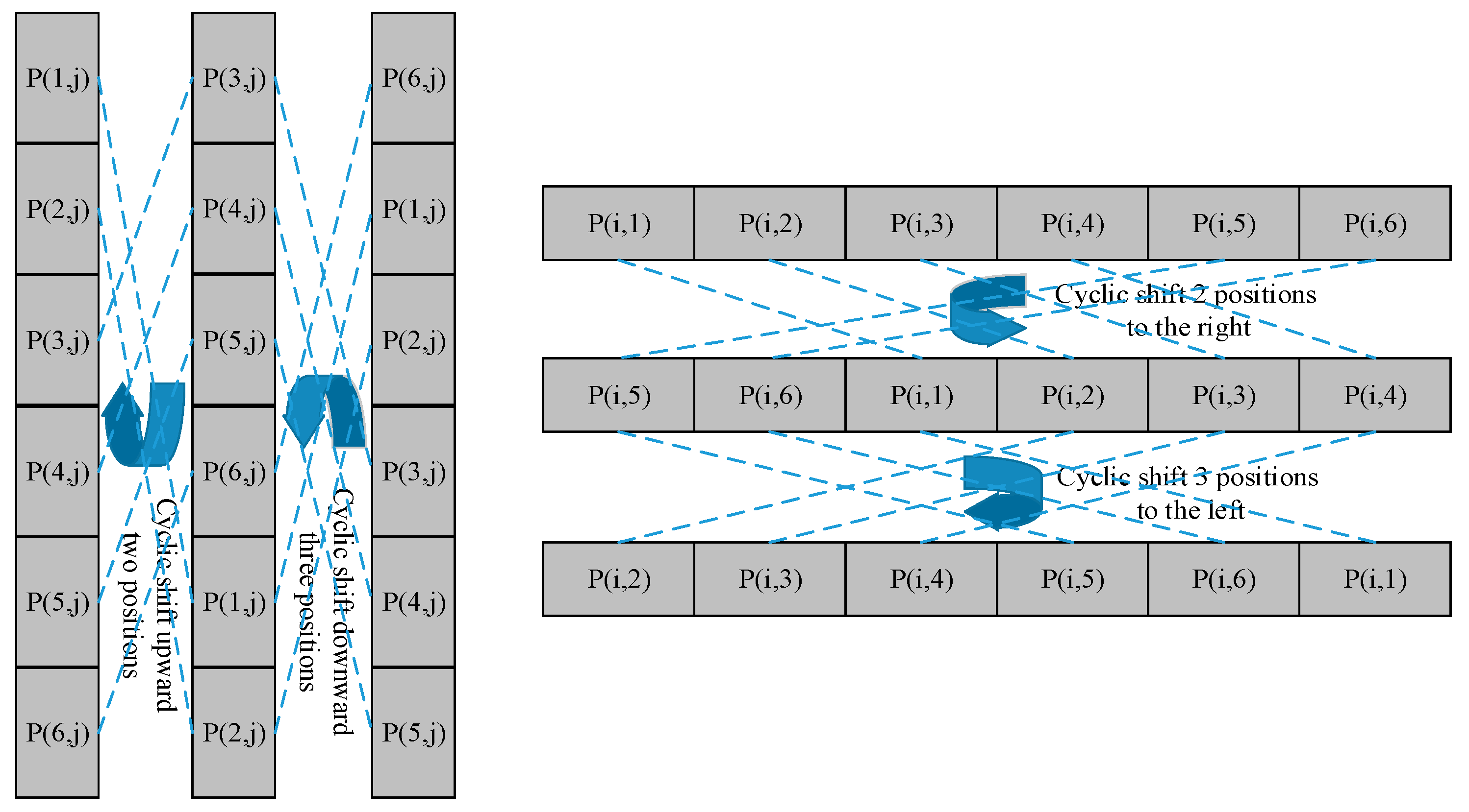
3.2. Encryption Scheme

Input: Color plain image $\mathrm{P}$ of size $\mathrm{m}\times \mathrm{n}.$ Output: Color cipher image of the same size.

Step 1: Calculate the initial conditions based on the plain image $\mathrm{P}$, and set the control parameters $\{{\mathrm{c}}_1,{\mathrm{c}}_2\}$ for the LFHCM. After selecting the initial values for the 4D hyperchaotic system, the key streams ${\mathrm{K}}_1{({\widehat{\mathrm{x}}}_{21}(\mathrm{k}))}_{\mathrm{k}=1}^{\mathrm{m}}$, ${\mathrm{K}}_2{({{\widehat{\mathrm{x}}}^{\prime }}_{22}(\mathrm{k}))}_{\mathrm{k}=1}^{\mathrm{n}}$, ${\mathrm{K}}_3{\{{{\widehat{\mathrm{s}}}^{\prime }}_1(\mathrm{k})\}}_{\mathrm{k}=1}^{\mathrm{m}}$ and ${\mathrm{K}}_4{\{{{\widehat{\mathrm{s}}}^{\prime }}_1(\mathrm{k})\}}_{\mathrm{k}=1}^{\mathrm{m}}$ are generated by the preceding subsection.

Step 2: The color plain image is decomposed into three matrixes of ${\mathrm{P}}_{\mathrm{R}}$, ${\mathrm{P}}_{\mathrm{G}}$, and ${\mathrm{P}}_{\mathrm{B}}$, then each row $\mathrm{i}$ of the three matrixes is subjected to Equation (15).

$$\{\begin{array}{l}{\mathsf{\lambda }}_{\mathrm{R}}(\mathrm{i})=\lfloor \frac{{\displaystyle {\sum }_{\mathrm{j}=1}^{\mathrm{n}}{\mathrm{P}}_{\mathrm{R}}(\mathrm{i},\mathrm{j})}}{128\times \mathrm{n}}\rfloor \\ {\mathsf{\lambda }}_{\mathrm{G}}(\mathrm{i})=\lfloor \frac{{\displaystyle {\sum }_{\mathrm{j}=1}^{\mathrm{n}}{\mathrm{P}}_{\mathrm{G}}(\mathrm{i},\mathrm{j})}}{128\times \mathrm{n}}\rfloor \\ {\mathsf{\lambda }}_{\mathrm{B}}(\mathrm{i})=\lfloor \frac{{\displaystyle {\sum }_{\mathrm{j}=1}^{\mathrm{n}}{\mathrm{P}}_{\mathrm{B}}(\mathrm{i},\mathrm{j})}}{128\times \mathrm{n}}\rfloor \end{array}$$

(15)

When the computed values ${\mathsf{\lambda }}_{\mathrm{R},\mathrm{G},\mathrm{B}}(\mathrm{i})=0$, the ${\mathrm{P}}_{\mathrm{R}}$, ${\mathrm{P}}_{\mathrm{G}}$, and ${\mathrm{P}}_{\mathrm{B}}$ matrixes are respectively cyclically shifted to the left by ${\mathrm{K}}_1{({\widehat{\mathrm{x}}}_{21}(\mathrm{k}))}_{\mathrm{k}=1}^{\mathrm{m}}$ positions, where $\mathrm{k}=\mathrm{i}.$ Then, when ${\mathsf{\lambda }}_{\mathrm{R},\mathrm{G},\mathrm{B}}(\mathrm{i})=1$, the cyclic shifts are performed correspondingly to the right ${\mathrm{K}}_1{\{{\widehat{\mathrm{x}}}_{21}(\mathrm{k})\}}_{\mathrm{k}=1}^{\mathrm{m}}$ positions. As shown in Figure 4, similar to the principle of Rubik’s Cube, the pixels of the image can also be rotated and shifted to the left and right.

Step 3: For each column of ${\mathrm{P}}_{\mathrm{R}}$, ${\mathrm{P}}_{\mathrm{G}}$, and ${\mathrm{P}}_{\mathrm{B}}$, the operations are as follows:

$$\{\begin{array}{l}{\mathsf{\lambda }}_{\mathrm{R}}(\mathrm{j})={\displaystyle {\sum }_{\mathrm{i}=1}^{\mathrm{m}}{\mathrm{P}}_{\mathrm{R}}(\mathrm{i},\mathrm{j})}\mathrm{mod}\mathrm{m}\\ {\mathsf{\lambda }}_{\mathrm{G}}(\mathrm{j})={\displaystyle {\sum }_{\mathrm{i}=1}^{\mathrm{m}}{\mathrm{P}}_{\mathrm{G}}(\mathrm{i},\mathrm{j})}\mathrm{mod}\mathrm{m}\\ {\mathsf{\lambda }}_{\mathrm{B}}(\mathrm{j})={\displaystyle {\sum }_{\mathrm{i}=1}^{\mathrm{m}}{\mathrm{P}}_{\mathrm{B}}(\mathrm{i},\mathrm{j})}\mathrm{mod}\mathrm{m}\end{array}$$

(16)

When the calculated values ${\mathsf{\lambda }}_{\mathrm{R},\mathrm{G},\mathrm{B}}(\mathrm{j})>128$, the ${\mathrm{P}}_{\mathrm{R}}$, ${\mathrm{P}}_{\mathrm{G}}$, and ${\mathrm{P}}_{\mathrm{B}}$ matrixes are respectively cyclically shifted upward by ${\mathrm{K}}_2{({{\widehat{\mathrm{x}}}^{\prime }}_{22}(\mathrm{k}))}_{\mathrm{k}=1}^{\mathrm{n}}$ positions, where $\mathrm{k}=\mathrm{j}$. Then, when ${\mathsf{\lambda }}_{\mathrm{R},\mathrm{G},\mathrm{B}}(\mathrm{j})\le 128$, the cyclic shifts are performed correspondingly downward to ${\mathrm{K}}_2{({{\widehat{\mathrm{x}}}^{\prime }}_{22}(\mathrm{k}))}_{\mathrm{k}=1}^{\mathrm{n}}$ positions. The upward and downward cyclic shift diagram is also displayed in Figure 4, and three scrambled matrixes, $\mathrm{C}{1}_{\mathrm{R}},$ $\mathrm{C}{1}_{\mathrm{G}},$ and $\mathrm{C}{1}_{\mathrm{B}}$, are obtained.

Step 4: Execute bit-wise diffusion operation on each row of the matrixes $\mathrm{C}{1}_{\mathrm{R}}$, $\mathrm{C}{1}_{\mathrm{G}}$, and $\mathrm{C}{1}_{\mathrm{B}}$ according to Equation (17).

$$\{\begin{array}{l}\mathrm{C}{2}_{\mathrm{R}}=(\mathrm{C}{1}_{\mathrm{R}}(\mathrm{i},\mathrm{j})+{\mathrm{K}}_2{({{\widehat{\mathrm{x}}}^{\prime }}_{22}(\mathrm{k}))}_{\mathrm{k}=1}^{\mathrm{n}})\mathrm{mod}256\oplus {\mathrm{K}}_2{({{\widehat{\mathrm{x}}}^{\prime }}_{22}(\mathrm{k}))}_{\mathrm{k}=1}^{\mathrm{n}}\\ \mathrm{C}{2}_{\mathrm{G}}=(\mathrm{C}{1}_{\mathrm{G}}(\mathrm{i},\mathrm{j})+{\mathrm{K}}_2{({{\widehat{\mathrm{x}}}^{\prime }}_{22}(\mathrm{k}))}_{\mathrm{k}=1}^{\mathrm{n}})\mathrm{mod}256\oplus {\mathrm{K}}_2{({{\widehat{\mathrm{x}}}^{\prime }}_{22}(\mathrm{k}))}_{\mathrm{k}=1}^{\mathrm{n}}\\ \mathrm{C}{2}_{\mathrm{B}}=(\mathrm{C}{1}_{\mathrm{B}}(\mathrm{i},\mathrm{j})+{\mathrm{K}}_2{({{\widehat{\mathrm{x}}}^{\prime }}_{22}(\mathrm{k}))}_{\mathrm{k}=1}^{\mathrm{n}})\mathrm{mod}256\oplus {\mathrm{K}}_2{({{\widehat{\mathrm{x}}}^{\prime }}_{22}(\mathrm{k}))}_{\mathrm{k}=1}^{\mathrm{n}}\end{array}$$

(17)

Step 5: For the odd rows of the matrixes $\mathrm{C}{2}_{\mathrm{R}}$, $\mathrm{C}{2}_{\mathrm{G}}$, and $\mathrm{C}{2}_{\mathrm{B}}$, they are cyclically shifted to the left by ${\mathrm{K}}_3{\{{{\widehat{\mathrm{s}}}^{\prime }}_1(\mathrm{k})\}}_{\mathrm{k}=1}^{\mathrm{m}}$ positions, and the even rows are rotated to the right by the same positions. Meanwhile, for the odd columns of the matrixes $\mathrm{C}{2}_{\mathrm{R}}$, $\mathrm{C}{2}_{\mathrm{G}}$, and $\mathrm{C}{2}_{\mathrm{B}}$, they are respectively cycle shifted upward by ${\mathrm{K}}_4{\{{{\widehat{\mathrm{s}}}^{\prime }}_2(\mathrm{k})\}}_{\mathrm{k}=1}^{\mathrm{n}}$ positions, and the even columns are correspondingly shifted downward by the same positions. Then, three disordered matrixes, $\mathrm{C}{3}_{\mathrm{R}}$, $\mathrm{C}{3}_{\mathrm{G}}$, and $\mathrm{C}{3}_{\mathrm{B}}$, are produced.

Step 6: Finally, a bit-level scrambling is implemented by the following formula:

$$\{\begin{array}{l}{\mathrm{C}}_{\mathrm{E}\mathrm{R}}=\mathrm{C}{3}_{\mathrm{R}}(\mathrm{i},\mathrm{j})<<<(3\&8\mathrm{b}\mathrm{i}\mathrm{t})\\ {\mathrm{C}}_{\mathrm{E}\mathrm{G}}=\mathrm{C}{3}_{\mathrm{G}}(\mathrm{i},\mathrm{j})>>>(4\&8\mathrm{b}\mathrm{i}\mathrm{t})\\ {\mathrm{C}}_{\mathrm{E}\mathrm{B}}=\mathrm{C}{3}_{\mathrm{B}}(\mathrm{i},\mathrm{j})<<<(5\&8\mathrm{b}\mathrm{i}\mathrm{t})\end{array}$$

(18)

Merge the three components, ${\mathrm{C}}_{\mathrm{E}\mathrm{R}}$, ${\mathrm{C}}_{\mathrm{E}\mathrm{G}}$, and ${\mathrm{C}}_{\mathrm{E}\mathrm{B}}$, to form the final encrypted image ${\mathrm{C}}_{\mathrm{E}}$. The flowchart of our encryption scheme is displayed in Figure 5.

3.3. Decryption Scheme

The decryption procedure is the inverse process of the encryption scheme, and it can be described briefly as follows:

Step 1: Apply the same initial conditions as encryption to iterate Equations (1) and (9) to generate the key streams ${\mathrm{K}}_1{({\widehat{\mathrm{x}}}_{21}(\mathrm{k}))}_{\mathrm{k}=1}^{\mathrm{m}}$, ${\mathrm{K}}_2{({{\widehat{\mathrm{x}}}^{\prime }}_{22}(\mathrm{k}))}_{\mathrm{k}=1}^{\mathrm{n}}$, ${\mathrm{K}}_3{\{{{\widehat{\mathrm{s}}}^{\prime }}_1(\mathrm{k})\}}_{\mathrm{k}=1}^{\mathrm{m}}$ and ${\mathrm{K}}_4{\{{{\widehat{\mathrm{s}}}^{\prime }}_2(\mathrm{k})\}}_{\mathrm{k}=1}^{\mathrm{n}}$.

Step 2: Execute bit shift to the left or right of the components ${\mathrm{C}}_{\mathrm{E}\mathrm{R}}$, ${\mathrm{C}}_{\mathrm{E}\mathrm{G}}$, and ${\mathrm{C}}_{\mathrm{E}\mathrm{B}}$ to get the matrixes $\mathrm{C}{3}_{\mathrm{R}}$, $\mathrm{C}{3}_{\mathrm{G}}$, and $\mathrm{C}{3}_{\mathrm{B}}$.

Step 3: Cyclic shift the rows and columns of the matrixes $\mathrm{C}{3}_{\mathrm{R}}$, $\mathrm{C}{3}_{\mathrm{G}}$, and $\mathrm{C}{3}_{\mathrm{B}}$ according to the opposite direction of step 5 in the previous subsection, then the matrixes $\mathrm{C}{2}_{\mathrm{R}}$, $\mathrm{C}{2}_{\mathrm{G}}$, and $\mathrm{C}{2}_{\mathrm{B}}$ are acquired.

Step 4: Perform bit-wise operations utilizing Formula (19).

$$\{\begin{array}{l}\mathrm{C}{1}_{\mathrm{R}}=(\mathrm{C}{2}_{\mathrm{R}}(\mathrm{i},\mathrm{j})\oplus {\mathrm{K}}_2{({{\widehat{\mathrm{x}}}^{\prime }}_{22}(\mathrm{k}))}_{\mathrm{k}=1}^{\mathrm{n}}+256-{\mathrm{K}}_2{({{\widehat{\mathrm{x}}}^{\prime }}_{22}(\mathrm{k}))}_{\mathrm{k}=1}^{\mathrm{n}})\mathrm{mod}256\\ \mathrm{C}{1}_{\mathrm{G}}=(\mathrm{C}{2}_{\mathrm{G}}(\mathrm{i},\mathrm{j})\oplus {\mathrm{K}}_2{({{\widehat{\mathrm{x}}}^{\prime }}_{22}(\mathrm{k}))}_{\mathrm{k}=1}^{\mathrm{n}}+256-{\mathrm{K}}_2{({{\widehat{\mathrm{x}}}^{\prime }}_{22}(\mathrm{k}))}_{\mathrm{k}=1}^{\mathrm{n}})\mathrm{mod}256\\ \mathrm{C}{1}_{\mathrm{B}}=(\mathrm{C}{2}_{\mathrm{B}}(\mathrm{i},\mathrm{j})\oplus {\mathrm{K}}_2{({{\widehat{\mathrm{x}}}^{\prime }}_{22}(\mathrm{k}))}_{\mathrm{k}=1}^{\mathrm{n}}+256-{\mathrm{K}}_2{({{\widehat{\mathrm{x}}}^{\prime }}_{22}(\mathrm{k}))}_{\mathrm{k}=1}^{\mathrm{n}})\mathrm{mod}256\end{array}$$

(19)

Step 5: Implement second reverse circular shifts on the rows and columns of the three matrices, $\mathrm{C}{1}_{\mathrm{R}}$, $\mathrm{C}{1}_{\mathrm{G}}$ and $\mathrm{C}{1}_{\mathrm{B}}$, according to Equations (15) and (16).

Step 6: Merge the three obtained matrixes to form the original image $\mathrm{P}$.

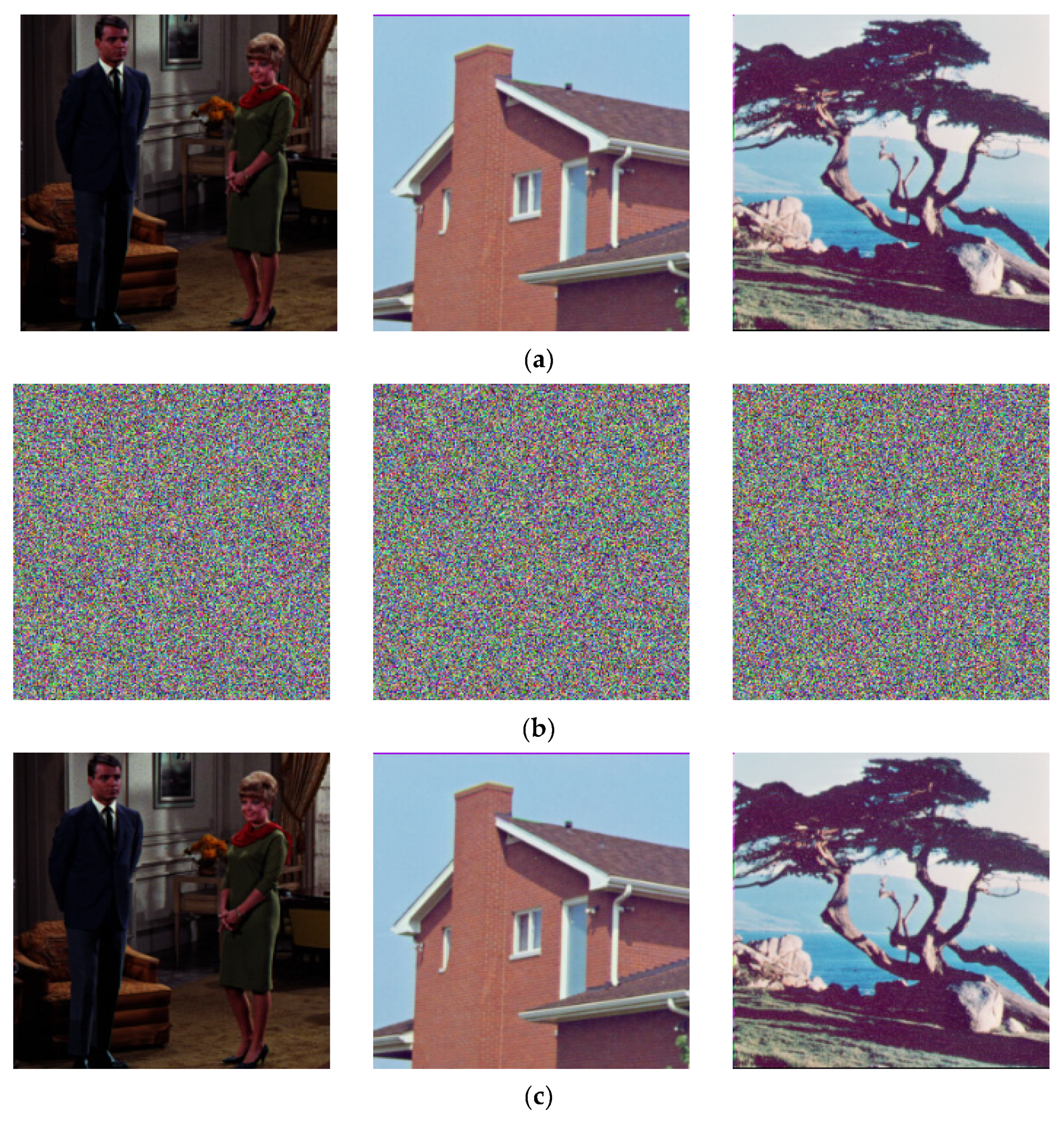
4. Experimental Results

As exhibited in Figure 6, three $256\times 256$ color plain images, “Couple”, “House” and “Tree”, were encrypted by python version 3.6 on a PC with an Intel Core i5, 3.4 GHz CPU, 8 GB memory. The noise-like phenomena appear in cipher images, which proves the feasibility of the scheme from the visual perspective

The encryption results are based on the following conditions:

${\mathrm{x}}_{10}=0.26534695122143,$${\mathrm{c}}_1=11.422,$${\mathrm{c}}_2=11.439,$${\mathrm{x}}_0=3.68526527215001,$${\mathrm{y}}_0=1.15265332455324,$${\mathrm{z}}_0=4.65289567518252,$${\mathrm{w}}_0=2.68526527217589.$

5. Performance Analysis

This section describes the performance analysis of our encryption scheme in terms of key space, key sensitivity, histogram analysis, correlation distribution, and information entropy evaluation, and so on.

5.1. Key Space

The key space is a collection of all legitimate keys. Only when it is large enough can it resist a variety of powerful attacks. Here the data range of the LFHCM is $[0,1.56]$, and the approximate intervals about the initial values of the 4D hyperchaotic system are ${\mathrm{x}}_0\in [-30,27]$, ${\mathrm{y}}_0\in [-34,30]$, ${\mathrm{z}}_0\in [6,63]$, and ${\mathrm{w}}_0\in [-52,40]$. In general, the precision of initial values and control numbers can reach ${10}^{-14}$. Thus, the size of the key space is able to achieve ${({10}^{14})}^7\times {10}^3={10}^{101}\approx 2^{335}\gg 2^{212}$ [24].

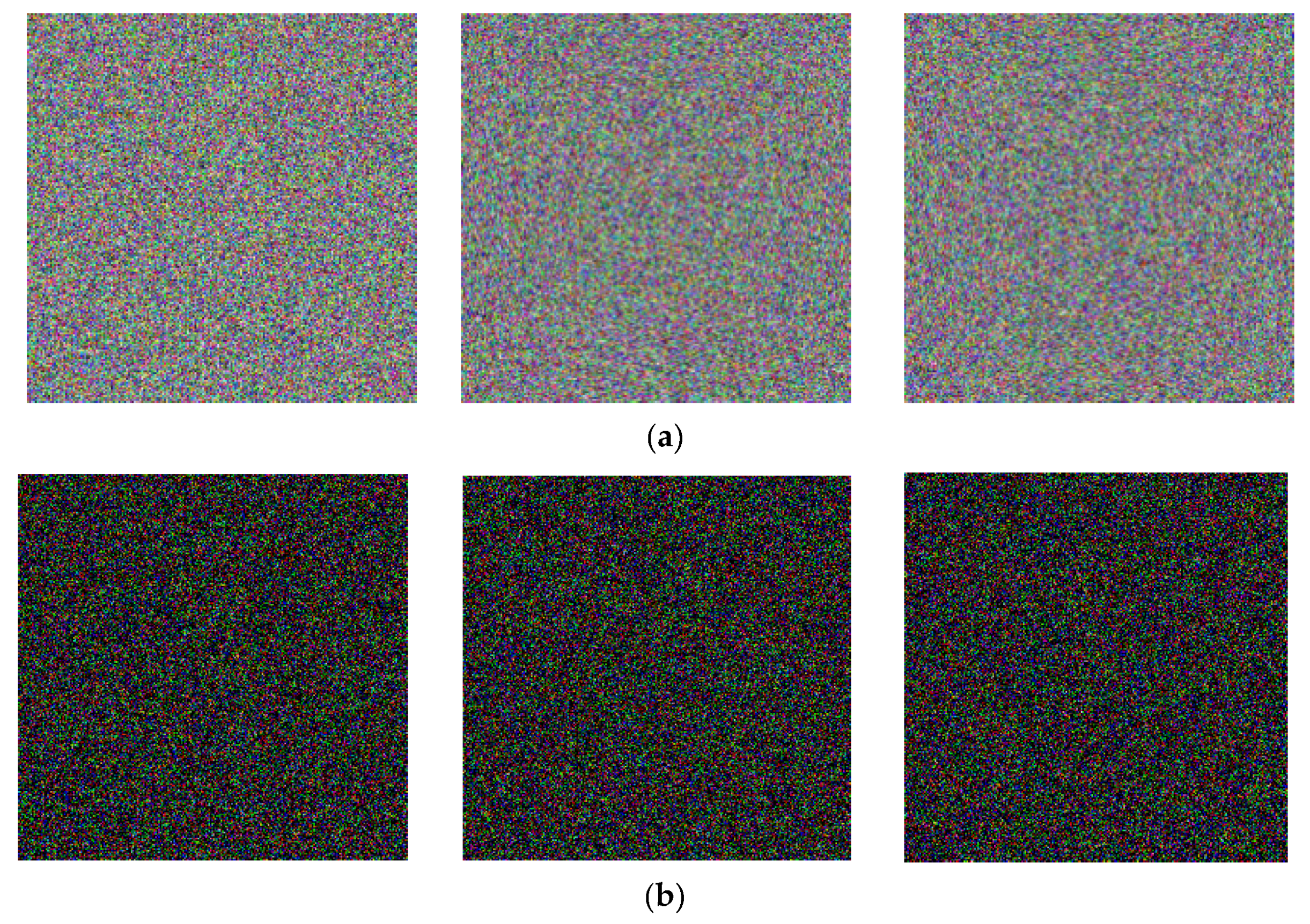
5.2. Key Sensitivity Analysis

The key sensitivity analysis is designed to observe the impact of small changes in the keys on cipher images. As for a chaotic map, the nuances of the initial conditions can produce two completely different sequences. Thus, we just changed initial value ${\mathrm{x}}_{10}$ with ${10}^{-14}$, then we re-encrypted the original images in Figure 6a. The cipher images in Figure 7a were obtained. Figure 7b exhibits the pixel-by-pixel difference between Figure 6b and Figure 7a, and it can be discovered that a subtle change to the keys can result in a completely different encryption. Moreover,

Table 4. Difference between cipher images with modified keys.

Modified Key	Difference Rate (%)
	Couple	House	Tree
${\mathrm{x}}_{10}+{10}^{-14}$	99.6155	99.5880	99.5931
${\mathrm{c}}_1+{10}^{-14}$	99.6094	99.6190	99.6089
${\mathrm{c}}_2+{10}^{-14}$	99.6043	99.6002	99.6007
${\mathrm{x}}_0+{10}^{-14}$	99.6190	99.6237	99.6038
${\mathrm{y}}_0+{10}^{-14}$	99.6038	99.6165	99.6185
${\mathrm{z}}_0+{10}^{-14}$	99.5956	99.6185	99.6048
${\mathrm{w}}_0+{10}^{-14}$	99.6140	99.5946	99.6063

lists the difference rates between two encrypted images with only one of the keys changed, and these data are greater than 99.5%. Therefore, we can conclude that our encryption scheme has strong key sensitivity.

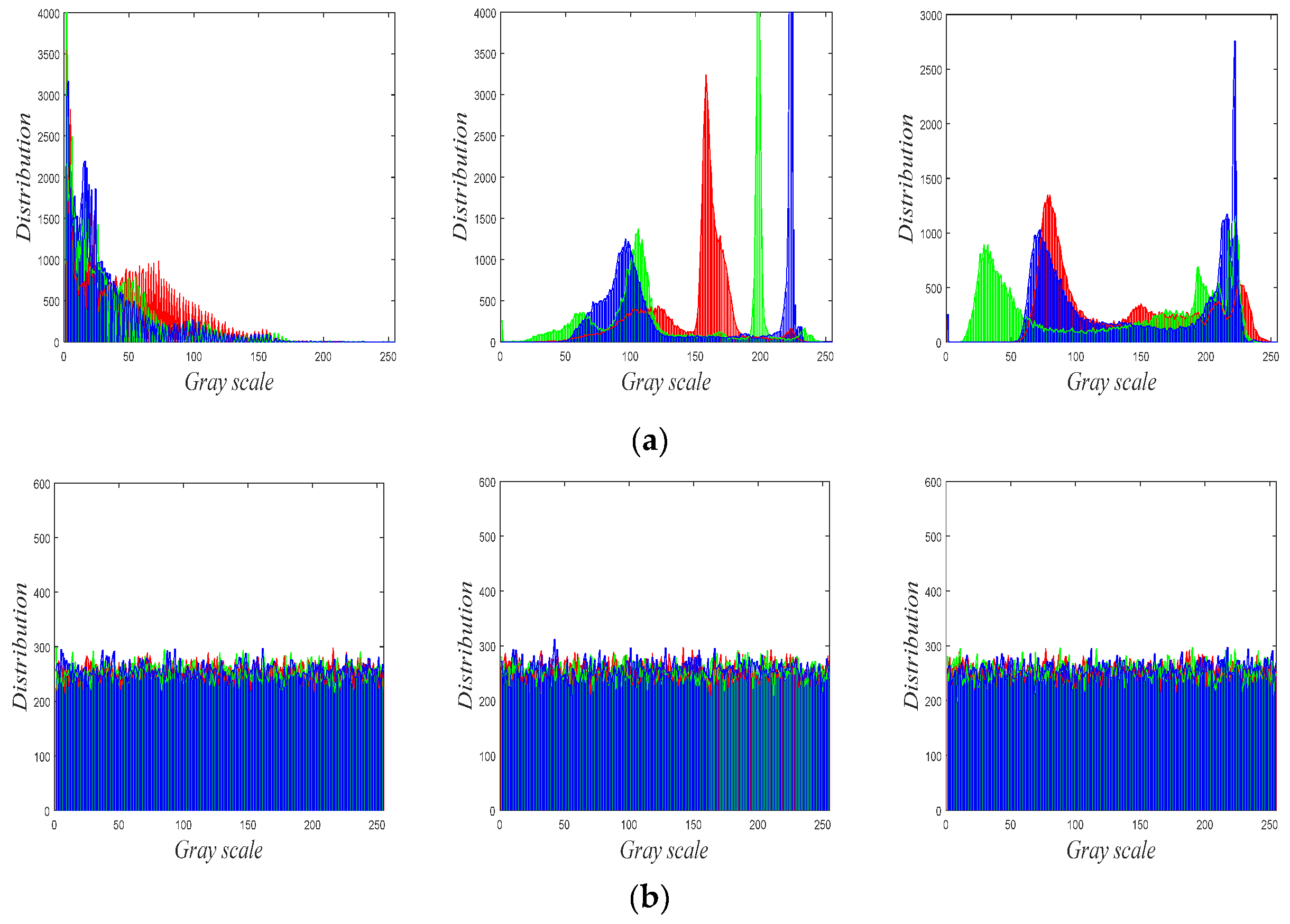
5.3. Histogram Analysis

The histogram is an important statistical feature of the image. An outstanding cryptosystem has the capacity to evenly distribute the histogram of the cipher image. In this case, the attacker cannot extract statistical features of the plain image from its cipher. Figure 8 presents the histograms of the plain and cipher images in Figure 7, which demonstrates that encryption makes the histogram information safely obscured.

In order to further verify the encryption effect, we used the statistical magnitude ${\mathsf{\chi }}^2$ to measure the pixel values distribution of the plain and cipher images, which can be defined as follows:

$${\mathsf{\chi }}^2={\displaystyle \sum _{\mathrm{i}=0}^{255}\frac{{({\mathrm{f}}_{\mathrm{i}}-{\mathrm{g}}_{\mathrm{i}})}^2}{{\mathrm{g}}_{\mathrm{i}}}}$$

(20)

where ${\mathrm{f}}_{\mathrm{i}}$ denotes occurrence frequency of pixel value $\mathrm{i}$, and ${\mathrm{g}}_{\mathrm{i}}$ represents the theoretical frequency of pixel value $\mathrm{i}$. As displayed in

Table 5. Chi-square test of plain and cipher images.

${\mathsf{\chi }}^2$	Plain Image			Cipher Image
	R	G	B	R	G	B
Couple	2.1036 × 105	3.3786 × 105	2.8964 × 105	247.6016	234.6563	249.8984
House	2.5858 × 105	2.9916 × 105	3.9404 × 105	274.3672	277.3203	286.9922
Tree	8.1371 × 104	5.7009 × 104	1.2982 × 104	254.0859	244.8125	264.3594
Lena	2.4628 × 105	1.1766 × 105	3.4033 × 105	257.1094	261.9063	202.1699
Peppers	5.4984 × 104	7.2077 × 104	1.1435 × 105	279.4395	268.0254	273.2910
Airplane	1.6115 × 105	1.5940 × 105	2.6505 × 105	234.2305	283.9785	243.3086
Lena in [30]	-	-	-	231.6144	248.36505	254.4806
Pepper in [30]	-	-	-	266.1728	273.2120	252.6552
Airplane in [30]	-	-	-	275.2378	271.7001	228.2813

, the chi-square test was performed on six images at a significant level of 0.05. Since the values are not only much smaller than the chi-square values of the plain images, but they are also lower than the critical value ${\mathsf{\chi }}_{0.05}^2(255)=293.24783$, they all pass the test. That is, our cryptosystem can effectively resist statistical attack.

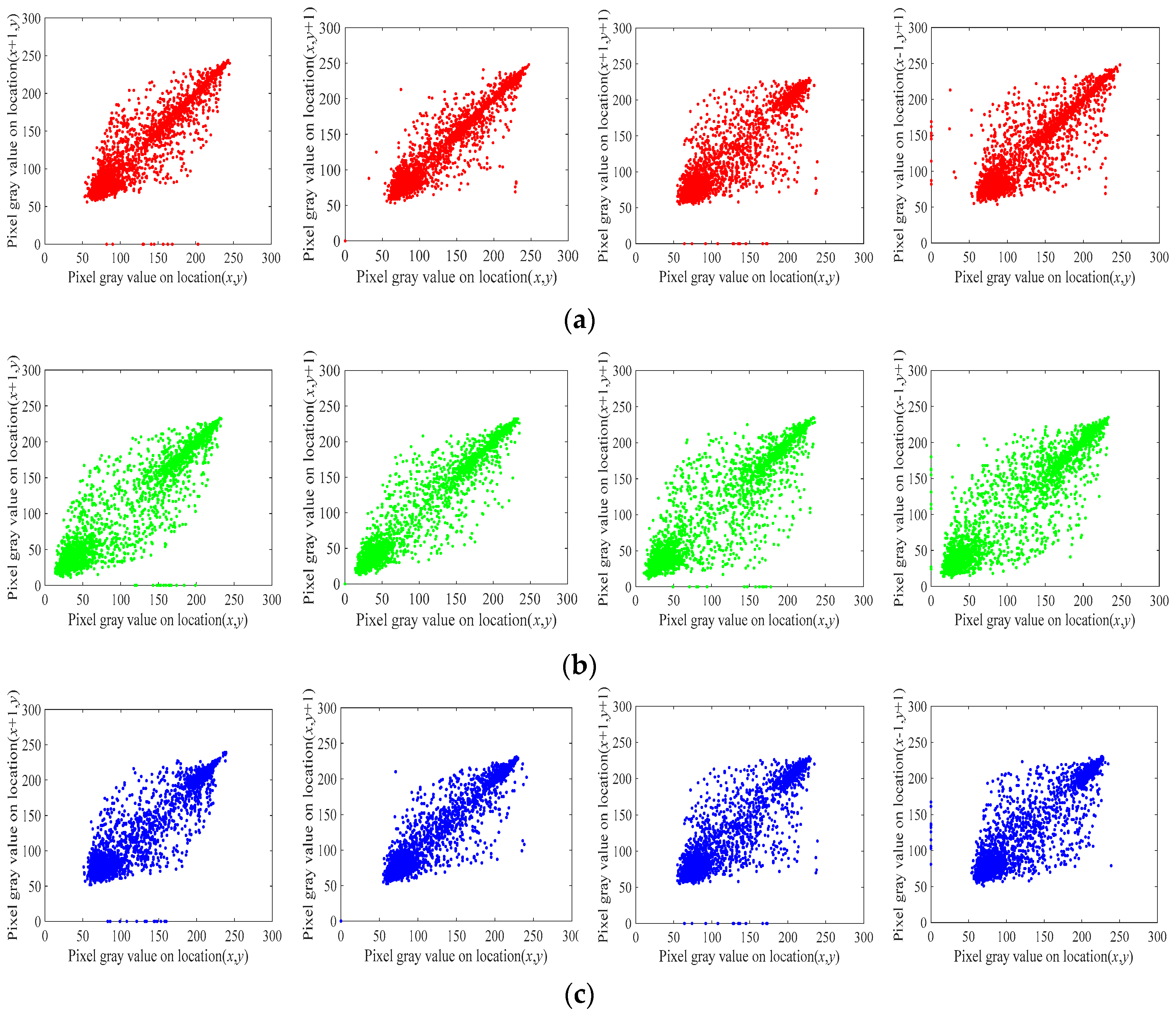
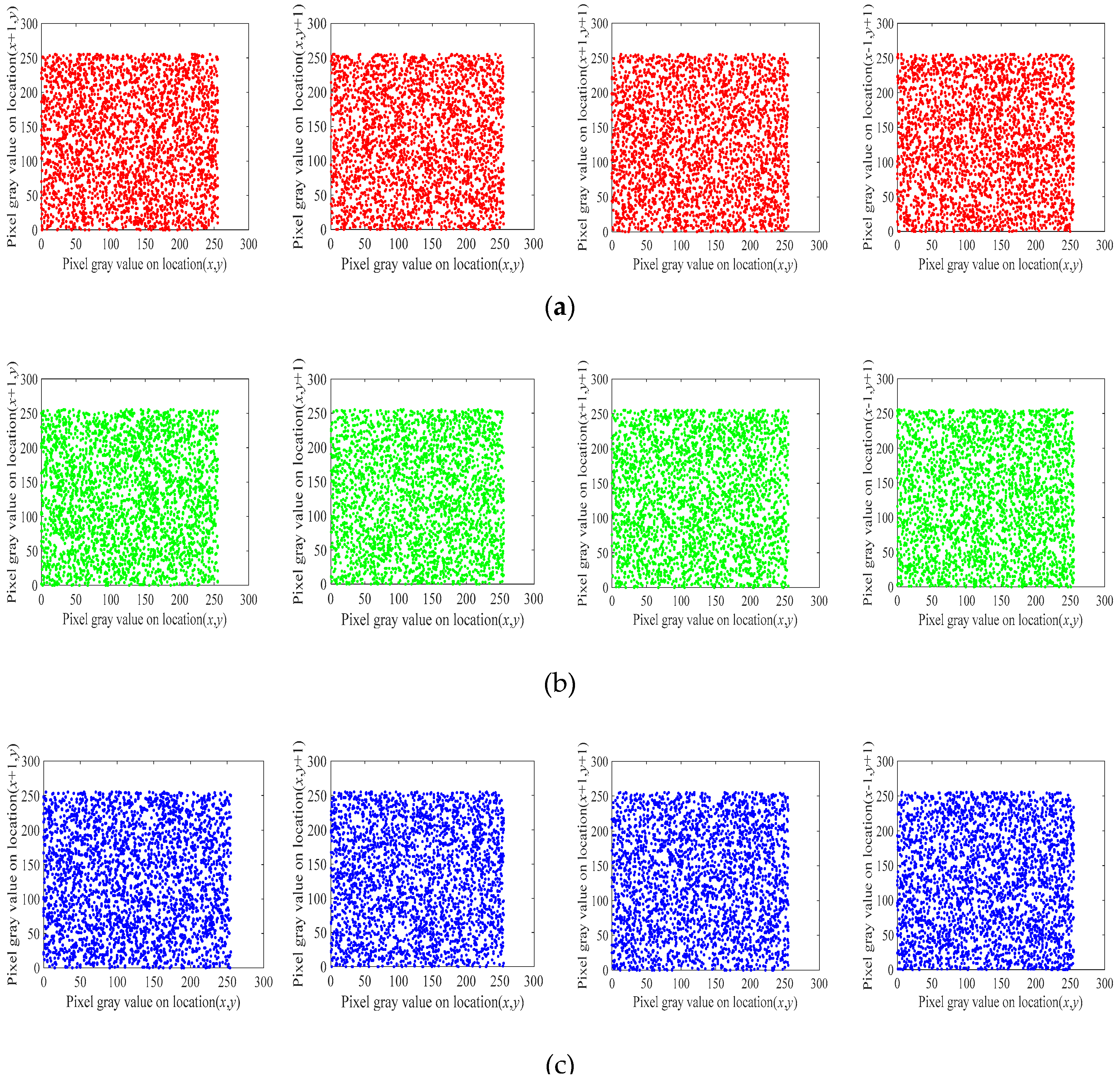
5.4. Correlation Analysis

The correlation of two adjacent pixels can reflect the degree of diffusion about image pixels. Figure 9 and Figure 10 exhibit the correlation distribution of the three channels, R, G and B, in the horizontal, vertical, main-diagonal and back-diagonal directions of the plain Tree image and cipher Tree image, respectively. Furthermore, we randomly chose 3000 pairs of adjacent pixels from a few original images and corresponding encrypted images. Then, we analyzed the correlation coefficients in horizontal, vertical, and main-diagonal directions according to Equation (21).

$${\mathsf{\rho }}_{\mathrm{x}\mathrm{y}}=\frac{\mathrm{E}[(\mathrm{x}-{\mathsf{\mu }}_{\mathrm{x}})(\mathrm{y}-{\mathsf{\mu }}_{\mathrm{y}})]}{{\mathsf{\sigma }}_{\mathrm{x}}{\mathsf{\sigma }}_{\mathrm{y}}}$$

(21)

where $\mathsf{\mu }$ and $\mathsf{\sigma }$ indicate the mean value and standard deviation. The results are shown in

Table 6. Correlation coefficients of plain images.

Image	Plain Image
	Horizontal	Vertical	Main-Diagonal	Back-Diagonal
Couple	0.9566	0.9566	0.9566	0.9566
House	0.9348	0.9693	0.9163	0.9588
Tree	0.9298	0.9542	0.9071	0.9047
Lena	0.9872	0.9756	0.9633	0.9709
Peppers	0.9466	0.9452	0.9100	0.9186
Baboon	0.8847	0.9099	0.8251	0.8120

and

Table 7. Correlation coefficients of cipher images.

Image	Plain Image
	Horizontal	Vertical	Main-Diagonal	Back-Diagonal
Couple	0.0024	0.0018	−0.0017	0.0027
House	0.0002	−0.0004	−0.0016	0.0008
Tree	0.0001	−0.0007	0.0015	0.0013
Lena	−0.0009	0.0008	0.0021	0.0004
Peppers	0.0019	−0.0010	−0.0008	0.0021
Baboon	−0.0003	−0.0028	−0.0001	−0.0013
Lena in [14]	0.0056	0.0065	−0.0073	-
Lena in [31]	−0.0068	−0.0054	0.0010	-
Lena in [32]	0.0059	−0.0042	0.0180	-
Lena in [33]	0.0033	0.0027	0.0014	-
Peppers in [34]	−0.0047	−0.0024	−0.0028	-
Peppers in [35]	0.0002	0.0022	0.0010	-
Baboon in [35]	0.0004	−0.0047	0.0001	-

. It can be discovered that the correlation coefficients of the plain images are close to 1, while the results of the cipher images are near to 0. Hence, the encryption effect is satisfactory.

5.5. Information Entropy Analysis

Information entropy is expressed as the probability of discrete random events, which is used to measure the randomness of a system. It can be defined as follows:

$$\mathrm{H}(\mathrm{s})=-{\displaystyle \sum _{\mathrm{i}=0}^{2^{\mathrm{n}}-1}\mathrm{P}({\mathrm{s}}_{\mathrm{i}}){\log }_2[\mathrm{P}({\mathrm{s}}_{\mathrm{i}})]}$$

(22)

where ${\mathrm{P}}_{{\mathrm{s}}_{\mathrm{i}}}$ denotes the probability that the gray value ${\mathrm{s}}_{\mathrm{i}}$ may appear. For a grayscale image with data field of $[0,255]$, the maximum value of information entropy is 8. In other words, if the result is close to 8, the algorithm is proved to be quite safe. It can be seen from

Table 8. The results of information entropy.

Image	Plain Image			Cipher Image
	R	G	B	R	G	B
Couple	6.2499	5.9642	5.9309	7.9973	7.9974	7.9973
House	6.4311	6.5389	6.2320	7.9970	7.9973	7.9967
Tree	7.2104	7.4136	6.9207	7.9972	7.9973	7.9971
Lena	7.2682	7.5901	6.9951	7.9993	7.9993	7.9994
Peppers	7.3319	7.5242	7.0793	7.9992	7.9993	7.9992
Baboon	7.7067	7.4744	7.7522	7.9992	7.9994	7.9993
Lena in [35]	-	-	-	7.9872	7.9875	7.9869
Lena in [36]	-	-	-	7.9970	7.9972	7.9970
Lena in [37]	-	-	-	7.9972	7.9973	7.9972
Peppers in [35]	-	-	-	7.9869	7.9880	7.9884
Peppers in [37]	-	-	-	7.9971	7.9975	7.9974
Baboon in [35]	-	-	-	7.9876	7.9879	7.9876
Baboon in [37]	-	-	-	7.9972	7.9972	7.9972

that the entropy values of ciphers are very close to the ideal values, so the possibility of information leakage is quite small.

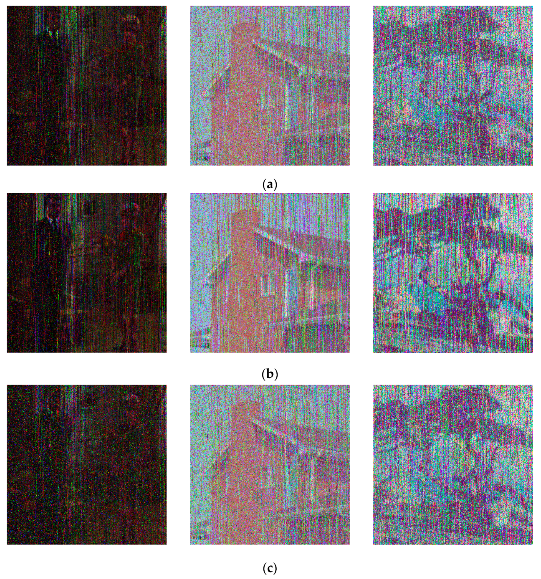
5.6. Noise Attacks Analysis

When the encrypted image is transmitted through the physical channel, it may be damaged by attackers [38]. Therefore, the cryptosystem should have the ability to resist noise attacks. That is, the cipher image after being attacked can still recover the information conveyed by the original image. In the experiment, we added Gaussian noise, Salt and pepper noise, and Speckle noise to the three cipher images in Figure 6b. As displayed in Figure 11, the decrypted images can still be successfully identified after being assaulted.

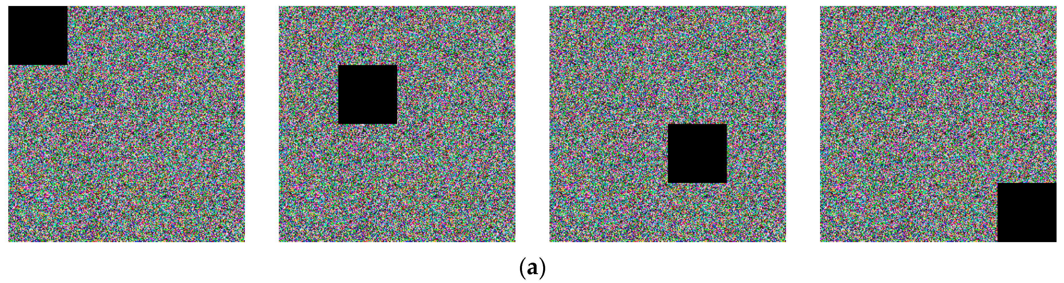
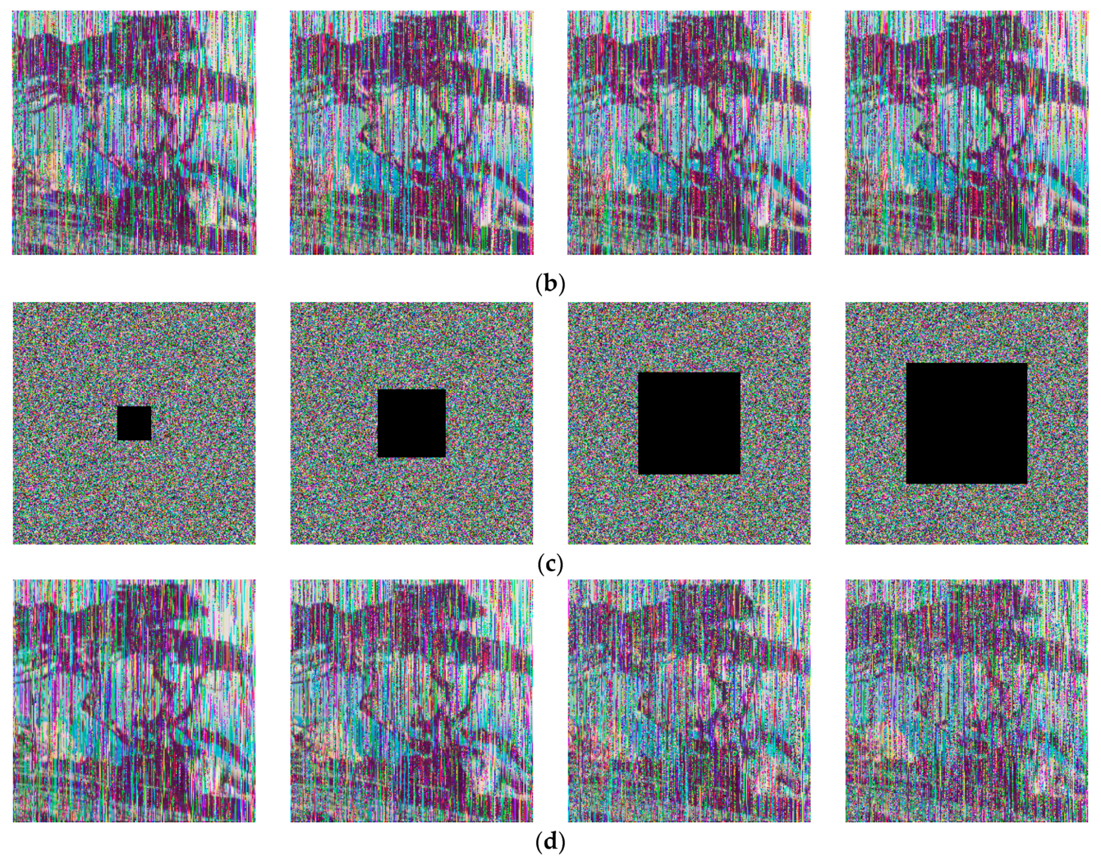
5.7. Data Loss Attack

A preeminent cryptosystem should withstand the cost of data loss during transmission and storage [39]. Similar to the test of noise attack, we also verified by decrypting the cipher image after data loss. Figure 12a,c reveals the data loss experiment on the cipher Tree image of different positions and sizes, respectively. It can be found from the corresponding decrypted images in Figure 12b,d that the Tree image after data leakage can still be recognized.

5.8. Differential Attack Analysis

The sensitivity to the plain image determines the ability of an algorithm to resist differential attacks. The measurement methods are the number of pixels change rate (NPCR) and unified average changing intensity (UACI) [40]. The formulas are as follows:

$$\mathrm{N}\mathrm{P}\mathrm{C}{\mathrm{R}}_{\mathrm{R},\mathrm{G},\mathrm{B}}=\frac{1}{\mathrm{M}\times \mathrm{N}}{\displaystyle \sum _{\mathrm{i}=1}^{\mathrm{M}}{\displaystyle \sum _{\mathrm{j}=1}^{\mathrm{N}}{\mathrm{E}}_{\mathrm{R},\mathrm{G},\mathrm{B}}(\mathrm{i},\mathrm{j})\times 100\mathrm{\%}}}$$

(23)

$$\mathrm{U}\mathrm{A}\mathrm{C}{\mathrm{I}}_{\mathrm{R},\mathrm{G},\mathrm{B}}=\frac{1}{\mathrm{M}\times \mathrm{N}}{\displaystyle \sum _{\mathrm{i}=1}^{\mathrm{M}}{\displaystyle \sum _{\mathrm{j}=1}^{\mathrm{N}}\frac{\left|{\mathrm{M}}_{\mathrm{R},\mathrm{G},\mathrm{B}}(\mathrm{i},\mathrm{j})-{{\mathrm{M}}^{\prime }}_{\mathrm{R},\mathrm{G},\mathrm{B}}(\mathrm{i},\mathrm{j})\right|}{255}\times 100\mathrm{\%}}}$$

(24)

where $\mathrm{M}$ and ${\mathrm{M}}^{\prime }$ are two cipher images whose plain images have only one different pixel. ${\mathrm{E}}_{\mathrm{R},\mathrm{G},\mathrm{B}}(\mathrm{i},\mathrm{j})$ is utilized to determine the distinction between two cipher images, which can be defined as:

$${\mathrm{E}}_{\mathrm{R},\mathrm{G},\mathrm{B}}(\mathrm{i},\mathrm{j})=\{\begin{array}{l}0,{\mathrm{M}}_{\mathrm{R},\mathrm{G},\mathrm{B}}(\mathrm{i},\mathrm{j})={{\mathrm{M}}^{\prime }}_{\mathrm{R},\mathrm{G},\mathrm{B}}(\mathrm{i},\mathrm{j})\\ 1,{\mathrm{M}}_{\mathrm{R},\mathrm{G},\mathrm{B}}(\mathrm{i},\mathrm{j})\ne {{\mathrm{M}}^{\prime }}_{\mathrm{R},\mathrm{G},\mathrm{B}}(\mathrm{i},\mathrm{j})\end{array}$$

(25)

In 2011, Wu et al. proposed more stringent standards of NPCR and UACI [41], which clearly demonstrates how high NPCR/UACI is, such that the encryption algorithm indeed has a high security level. The critical value ${\mathrm{N}}_{\mathsf{\alpha }}^{*}$ of significance level $\mathsf{\alpha }$ is calculated by

$${\mathrm{N}}_{\mathsf{\alpha }}^{*}=(\mathrm{F}-{\mathsf{\varphi }}^{-1}(\mathsf{\alpha })\sqrt{\frac{\mathrm{F}}{\mathrm{M}\mathrm{N}}})/(\mathrm{F}+1)$$

(26)

where ${\mathsf{\varphi }}^{-1}(\bullet )$ is the inverse cumulative density function (CDF) of the standard Normal distribution, and $\mathrm{F}$ denotes the largest supported pixel value compatible with the ciphertext image format. Assuming that the calculated value is greater than ${\mathrm{N}}_{\mathsf{\alpha }}^{*},$ then it can be proved to pass the test. The maximum ${\mathrm{N}}_{\mathsf{\alpha }}^{\ast -}$ and minimum ${\mathrm{N}}_{\mathsf{\alpha }}^{\ast +}$ of UACI can be computed according to Equation (27).

$$\{\begin{array}{l}{\mathrm{N}}_{\mathsf{\alpha }}^{\ast -}={\mathsf{\mu }}_{\mathrm{u}}-{\mathsf{\varphi }}^{-1}(\mathsf{\alpha }/2){\mathsf{\sigma }}_{\mathrm{u}}\\ {\mathrm{N}}_{\mathsf{\alpha }}^{\ast +}={\mathsf{\mu }}_{\mathrm{u}}+{\mathsf{\varphi }}^{-1}(\mathsf{\alpha }/2){\mathsf{\sigma }}_{\mathrm{u}}\end{array}$$

(27)

where ${\mathsf{\mu }}_{\mathrm{u}}=(\mathrm{F}+2)/(3\mathrm{F}+3)$, ${\mathsf{\sigma }}_{\mathrm{u}}^2=(\mathrm{F}+2)({\mathrm{F}}^2+2\mathrm{F}+3)/18{(\mathrm{F}+1)}^2\mathrm{M}\mathrm{N}\mathrm{F}$.

If the results of a scheme are between ${\mathrm{N}}_{\mathsf{\alpha }}^{\ast -}$ and ${\mathrm{N}}_{\mathsf{\alpha }}^{\ast +},$ it can be considered to pass the test.

Table 9. The theoretical values of number of pixels change rate (NPCR) and unified average changing intensity (UACI).

Size	NPCR (%)			UACI (%)
	${\mathbf{N}}_{0.05}^{\ast }$	${\mathbf{N}}_{0.01}^{\ast }$	${\mathbf{N}}_{0.001}^{\ast }$	$({\mathbf{N}}_{0.05}^{\ast -},{\mathbf{N}}_{0.05}^{\ast +})$	$({\mathbf{N}}_{0.01}^{\ast -},{\mathbf{N}}_{0.01}^{\ast +})$	$({\mathbf{N}}_{0.001}^{\ast -},{\mathbf{N}}_{0.001}^{\ast +})$
$256\times 256$	99.5693	99.5527	99.5341	(33.2824,33.6447)	(33.2255,33.7061)	(33.1594,33.7677)

reveals the theoretical values of NPCR and UACI at different significance levels for images of size $256\times 256$.

In our experiment, we encrypted plain images with the initial keys. Then, we randomly chose one pixel in each original image and changed them slightly. The modified images were encrypted with the same keys. After reckoning the two types of ciphers, it can be found that all the NPCR values in

Table 10. The actual values of NPCR for different color images.

Image	Calculated NPCR (%)			Theoretical NPCR (%)
	R	G	B	${\mathbf{N}}_{0.05}^{\ast }$	${\mathbf{N}}_{0.01}^{\ast }$	${\mathbf{N}}_{0.001}^{\ast }$
Couple	99.5956	99.6124	99.6185	Passed	Passed	Passed
House	99.6017	99.6268	99.5956	Passed	Passed	Passed
Tree	99.6094	99.6096	99.6129	Passed	Passed	Passed
Lena	99.6037	99.6128	99.5995	Passed	Passed	Passed
Peppers	99.5904	99.6246	99.6033	Passed	Passed	Passed
Baboon	99.5921	99.6109	99.6170	Passed	Passed	Passed
Lena in [35]	99.6357	99.6416	99.6224	-	-	-
Lena in [37]	99.6505	99.6444	99.6627	-	-	-
Lena in [42]	99.6300	99.5900	99.6700	-	-	-
Lena in [43]	99.6445	99.6353	99.6429	-	-	-
Peppers in [35]	99.5693	99.6435	99.6171	-	-	-
Peppers in [37]	99.6357	99.6158	99.6247	-	-	-
Baboon in [35]	99.6563	99.6428	99.6493	-	-	-
Baboon in [37]	99.6536	99.6078	99.6520	-	-	-
Baboon in [43]	99.6461	99.6628	99.6277	-	-	-

are greater than ${\mathrm{N}}_{\mathsf{\alpha }}^{*},$ and draw near to the ideal value of 99.6094%. Simultaneously, the UACI results for each image in

Table 11. The actual values of UACI for different color images.

Image	Calculated UACI (%)			Theoretical UACI (%)
	R	G	B	$({\mathbf{N}}_{0.05}^{\ast -},{\mathbf{N}}_{0.05}^{\ast +})$	$({\mathbf{N}}_{0.01}^{\ast -},{\mathbf{N}}_{0.01}^{\ast +})$	$({\mathbf{N}}_{0.001}^{\ast -},{\mathbf{N}}_{0.001}^{\ast +})$
Couple	33.5911	33.4298	33.4019	Passed	Passed	Passed
House	33.5739	33.4600	33.4721	Passed	Passed	Passed
Tree	33.4029	33.4018	33.4793	Passed	Passed	Passed
Lena	33.5056	33.4533	33.4719	Passed	Passed	Passed
Peppers	33.4634	33.5485	33.4818	Passed	Passed	Passed
Baboon	33.5139	33.4682	33.5363	Passed	Passed	Passed
Lena in [35]	33.5839	33.3954	33.4687	-	-	-
Lena in [37]	33.4462	33.4131	33.4399	-	-	-
Lena in [42]	33.4300	33.3900	33.5100	-	-	-
Lena in [43]	33.1147	30.5298	27.7471	-	-	-
Peppers in [35]	33.4317	33.5392	33.6326	-	-	-
Peppers in [37]	33.4570	33.4705	33.4423	-	-	-
Baboon in [35]	33.3687	33.5956	33.4528	-	-	-
Baboon in [37]	33.4753	33.5090	33.4176	-	-	-
Baboon in [43]	29.8421	28.1446	30.7024	-	-	-

are within the theoretical interval. Thus, the algorithm can effectively resist differential attacks.

5.9. Time and Computational Complexity Analysis

Time and speed analysis is also a critical measurement feature for an encryption algorithm. Thus, the security of a scheme cannot be at the expense of increasing time consumption. The time costs of images with different sizes were measured separately, and the results are listed in

Table 12. The encryption time and speed values for images with different sizes.

Image Size	Time (s)	Speed (bit/s)
$256\times 256$	0.4557	1091702.01
$512\times 512$	1.7383	1048478.39
$1024\times 1024$	6.4518	1127884.25
$256\times 256$ image in [31]	0.4862	-
$256\times 256$ image in [40]	1.85	-
$256\times 256$ image in [44]	1.32	-
$512\times 512$ image in [40]	3.76	-
$1024\times 1024$ image in [40]	26.34	-

. Obviously, the encryption time of our scheme is less than that of some recent encryption algorithms.

Ulteriorly, we will discuss the computational complexity of our scheme. At the outset, the generation process of the key streams made the computational complexity become $\mathsf{\Theta }(4\times \mathrm{m}\times \mathrm{n})$. Afterwards, the rows and columns of the three components R, G, and B were simultaneously cyclically shifted twice so that the computational complexity changed to $\mathsf{\Theta }(16\times \mathrm{m}\times \mathrm{n})$. Besides, the bit-level operations do not affect the complexity, hence the computational complexity of this paper is $\mathsf{\Theta }(16\times \mathrm{m}\times \mathrm{n})$.

6. Conclusions

In this paper, we devise a novel 1D chaotic map LFHCM with increased parameter space. The simulation results exhibit that the LFHCM has better chaotic properties than congeneric chaotic maps. In addition, combining LFHCM with a 4D hyperchaotic system, we also excogitate a color image encryption scheme based on tweak-cube theory. On the one hand, the secondary key streams updated by the plain image guarantee that the image withstands known-plaintext attack and chosen-plaintext attack. On the other hand, fast disorganizing at the bit-level and pixel-level allows our solution to be applied in crucial scenarios for real-time communication, such as telemedicine, authentication, and so forth. Compared with some state-of-arts, our work has achieved excellent encryption effects.

References

1. Wu, X.; Kan, H.; Kurths, J. A new color image encryption scheme based on DNA sequences and multiple improved 1D chaotic maps. Appl. Soft Comput. 2015, 37, 24–39. [Google Scholar] [CrossRef]
2. Li, C.; Luo, G.; Ke, Q.; Li, C. An image encryption scheme based on chaotic tent map. Nonlinear Dyn. 2017, 87, 127–133. [Google Scholar] [CrossRef]
3. Ye, G.; Chen, P.; Huang, X.; Mei, Q. An efficient pixel-level chaotic image encryption algorithm. Nonlinear Dyn. 2018, 94, 1–12. [Google Scholar] [CrossRef]
4. Kaur, M.; Kumar, V. Efficient image encryption method based on improved Lorenz chaotic system. Electron. Lett. 2018, 54, 562–564. [Google Scholar] [CrossRef]
5. Wang, X.; Çavuşoğlu, Ü.; Kacar, S.; Akgul, A.; Pham, V.-T.; Jafari, S.; Alsaadi, E.F.; Nguyen, Q.X. S-Box Based Image Encryption Application Using a Chaotic System without Equilibrium. Appl. Sci. 2019, 9, 781. [Google Scholar] [CrossRef]
6. Zhou, N.; Li, H.; Di, W.; Pan, S.; Zhou, Z. Image compression and encryption scheme based on 2D compressive sensing and fractional Mellin transform. Opt. Commun. 2015, 343, 10–21. [Google Scholar] [CrossRef]
7. Liu, X.; Mei, W.; Du, H. Optical image encryption based on compressive sensing and chaos in the fractional Fourier domain. J. Mod. Opt. 2014, 61, 1570–1577. [Google Scholar] [CrossRef]
8. Ye, G. A block image encryption algorithm based on wave transmission and chaotic systems. Nonlinear Dyn. 2014, 75, 417–427. [Google Scholar] [CrossRef]
9. Chai, X.L.; Zhu, C.J.; Yang, K.; Gao, Y.L. Block Image Encryption Scheme Based on Wave Transmission and Hyperchaotic Financial System. J. Chin. Comput. Syst. 2016, 37, 1329–1333. [Google Scholar]
10. Guesmi, R.; Farah, M.A.B.; Kachouri, A.; Samet, M. A novel chaos-based image encryption using DNA sequence operation and Secure Hash Algorithm SHA-2. Nonlinear Dyn. 2016, 83, 1–14. [Google Scholar] [CrossRef]
11. Guesmi, R.; Farah, M.A.B.; Kachouri, A.; Samet, M. Hash key-based image encryption using crossover operator and chaos. Multimed. Tools Appl. 2016, 75, 4753–4769. [Google Scholar] [CrossRef]
12. Yong, Z. The image encryption algorithm based on chaos and DNA computing. Multimed. Tools Appl. 2018, 77, 21589–21615. [Google Scholar]
13. Chai, X.; Chen, Y.; Broyde, L. A novel chaos-based image encryption algorithm using DNA sequence operations. Opt. Lasers Eng. 2017, 88, 197–213. [Google Scholar] [CrossRef]
14. Wang, X.; Zhang, H.L. A novel image encryption algorithm based on genetic recombination and hyper-chaotic systems. Nonlinear Dyn. 2016, 83, 333–346. [Google Scholar] [CrossRef]
15. Chen, J.X.; Zhu, Z.L.; Chong, F.; Zhang, L.B.; Zhang, Y. An efficient image encryption scheme using lookup table-based confusion and diffusion. Nonlinear Dyn. 2015, 81, 1151–1166. [Google Scholar] [CrossRef]
16. Kumar, M.; Iqbal, A.; Kumar, P. A new RGB image encryption algorithm based on DNA encoding and elliptic curve Diffie-Hellman cryptography. Signal Process. 2016, 125, 187–202. [Google Scholar] [CrossRef]
17. Pareek, N.K.; Patidar, V.; Sud, K.K. Image encryption using chaotic logistic map. Image Vis. Comput. 2006, 24, 926–934. [Google Scholar] [CrossRef]
18. Singh, N.; Sinha, A. Optical image encryption using Hartley transform and logistic map. Opt. Commun. 2009, 282, 1104–1109. [Google Scholar] [CrossRef]
19. Wang, X.; Lin, T.; Xue, Q. A novel colour image encryption algorithm based on chaos. Signal Process. 2012, 92, 1101–1108. [Google Scholar] [CrossRef]
20. Yue, W.; Yang, G.; Jin, H.; Noonan, J.P. Image encryption using the two-dimensional logistic chaotic map. J. Electron. Imaging 2012, 21, 3014. [Google Scholar]
21. Zhou, Y.; Long, B.; Chen, C.L.P. A new 1D chaotic system for image encryption. Signal Process. 2014, 97, 172–182. [Google Scholar] [CrossRef]
22. Hua, Z.; Zhou, Y.; Pun, C.M.; Chen, C.L.P. 2D Sine Logistic modulation map for image encryption. Inf. Sci. 2015, 297, 80–94. [Google Scholar] [CrossRef]
23. Pak, C.; Huang, L. A new color image encryption using combination of the 1D chaotic map. Signal Process. 2017, 138, 129–137. [Google Scholar] [CrossRef]
24. Hanis, S.; Amutha, R. A fast double-keyed authenticated image encryption scheme using an improved chaotic map and a butterfly-like structure. Nonlinear Dyn. 2019, 95, 421–432. [Google Scholar] [CrossRef]
25. Lu, J.A.; Wu, X.; Lü, J.; Kang, L. A new discrete chaotic system with rational fraction and its dynamical behaviors. Chaos Solitons Fractals 2004, 22, 311–319. [Google Scholar] [CrossRef]
26. Zhu, S.; Wang, G.; Zhu, C. A Secure and Fast Image Encryption Scheme Based on Double Chaotic S-Boxes. Entropy 2019, 21, 790. [Google Scholar] [CrossRef]
27. Pincus, S. Approximate entropy (ApEn) as a complexity measure. Chaos 1995, 5, 110–117. [Google Scholar] [CrossRef]
28. He, J.; Cai, J. Design of a New Chaotic System Based on Van Der Pol Oscillator and Its Encryption Application. Mathematics 2019, 7, 743. [Google Scholar] [CrossRef]
29. Guangzhou and China. A new hyperchaotic system and its adaptive tracking control. Acta Phys. Sin. 2012, 61, 273–335. [Google Scholar]
30. Wang, X.Y.; Li, P.; Zhang, Y.Q.; Liu, L.Y.; Zhang, H.; Wang, X. A novel color image encryption scheme using DNA permutation based on the Lorenz system. Multimed. Tools Appl. 2018, 77, 6243–6265. [Google Scholar] [CrossRef]
31. Sun, S. A novel hyperchaotic image encryption scheme based on DNA encoding, pixel-level scrambling and bit-level scrambling. IEEE Photonics J. 2018, 10. [Google Scholar] [CrossRef]
32. Enayatifar, R.; Sadaei, H.J.; Abdullah, A.H.; Lee, M.; Isnin, I.F. A novel chaotic based image encryption using a hybrid model of deoxyribonucleic acid and cellular automata. Opt. Lasers Eng. 2015, 71, 33–41. [Google Scholar] [CrossRef]
33. Xie, Y.; Yu, J.; Guo, S.; Ding, Q.; Wang, E. Image Encryption Scheme with Compressed Sensing Based on New Three-Dimensional Chaotic System. Entropy 2019, 21, 819. [Google Scholar] [CrossRef]
34. Cicek, I.; Pusane, A.E.; Dundar, G. A novel design method for discrete time chaos based true random number generators. Integr. VLSI J. 2014, 47, 38–47. [Google Scholar] [CrossRef]
35. Liu, H.; Kadir, A.; Sun, X. Chaos-based fast color image encryption scheme with true random number keys from environmental noise. IET Image Process. 2017, 11, 324–332. [Google Scholar] [CrossRef]
36. Parvaz, R.; Zarebnia, M. A combination chaotic system and application in color image encryption. Opt. Laser Technol. 2018, 101, 30–41. [Google Scholar] [CrossRef] [Green Version]
37. Niyat, A.Y.; Moattar, M.H.; Torshiz, M.N. Color image encryption based on hybrid hyper-chaotic system and cellular automata. Opt. Lasers Eng. 2017, 90, 225–237. [Google Scholar] [CrossRef]
38. Liu, H.; Kadir, A. Asymmetric color image encryption scheme using 2D discrete-time map. Signal Process. 2015, 113, 104–112. [Google Scholar] [CrossRef]
39. Wang, L.; Song, H.; Ping, L. A novel hybrid color image encryption algorithm using two complex chaotic systems. Opt. Lasers Eng. 2016, 77, 118–125. [Google Scholar] [CrossRef]
40. Wu, X.; Zhu, B.; Hu, Y.; Ran, Y. A Novel Color Image Encryption Scheme Using Rectangular Transform-Enhanced Chaotic Tent Maps. IEEE Access 2017, 5, 6429–6436. [Google Scholar]
41. Wu, Y. NPCR and UACI Randomness Tests for Image Encryption. Cyber J. J. Sel. Areas Telecommun. 2011, 1, 31–38. [Google Scholar]
42. Wang, X.; Zhao, Y.; Zhang, H.; Guo, K. A novel color image encryption scheme using alternate chaotic mapping structure. Opt. Lasers Eng. 2016, 82, 79–86. [Google Scholar] [CrossRef]
43. Suri, S.; Vijay, R. A synchronous intertwining logistic map-DNA approach for color image encryption. J. Ambient Intell. Humaniz. Comput. 2019, 10, 2277–2290. [Google Scholar] [CrossRef]
44. Xu, L.; Li, Z.; Li, J.; Hua, W. A novel bit-level image encryption algorithm based on chaotic maps. Opt. Lasers Eng. 2016, 78, 17–25. [Google Scholar] [CrossRef]
Figure 1. The bifurcation graphs of the (a) Logistic-Fraction hybrid chaotic map (LFHCM); (b) Logistic map; (c) Fraction map.
Applsci 09 04854 g001
Figure 2. The Lyapunov exponents of the (a) LFHCM; (b) Logistic map; (c) Fraction map.
Applsci 09 04854 g002
Figure 3. The phase trajectories of the (a) x, y plane; (b) x, z plane; (c) x, w plane; (d) y, z plane; (e) y, w plane; (f) x, y, z space.
Applsci 09 04854 g003
Figure 4. Schematic diagram of cyclic shifting in all directions.
Applsci 09 04854 g004
Figure 5. Flowchart of the encryption scheme.
Applsci 09 04854 g005
Figure 6. Encryption results: (a) the original images; (b) the encrypted images; (c) the decrypted images.
Applsci 09 04854 g006
Figure 7. (a) The cipher images with a small change to initial value x10; (b) the pixel-by-pixel differences between (a) and Figure 6b.
Applsci 09 04854 g007
Figure 8. Histograms of the (a) plain images in Figure 6a; (b) cipher images in Figure 6b.
Applsci 09 04854 g008
Figure 9. Correlation coefficients of plain Tree image in each direction: (a) R channel; (b) G channel; (c) B channel.
Applsci 09 04854 g009
Figure 10. Correlation coefficients of cipher Tree image in each direction: (a) R channel; (b) G channel; (c) B channel.
Applsci 09 04854 g010
Figure 11. Decrypted images with (a) Gaussian noise; (b) salt & pepper noise; (c) speckle noise.
Applsci 09 04854 g011
Figure 12. (a) Cipher images with lost data at different locations; (b) decrypted images of (a); (c) cipher images with different sizes of data loss; (d) decrypted images of (c).
Applsci 09 04854 g012aApplsci 09 04854 g012b