1. Introduction
As a major task of condition-based maintenance (CBM), health prognostics can predictively maintain equipment, improve the reliability of the machinery and prevent catastrophic consequences [
1,
2,
3,
4,
5]. The main purpose of health prognostics is to explore the on-going degradation law for the device by feature extraction of the device-related data, and then predict the remaining useful life (RUL) [
6]. Consequently, RUL prediction has received more and more attention from academia and industry.
RUL prediction methods can be classified into two categories: model-driven methods and data-driven methods. The model-driven methods aim to derive the degradation process of a machine by setting up mathematical or physical models [
7]. With the commonly used models such as the Markov process model, the Winner process model and the Gaussian mixture model, the RUL can be predicted [
8]. However, such methods rely on robust physical or mathematical models, which are difficult to obtain owing to the complex environment [
9]. Data-driven methods establish the relationship between the acquired data and RUL through data mining, which can be more accurate with the real-time monitoring data. In recent years, a number of effective data-driven algorithms have been proposed and achieved good results, mainly including: neural networks [
10], support vector regression (SVR) [
11] and gaussian process regression (GPR) [
12].
Generally, data-driven methods consist of three stages: data acquisition, health indicator (HI) construction and RUL prediction [
13,
14,
15,
16]. By learning the deterioration curve of HIs, the time it takes for the current HI to reach the pre-set failure threshold (i.e., RUL) is estimated. Louen et al. [
17] proposed a new health indicator creation approach using binary support vector machine classifier and calculated the RUL through an identified Weibull function. Guo et al. [
6,
18] applied neural networks to the construction of health indicators and the RUL was obtained by the particle filter. Malhotra et al. [
19] constructed a long short-term memory-based encoder-decoder (LSTM-ED) scheme to obtain an unsupervised health indicator (HI).
Generally, the prediction accuracy of RUL is seriously affected by the quality of the constructed HIs [
20,
21]. The current HI construction methods are perplexed by different amplitude ranges of statistical features, which leads to unifying the failure threshold difficultly under different working conditions [
9,
18]. In addition, as shown in
Figure 1a, prediction methods based on HIs depend on long-term tracking of equipment from the initial to the current time, which is impractical in some cases.
Hence, some scholars have paid attention to the time window (TW)-based RUL prediction method and have begun to directly establish the correlation between the sensor signals and RUL. Lim et al. [
22] developed a machine learning framework with a moving time window to determine the RUL of aircraft engines. Zhang et al. [
23] used a fixed time window to predict the RUL of aircraft engines. As depicted in
Figure 1b, this method can start sampling at any time when the equipment is running, obtain the data from
to
, and the RUL at
can be predicted directly according to these data. The key issue of these methods is to establish the mapping between the original signal and the RUL.
Recently, deep learning has made remarkable achievements in the fields of image recognition, speech recognition and unmanned driving [
24,
25]. Deep learning is characterized by the deep network architecture where multiple layers are stacked in the network to fully capture the representative information from the raw input data [
26]. Therefore, as a powerful tool, deep learning shows its great potential in establishing the correlation between the original signals and the RUL. Lim et al. [
22] created a multilayer neural network as the deep learning algorithm to build the correlation between signal characteristics and RUL. Zhang et al. [
23] proposed a multi-objective deep belief networks ensemble (MODBNE) method for RUL prediction, which employs a multi-objective evolutionary algorithm integrated with the traditional deep belief networks (DBN) training technique to evolve multiple DBNs simultaneously subject to accuracy and diversity as two conflicting objectives. Within the deep learning architecture, convolutional neural network (CNN) is further applied in this study because of its excellent feature extraction ability in the face of variable and complex signals [
27]. Babu et al. [
28] firstly applied CNNs to the field of RUL prediction and incorporated automated feature learning from the raw sensor signals in a systematic way. Li et al. [
27] established a deep CNN model and conducted a preliminary exploration of the depth of the networks on RUL prediction. While CNNs have shown great potential in prognostics, there are still few applications of CNN in RUL prediction.
In this paper, a novel CNN is presented. The kernel module composed of multiple convolutional kernels was proposed for feature extraction. This module was derived from the inception network proposed by Szegedy et al. [
25]. Compared with the module used in the inception network, the feature extraction of the convolution kernel was in the time dimension, which reduced the parameters of the module and transfers the application in the image field to prognostics. The relationship between the raw signals and the RUL could be established through the learning process. The RUL was calculated according to the new vector of input signals.
In this study, we used the C-MAPSS dataset provided by NASA for the RUL prediction of aircraft engines [
29]. The engine is the key component of the aircraft and there is always a pressing need to develop new approaches to better evaluate the engine performance degradation and estimate the remaining useful life [
30]. The proposed network showed its superiority compared with the state-of-art methods on the same dataset. Our attempt was a useful exploration for implementing the RUL prediction on the unexpected events and provides the possibility to transfer the proposed method in a simpler scenario.
This remainder of the paper is organized as follows. The proposed CNN is given in
Section 2, which illustrates the proposed architecture and the main scheme of the kernel module used in the convolution layers. The experimental results of the proposed model compared with different depths, time windows, optimization algorithms and other state-of-the-art methods are given in
Section 3.
Section 4 summarizes the conclusions of this work.
2. The Proposed Deep CNN Architecture
As presented in
Figure 2, the deep learning architecture proposed consisted of the convolution layers, pooling layers and the fully-connected layer. Firstly, the normalized sensor data with the time window was directly used as input to the CNN, and then the feature maps were increased. Secondly, the convolution layer which was characterized by the kernel module was utilized for feature extraction and the down sampling scheme was operated by the pooling layer. Thirdly, the dimension reduction was performed before the fully connected layer, and then the feature mapping was implemented at the fully connected layer.
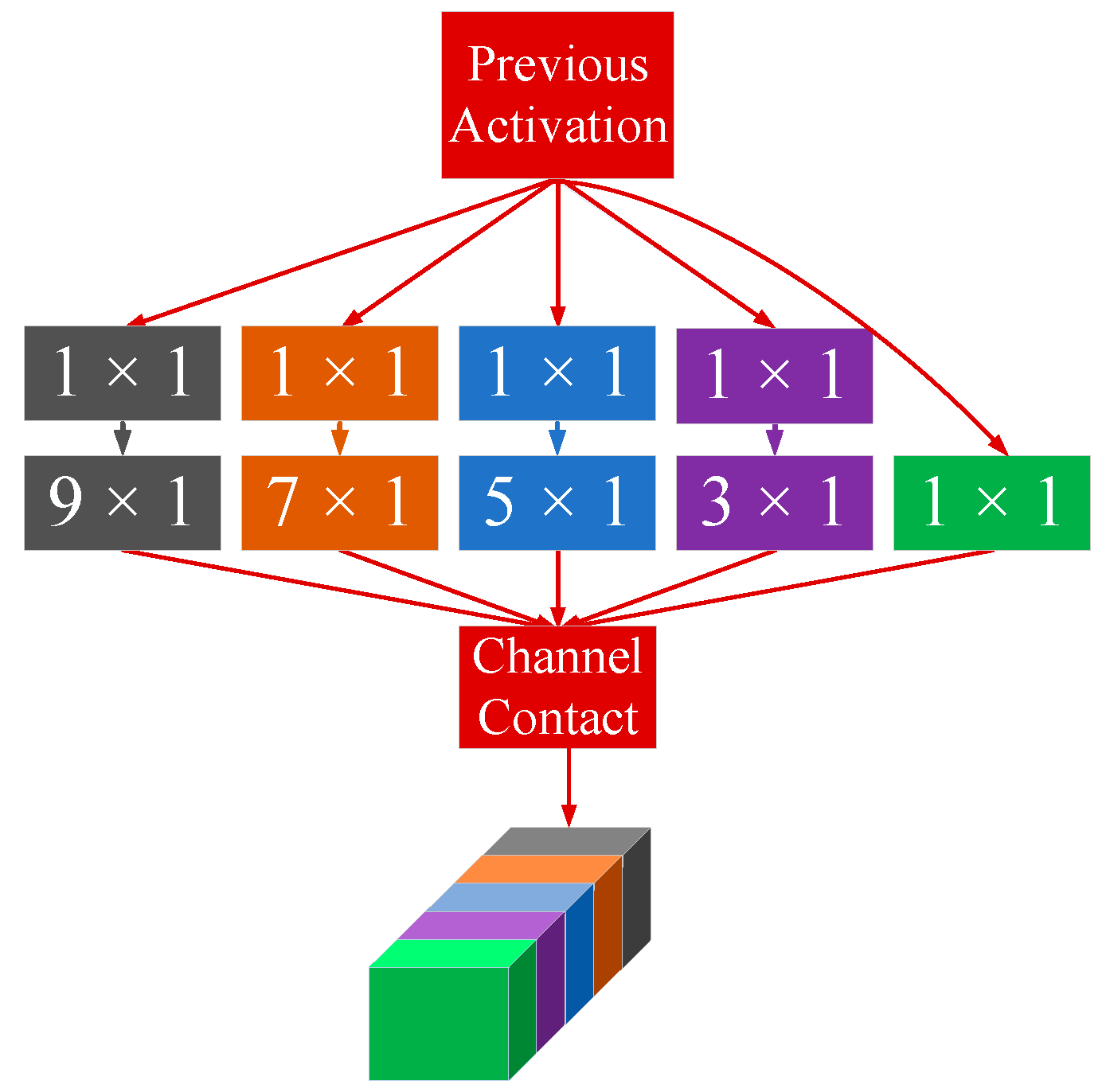
2.1. The Kernel Module
The CNN previously used in prognostics contains only convolution kernels of the same size. However, the field of vision extracted by a small-sized kernel could be smaller, and a larger-sized kernel may ignore the details. Hence, different sizes of kernels can be used in each convolution layer to let the CNN automatically learn to select the size of the kernel. The selected kernels are one-dimensional because feature extraction is mainly performed in the time dimension. The size of the kernel in the module should be adjusted according to the size of the input data, which means the size of the kernel cannot be larger than the size of the input data for the module in the time dimension. Each convolution layer is characterized by the kernel module which is composed of kernels with different sizes. The padding method was “SAME”. The kernel module is illustrated in
Figure 3.
The
Lth layer is assumed to be the convolution layer which can be denoted as:
where
is the
jth feature map of the output on the
Lth layer,
is the
ith feature map of the output on the
L-1th layer,
is all the feature maps of the output on the
L-1th layer,
is the
jth kernel on the
Lth layer,
is the
jth bias on the
Lth layer.
The 1 × 1 convolution kernel can be used in front of the other kernels as the bottleneck to directly reduce the computational burden of the convolution layer, which is explained in the next subsection.
2.2. The 1 × 1 Kernels
The 1 × 1 convolution kernel was proposed firstly by Szegedy et al. [
25], which has two functions. Firstly, by adding the 1 × 1 kernels in front of other kernels in the kernel module, the computational cost can be reduced. The total number of multipliers is the number of multipliers that need to be calculated for each of output values times the number of output values. As illustrated in
Figure 4, two techniques are given for inputting
and outputting
, the first method is to use only
convolution kernels, and an alternative architecture is to use the
convolution kernels and then the
convolution kernels.
The total number of multipliers for the first technique
and the second technique
can be calculated by
where
represents the number of feature maps after the
kernels.
If
, then
hence, the computational load can be reduced.
The second function of the 1 × 1 kernel is to change the number of feature maps and implement linear combination of multiple feature maps. The input data is processed by the 1 × 1 kernel, and then the number of the feature maps is increased, providing the convolution layer with the data for feature extraction. In addition, the 1 × 1 convolution kernel is used for dimension reduction before the fully-connected layer, which can further enhance the correlation between the extracted features and RUL.
2.3. The Proposed Network
The proposed deep convolution neural network is shown in
Figure 5. The depth of the network is determined by the convolution-pooling layer or convolution layer. The pooling layer is used to reduce the dimensions and does not need to perform complex matrix operations or learn any parameters. The size of the kernel in the pooling layer is 2 × 1, and the stride is 2 × 1. The pooling method is ‘VALID’ max pooling and the size of input data will be halved in the time dimension through the pooling layer. Finally, the fully-connected layer maps the features learned by the CNN to the output through converting three-dimensional data into one-dimensional.
The input data is three-dimensional and is expressed by T × S × F, where T is the length of the TW, S is the sensor data and F is the number of feature map (the input data contains only one feature map). The normalized data for T consecutive time cycles is directly used as input to the CNN. As the depth of the model increases, the number of convolution kernels after the 1 × 1 kernels in each layer is doubled until the input of the Lth layer is less than six in the time dimension, and the pooling layer will no longer be included in the layer and subsequent layers. If the pooling layer for the input data less than six is used again, only the 1 × 1 convolution kernel can be used in the next layer, which is only an increase in the number of feature maps rather than feature extraction. The number and size of the convolution kernels in the subsequent layers will be the same as the Lth layer. Before other kernels, the number of 1 × 1 kernels is half that of other kernels to satisfy Equation (3), while the first layer is different. This is because the number of the initial 1 × 1 kernels before the first convolution-pooling layer is half of other kernels in the first layer, so the number of the 1 × 1 kernels before other kernels is set to one quarter of other kernels in the first layer as the bottleneck to reduce the parameters. Note that, the maximum size of the kernel in each layer should be less than or equal to the time dimension of the input data in that layer.
Here is a concrete example, when the TW size was set to 30, the number of different kernels is presented in
Table 1. Due to the dimensionality reduction of the pooling layer, the input size of the third layer was 7 × S × 160, so the kernel module in this layer removed the 9 × 1 kernels. Similarly, only 1 × 1 and 3 × 1 convolution kernels were used in the fourth and subsequent last layers, and no pooling layers were added.
4. Conclusions
The traditional health indicator-based methods need the long-term tracking of the signals, which are laborious and time-consuming. A novel CNN based on the time window was proposed to tackle this issue. Additionally, the kernel module was constructed, which can let the network learn to select the kernels automatically. The effectiveness of the proposed network was demonstrated using the C-MAPSS dataset. The main contributions of this paper are as follows:
(1) The raw industrial sensor signals were standardized and transmitted to the network for RUL prediction without long-term tracking and constructing HIs that relied on signal processing expertise.
(2) A novel kernel module composed of one-dimensional convolutional kernels of different sizes was proposed for feature extraction in time series.
(3) The 1×1 convolutional kernel was introduced to handle the multiple channels in the kernel module.
However, some limitations still existed in the presented methods. For example, the networks for each sub-dataset were trained and evaluated separately. Besides, the C-MAPSS dataset was created by simulation models in controlled environments. The real world has many uncontrollable events, which should be considered further.


