Exposure Bracketing Techniques for Camera Document Image Enhancement

Abstract

Capturing document images using digital cameras in uneven lighting conditions is challenging, leading to poorly captured images, which hinders the processing that follows, such as Optical Character Recognition (OCR). In this paper, we propose the use of exposure bracketing techniques to solve this problem. Instead of capturing one image, we used several images that were captured with different exposure settings and used the exposure bracketing technique to generate a high-quality image that incorporates useful information from each image. We found that this technique can enhance image quality and provides an effective way of improving OCR accuracy. Our contributions in this paper are two-fold: (1) a preprocessing chain that uses exposure bracketing techniques for document images is discussed, and an automatic registration method is proposed to find the geometric disparity between multiple document images, which lays the foundation for exposure bracketing; (2) several representative exposure bracketing algorithms are incorporated in the processing chain and their performances are evaluated and compared.

1. Introduction

Camera document images provide many possibilities for further processing (for example, Optical Character Recognition (OCR)) if the captured image quality is good [1]. However, the captured image quality may vary depending on the imaging conditions. One difficult case where the captured image is far from ideal is when there is uneven lighting. In this case, some regions in the captured image are over-exposed while other regions are under-exposed. Though adaptive imaging processing techniques such as the Sauvola binarization method have been proposed to solve this problem [2], when the uneven lighting is severe, the lost textual information due to over-exposure or under-exposure cannot be retrievable as this information is not captured by the camera’s sensor.

In this paper, we considered using an exposure bracketing technique to solve the uneven lighting problem. Exposure bracketing is a technique of formulating one single image by combining multiple images of the same scene but with different exposure times [3]. In the uneven lighting environment, irradiance across the scene varies greatly, leading to over-exposed imaging areas and under-exposed imaging areas regardless of the set exposure time. These over-exposed and under-exposed areas carry less information than the same areas when they are well-exposed. In order to capture details about an entire scene, it is necessary to capture images at multiple exposures. In doing so, the over-exposed or under-exposed image patches in one image can always find their corresponding patches in another image where the imaging area was well-exposed.

Generating images with different exposure times is becoming much easier nowadays because more and more consumer cameras or smart phones allow the user to manually adjust the exposure time when capturing. Document images that are captured with different exposure times show different characteristics. Figure 1 shows such an example where three exposure images are generated for the same document. It is obvious that these images contain complementary information. For example, the left-bottom part in Figure 1a is under-exposed, but that area is well-exposed in Figure 1c; the left central part in Figure 1a is well-exposed, while that area is over-exposed in Figure 1c. These three images are captured with the Huawei Phone P20 in the same lighting condition and for the under-exposed case, the exposure time is 1/800 s; for the well-exposed case, the exposure time is 1/320 s; and for the over-exposed case, the exposure time is 1/40 s. Intuition tells us that we can generate a better image by selecting the best image patches or pixels from these three images.

In the following sections, first of all we will have a technical overview of exposure bracketing techniques. After that, we will disclose a registration method that particularly suits document image exposure bracketing. Then, we will select four representative exposure bracketing algorithms and use them in the context of document image exposure bracketing. In the experiment section, we will compare these methods and see how different exposure bracketing methods help to increase OCR accuracy and finally, we will draw our conclusion as well as directions for future research.

2. Technical Overview of Exposure Bracketing Techniques

Exposure bracketing techniques can be divided into two groups [3]. The first group method is closely related to tone mapping. The basic idea behind it is to create a high dynamic range radiance map, first by combining all the low dynamic range (LDR) images (that is, images with different exposures) and after that, a mapping function is employed to transform the high dynamic range radiance map to a high dynamic range (HDR) image. For more details on HDR image generation, please refer to [3]. This processing chain is shown in Figure 2.

In Figure 2, image registration is employed before mapping LDR image pixel values on the radiance map. The reason why image registration is needed is because when generating the multiple exposure images, there are always geometric disparities between them. Therefore, it is necessary to align them in a common coordinate system where the same pixels in different images share the same coordinate.

The second category of exposure bracketing techniques is called exposure fusion, as shown in Figure 3. Compared to the tone mapping method, this method does not generate a radiance map based on the input of multiple exposure images. Instead, it first selects or calculates a weighting factor for each pixel in multiple LDR images based on some quality criteria and then generates an HDR image by padding the selected pixel or weighted sum of pixels of multiple images. This method usually follows the following processing chain:

In the context of document image exposure bracketing, the literature we found is really limited. The only paper that discloses document image exposure bracketing techniques can be found in paper [4], where an adaptive image fusion was used. However, there are two limitations in this paper: (1) the author assumes that document images are captured with a fixed camera and hence there is no need to perform image registration. As we will discuss in the next section, projective distortion often happens when capturing document images and there are geometric disparities among the captured images. (2) The author discusses and compares different image fusion strategies, however tone mapping techniques are missing from their comparison. We think that it is necessary to incorporate tone mapping in the processing chain as it is one of the mainstream methods in exposure bracketing. It is true that there are several papers that discuss the document image registration problem. For example, in paper [5], the classic key point feature descriptor-based image registration method was combined with mobile phone sensor data such as the accelerometer and gyroscope sensor data to perform image mosaic reconstruction. However, their registration is more suitable for the image mosaic reconstruction purpose while the registration method that we used is more suitable for exposure bracketing.

As both categories of methods employ image registration as a preprocessing step, it is necessary to first find a proper image registration method in the context of document image exposure bracketing.

3. HDR Document Image Generation

3.1. Document Image Registration

The image registration problem has been intensively studied in remote sensing images, medical images, and camera images and very rarely, research can be found for document image registration. The most popular registration in the context of exposure bracketing is from [3], where a translational geometric model was employed to account for the geometric disparity between two images. However, we found that the translational model is not suitable for general camera document images.

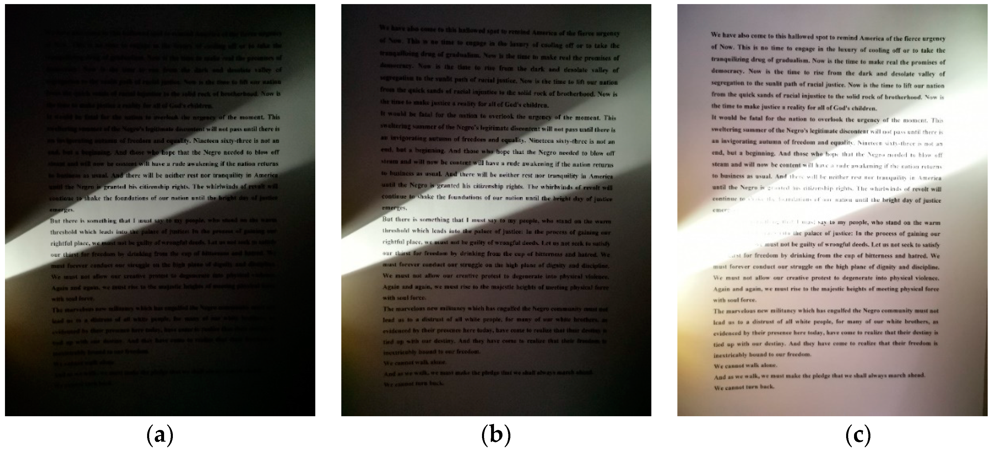
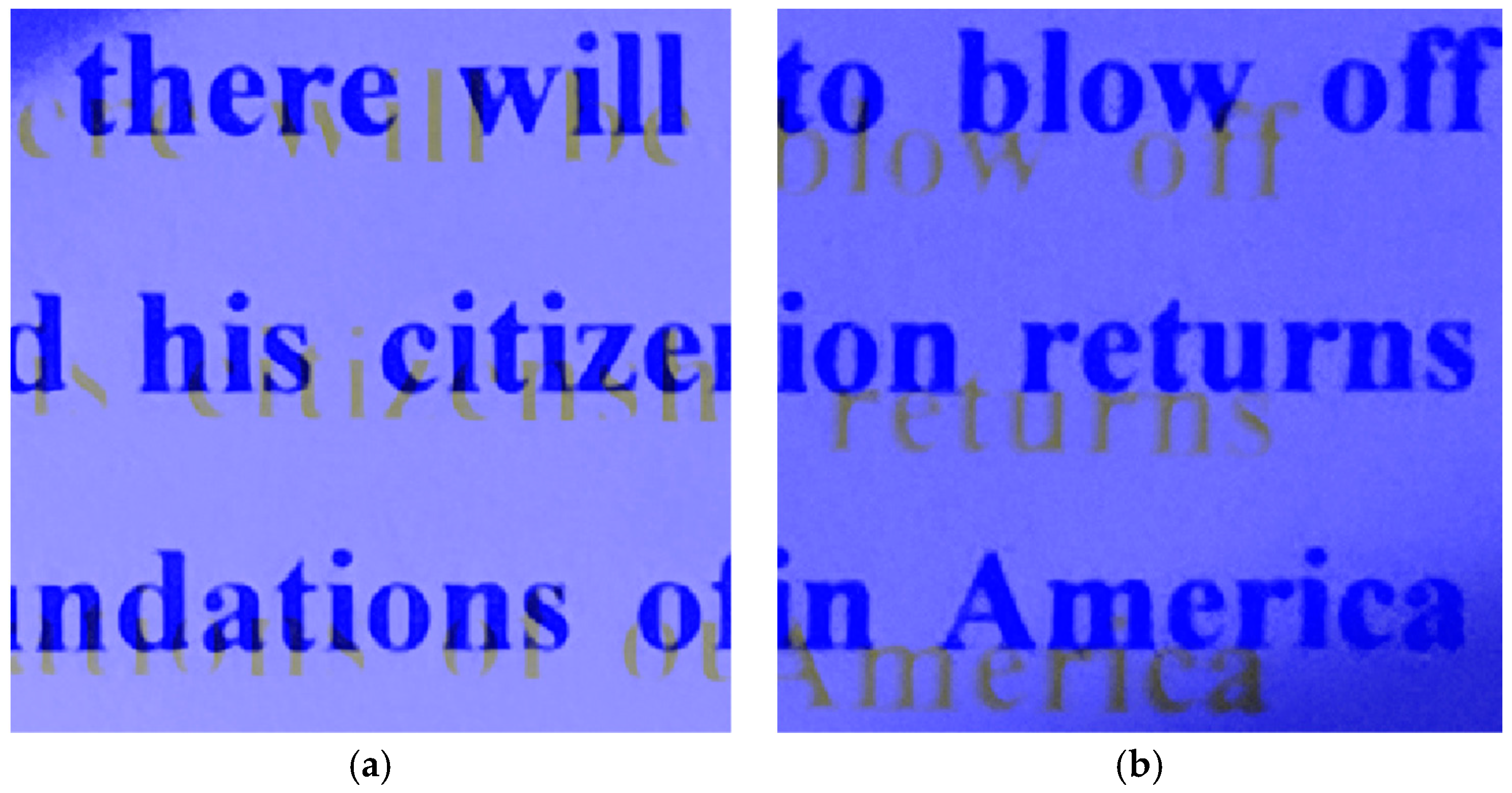
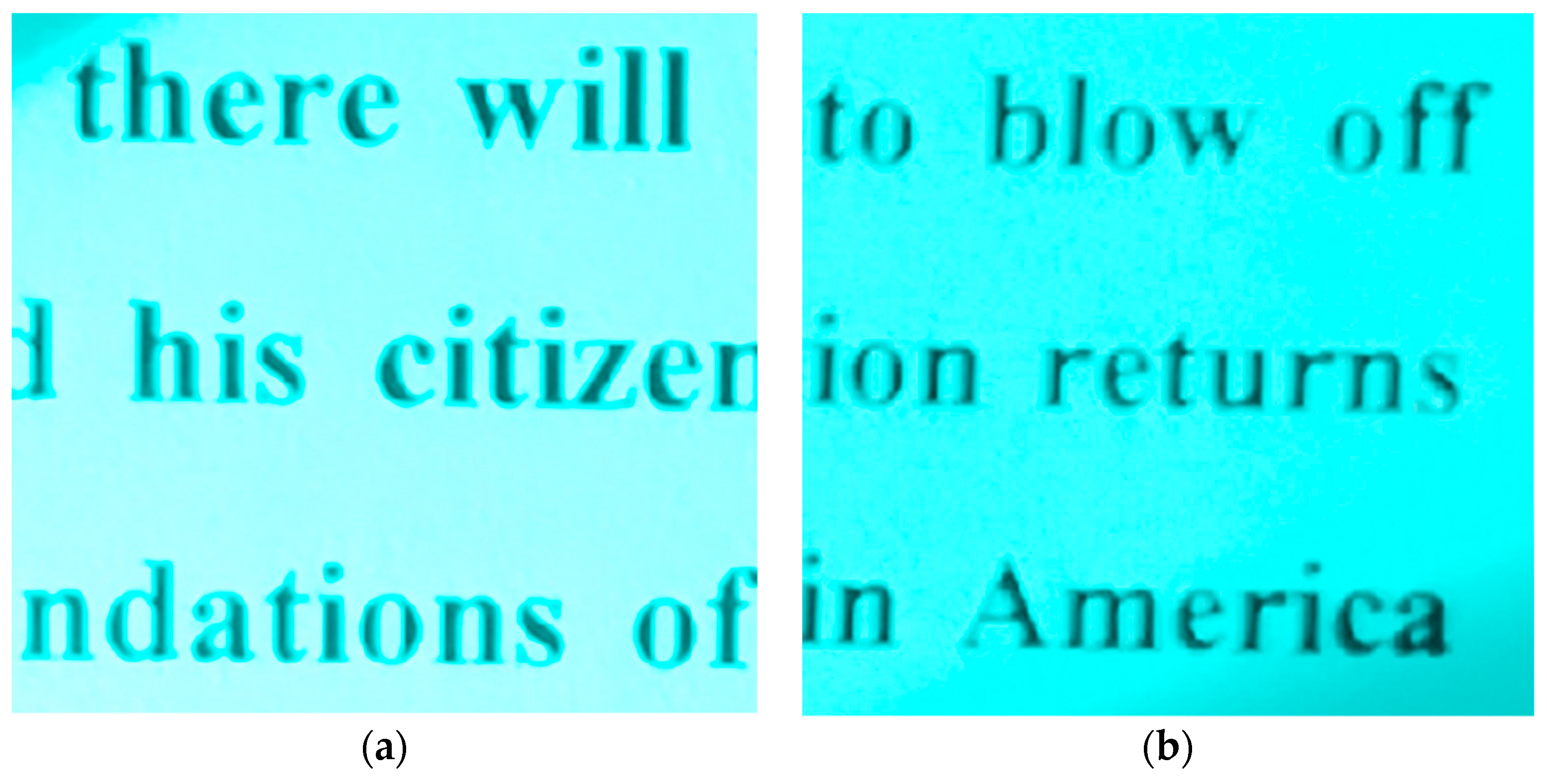
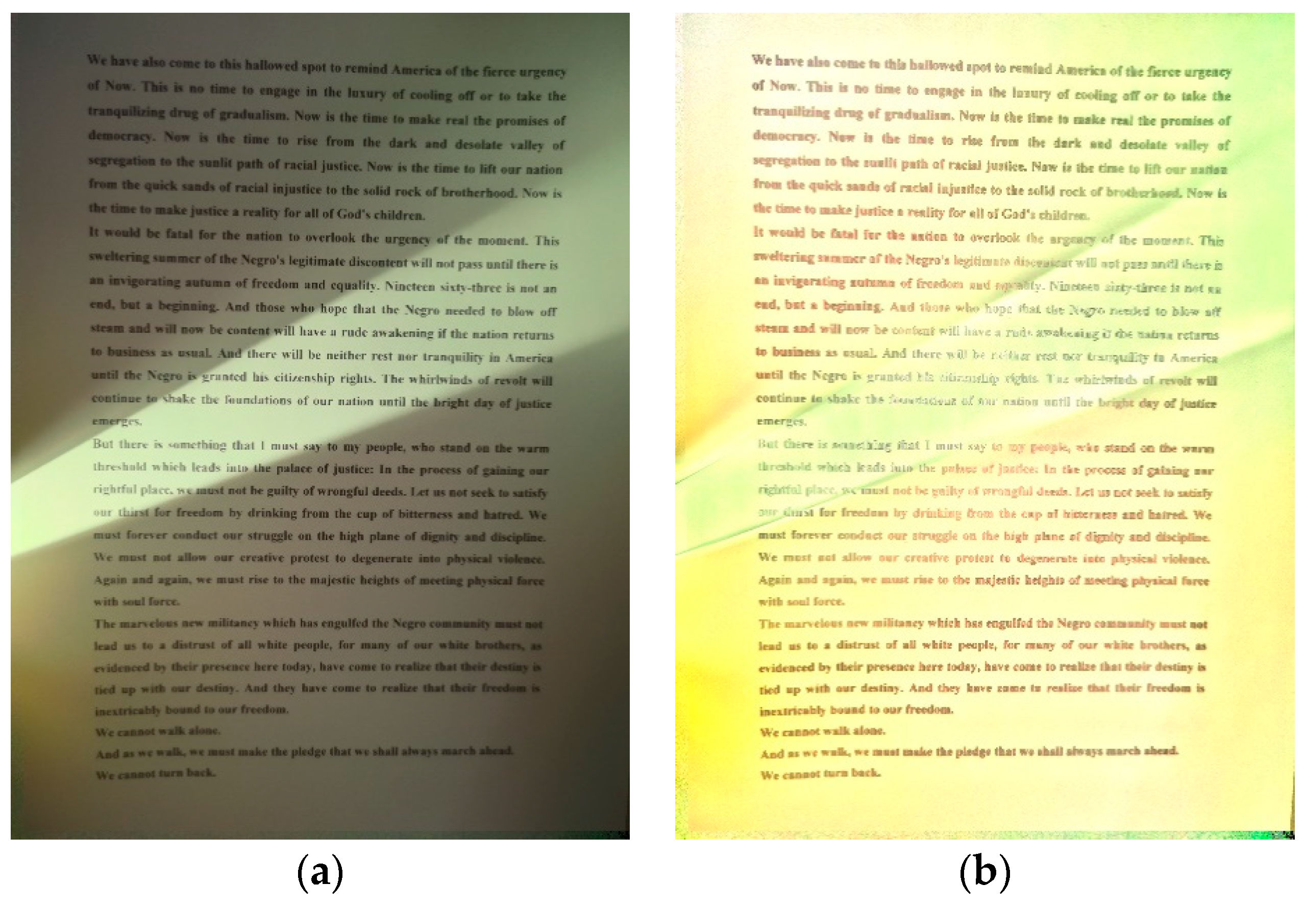
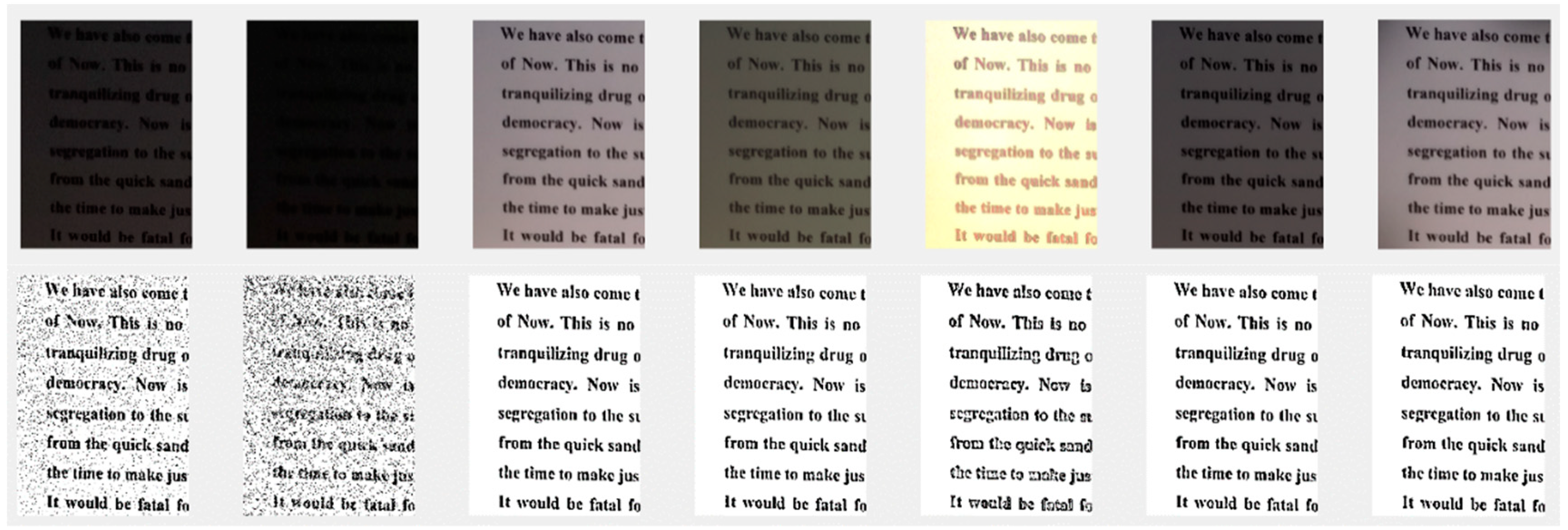
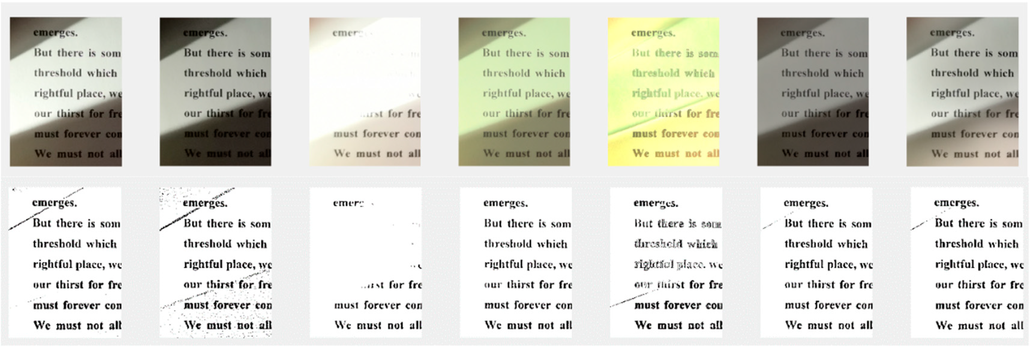
Figure 4 shows two pseudo color image patches that are composed of two LDR images that are already illustrated in Figure 1. The green band and blue band come from the corresponding bands in the well-exposed image while the red band is from the corresponding band in the over-exposed image. If there are no geometric disparities between these two images, the foreground (textual part) of the image should overlap. In Figure 4, we can clearly see that geometric difference exists as the foreground texts do not overlap. On top of it, we can clearly see that the global translational model cannot account for the geometric disparity between these two images. For example, Figure 4a is the left central image patch and we can see that the geometric difference between the well-exposed image and over-exposed image in this region is around 10 pixels (half the size of the lowercase letter “a”) in the vertical direction. However, in Figure 4b, the right central image patch, we can see that the geometric difference between the well-exposed image and over-exposed image in this region is around 20 pixels (the size of the lowercase letter “a”) in the vertical direction. This is obvious evidence that the geometric disparity between LDR images cannot be translational and that it must follow a more complicated geometric model.

Among all the geometric models, such as the affine model, translational model, rotation model, and so on, we ended up selecting the planar homograph model [6] to represent the geometric disparity between LDR images. Under this model, points in two different images can be mapped as:

$$\left(\begin{array}{c}{x}^{\prime }\\ y^{\prime }\\ z^{\prime }\end{array}\right)=\left[\begin{array}{ccc}a& b& c\\ d& e& f\\ g& h& 1\end{array}\right]\left(\begin{array}{c}x\\ y\\ z\end{array}\right)$$

(1)

where points are represented by homogeneous coordinates and so point (x, y, z) is the same as (x/z, y/z) in the inhomogeneous coordinate. We selected this model because during the bracketing stage, hand-shake is inevitably introduced, leading to different imaging angles for the same document object, and the planar homograph model is suitable for the situation where the imaging object is put on a planar surface and is captured from different view-angles.

When the planar homograph model is selected, we have to estimate this model’s eight parameters. Basically, there are two methods [7]. The first method is called the area-based method. Using this method to estimate the planar homograph model involves two steps: in the first step, a moving window is defined in the reference image and the image patch within the window is regarded as the template. We used the template to search for a corresponding image patch in the sensed image (an image that was registered). The centers of matched image templates are used as control points (CPs). There are many ways of finding a matching template, and one of the most popular criteria is cross correlation. When multiple CPs are generated, we then use these CPs to estimate the planar homograph model. Area-based methods, however, are not employed due to two reasons: (1) the first reason is that this method is computationally heavy as it performs cross correlation on multiple image patches and (2) the second reason is that image patches under different exposure levels may display extremely different characteristics, which may fail cross the correlation method.

The second method to estimate the planar homograph transformation is called the feature-based method. Two critical steps in feature-based methods are feature extraction and feature matching. We expect that the extracted features will be consistent regardless of exposure levels and among all the feature extraction methods, we selected the Scale-invariant Feature Transform (SIFT) method [8] because it improves detection stability in situations of illumination changes. In the meantime, it achieves almost real-time performance and the features that are detected are highly distinctive. SIFT does not only define the position of detected points, but also provides a description of the region around the feature point by means of a descriptor, which is then used to match SIFT feature points. Therefore, we have used the SIFT method to find CP pairs. 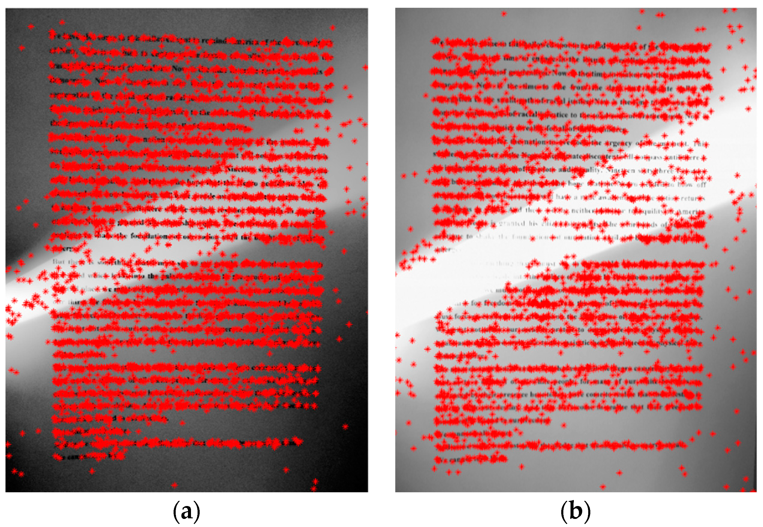Figure 5 shows the extracted matched SIFT features for two LDR images.

As we can observe from Figure 5, some SIFT feature points that cannot find correct corresponding pairs always exist. Therefore, some CP pairs cannot be used for inferring the planar homograph model as they are outliers. In order to remove these outliers, we used the Random Sample Consensus (RANSAC) algorithm combined with spatial constrains to prone the outliers [9]. The basic idea behind this is that we can estimate the planar homograph model with four randomly selected points. With the estimated model, we can check how close the CP pair is if they are put in the same coordinate system after transformation with formula (1). Then we calculate how many CP pairs are consistent with the estimated projective transform model, which indicates the confidence level of the estimated projective transform model. We performed this procedure multiple times and selected the projective model with the highest confidence level. After that, we re-estimated the projective model once again using the least-square method with all the CPs that fit the selected model. 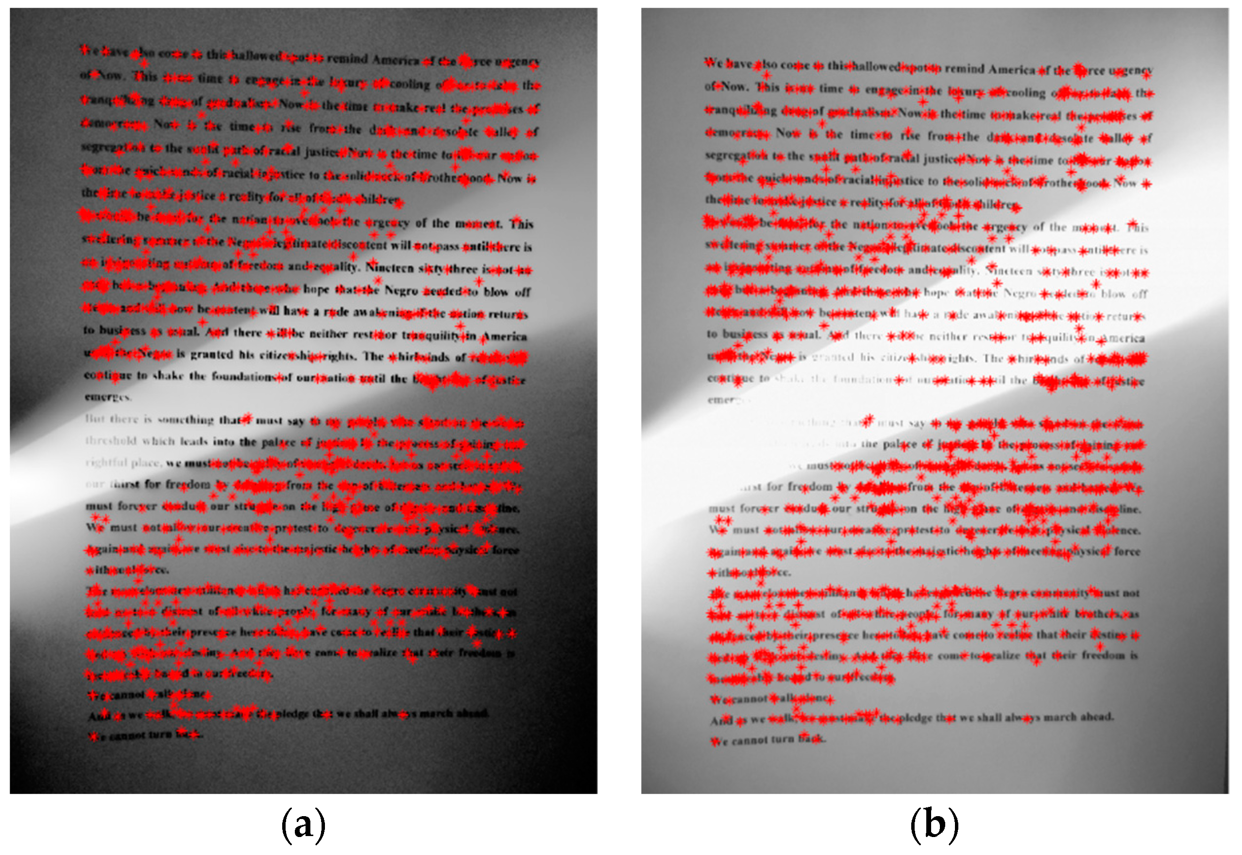Figure 6 shows the selected CPs that can be used to infer the planar homograph model using the above point pruning procedure. From this figure, we can clearly observe that all the outliers have been removed and each SIFT point in one image can always find its correct counterpart in another image.

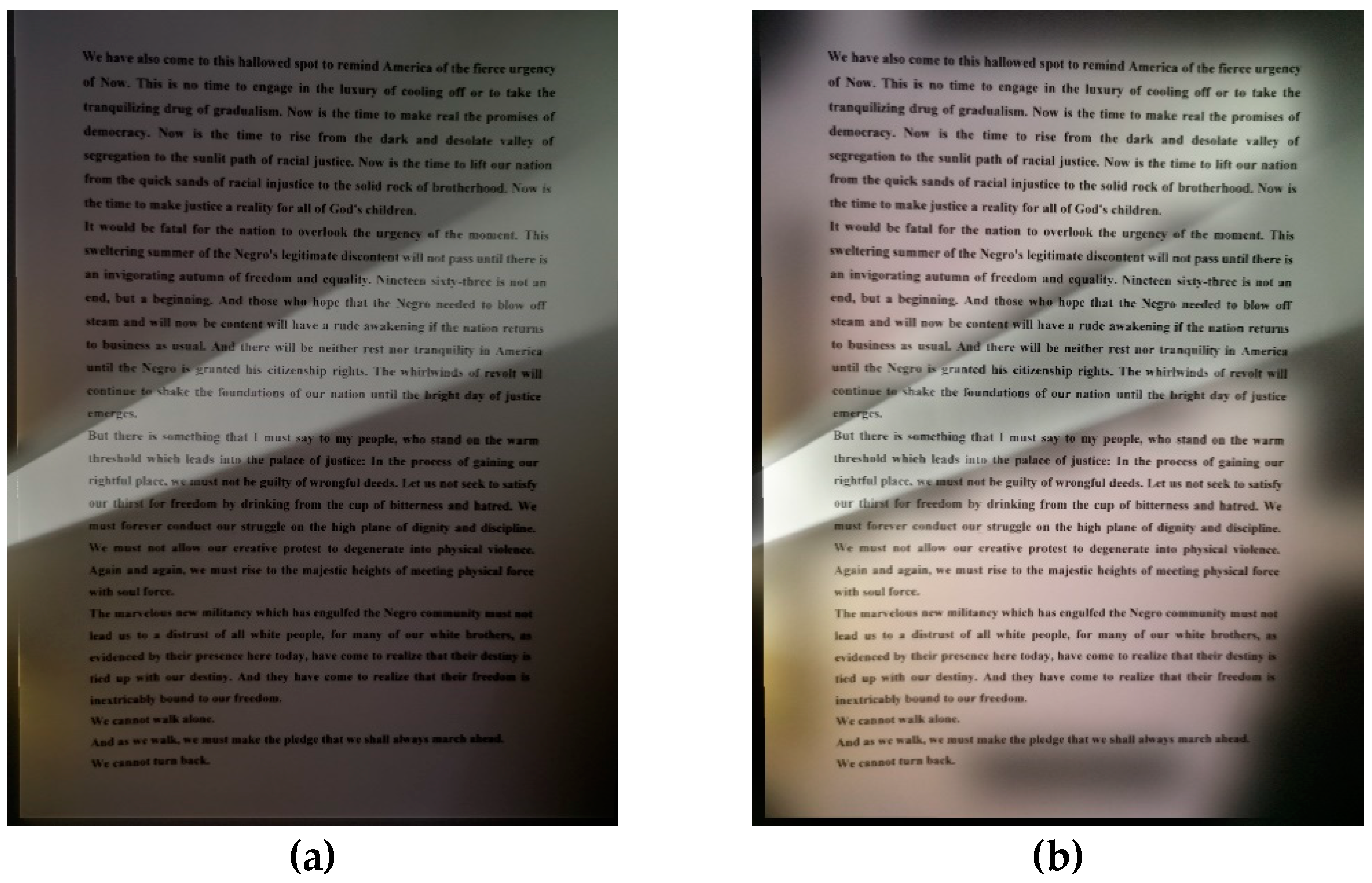
After the planar homograph model is estimated, we can perform the registration so that pixels from the same target share the same coordinate in the image stack. Figure 7 shows the pseudo color image after the registration, where the color configuration is the same as Figure 4. Overlapping the registered image of different exposure levels shows that a decent registration result has been obtained.

3.2. Tone Mapping Method

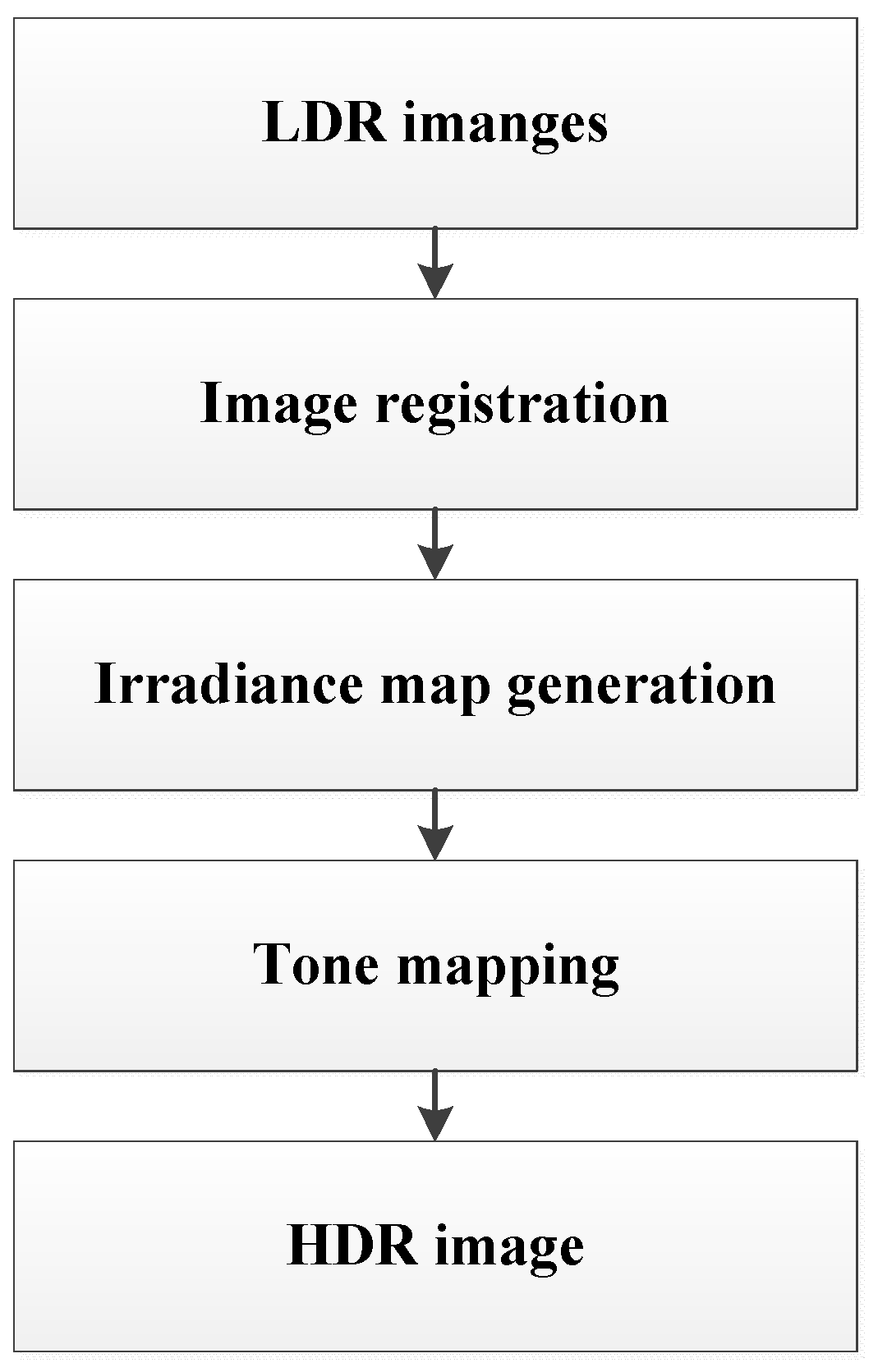
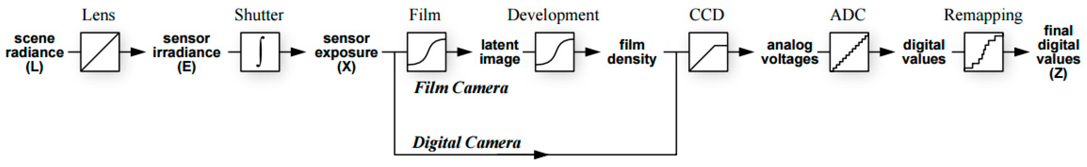
The tone mapping method can generate an HDR image by capturing multiple images of the same scene at different exposure levels and merging them to reconstruct the original dynamic range of the captured scene. In order to understand why HDR is possible with multiple images of different exposure times, it is necessary to know the image acquisition pipeline, which is illustrated in Figure 8.

Figure 8 shows how scene radiance becomes pixel values for both film and digital cameras, and we can use an unknown aggregate nonlinear mapping function to transform scene radiance L to digital pixel values Z. The unknown aggregate nonlinear mapping function is called the camera response function (CRF). It attempts to compress as much of the dynamic range of the real world as possible into the limited 8-bit storage. There are many methods that exist in the literature on how to estimate CRF and in this paper, we used the classical CRF estimation method that was proposed by Debevec and Malik [10]. With this method, estimating CRF is equal to optimizing the following objective function:

$$o={{\displaystyle \sum _{i=1}^{N_e}{\displaystyle \sum _{j=1}^M\left(\omega \left(I_i\left(x_j\right)\right)\left[g\left(I_i\left(x_j\right)\right)-\log E\left(x_j\right)-\log \Delta t_i\right]\right)}}}^2+\lambda {{\displaystyle \sum _{x=T_{\min }+1}^{T_{\max }-1}\left(\omega \left(x\right)g^{″}\left(x\right)\right)}}^2$$

(2)

where $g=f^{-1}$ is the inverse of the CRF, M is the number of pixels used in the minimization, $T_{\max }$ and $T_{\min }$ are, respectively, the maximum and minimum integer values in all LDR images $I_i$, $N_e$ is the number of LDR images, and $\omega$ is a weighting function defined as:

$$\omega \left(x\right)=\{\begin{array}{ll}x-T_{\min }& if x\le \frac{1}{2}\left(T_{\max }+T_{\min }\right)\\ T_{\max }-x& if x>\frac{1}{2}\left(T_{\max }+T_{\min }\right)\end{array}$$

(3)

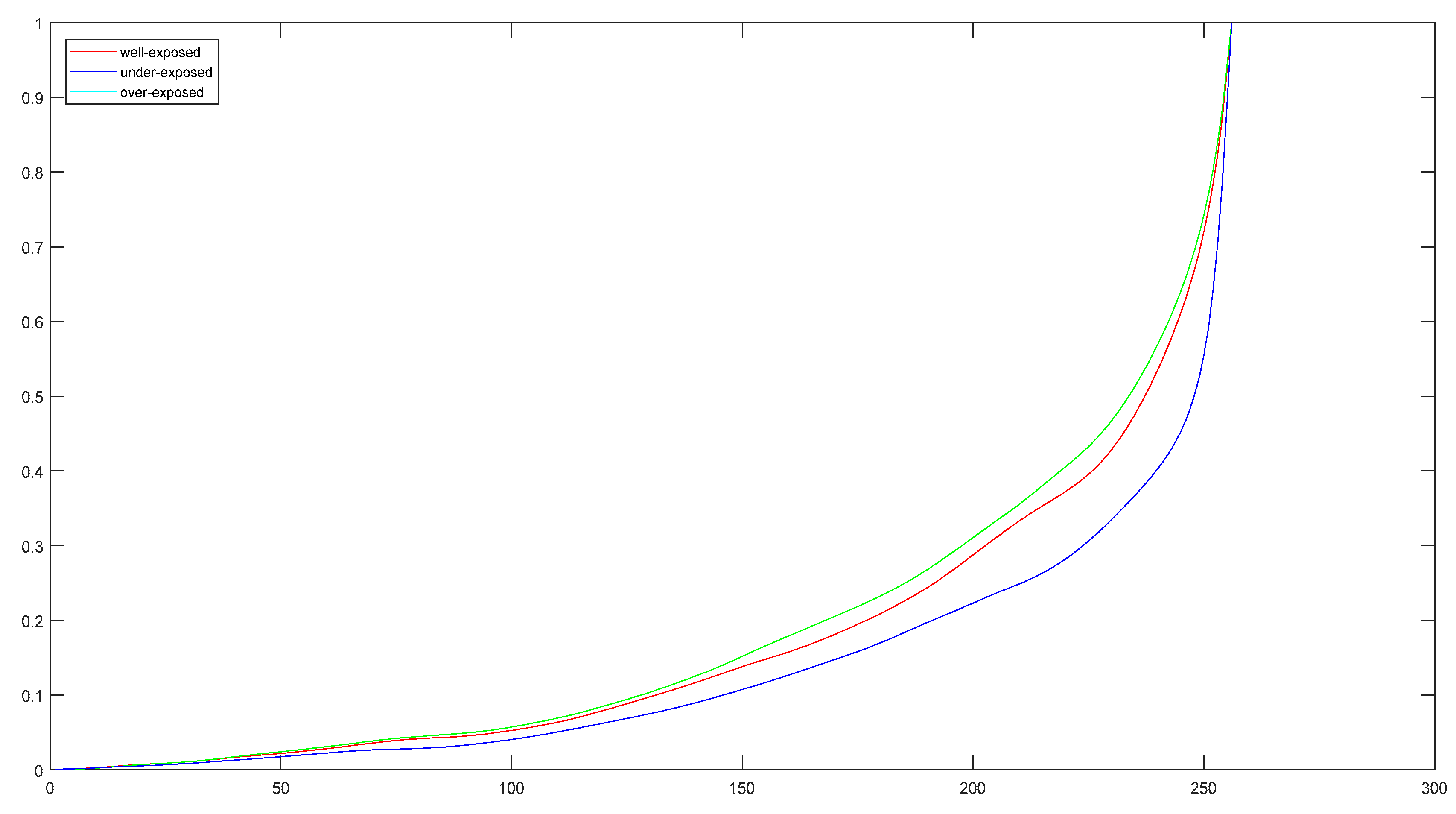
The implementation of Debevec and Malick’s method relies on the HDR Matlab Toolbox [3] and with this method, the estimated reverse CRF functions for images captured in Figure 1 are shown in Figure 9.

Once the reverse CRF is recovered, it can be used to quickly convert pixel values to relative radiance values based on the following formula:

$$\ln E_i=\frac{{\displaystyle \sum _{i=1}^P\omega \left(Z_{ij}\right)\left(g\left(Z_{ij}\right)-\ln \Delta t_j\right)}}{{\displaystyle \sum _{j=1}^P\omega \left(Z_{ij}\right)}}$$

(4)

The unit of radiance is of double-float format in order to keep the high dynamic range of real-world radiance, while most monitors can only display 255 colors. Therefore, in the last two decades, researchers have spent a significant amount of time and effort on compressing the range of HDR images and videos so that data may be visualized more naturally on LDR display.

Tone mapping is the operation that adapts the dynamic range of HDR content to suit the lower dynamic range that is available on a given display. Furthermore, only luminance is usually tone mapped by a tone mapping operator (TMO), while colors are unprocessed.

The TMO processing chain is as follows [11]:

Step 1: the luminance channel is first extracted from the radiance map and color information compression is avoided.

Step 2: the luminance is mapped to (0, 255) with a TMO.

Step 3: the following formula is used to obtain the mapping RGB channels:

$$\left[\begin{array}{l}{R}_d\\ G_d\\ B_d\end{array}\right]=L_d{\left(\frac{1}{L_w}\left[\begin{array}{c}{R}_w\\ G_w\\ B_w\end{array}\right]\right)}^s$$

(5)

where s is a saturation factor that decreases saturation. Tone mapping often increases saturation and hence, s is a floating value that is less than 1.

Step 4: Gamma correction is applied and each color channel is clamped in the range (0, 255).

TMOs are mainly composed of two methods:

(1) Global operators. With global operators, the same operator is applied to all pixels of the input image, preserving global contrast. They are non-linear functions based on the luminance and other global variables of the image. Once the optimal function has been estimated according to the particular image, every pixel in the image is mapped in the same way, independent of the value of the surrounding pixels in the image. These techniques are simple and fast, however they can cause a loss of contrast.

(2) Local operator. In this case, the parameters of the non-linear function change in each pixel, according to features extracted from the surrounding parameters. In other words, the effect of the algorithm changes in each pixel according to the local features of the image. These algorithms are more complicated than the global ones, they can show artifacts (e.g., halo effect and ringing), and the output can look unrealistic, however they can (if used correctly) provide the best performance since human vision is mainly sensitive to local contrast.

Among all the TMO operators provided by the HDR Matlab Toolkit, we selected one global TMO method, the ReinhardTMO method [12], and one local method, the DurandTMO method [13], for comparison.

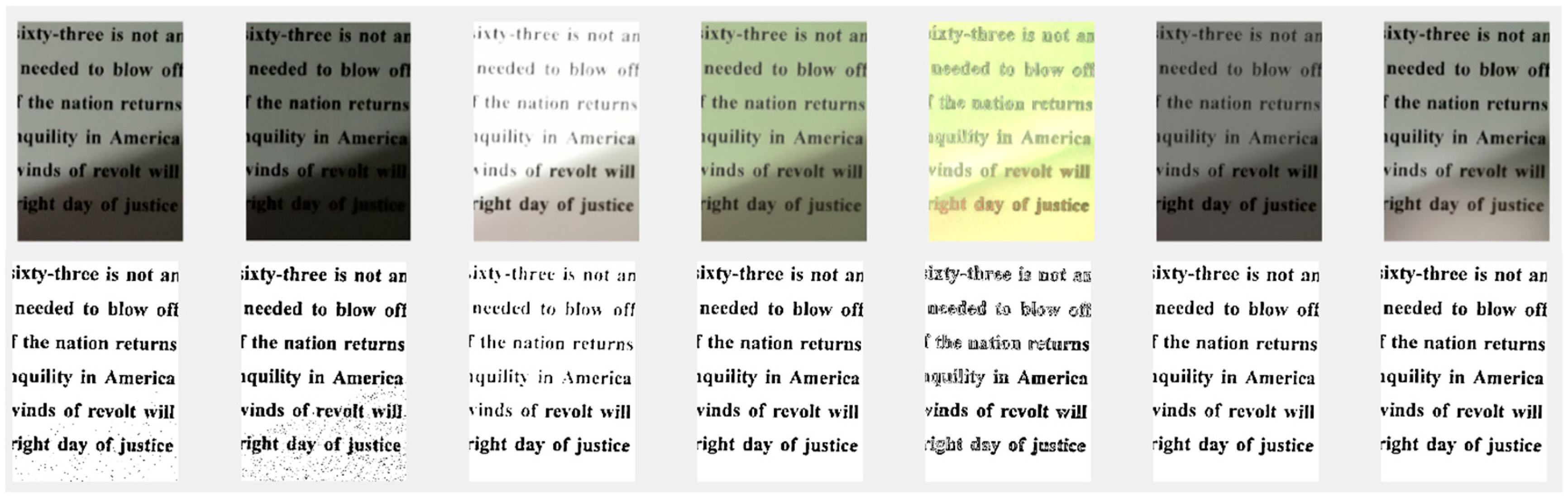
Figure 10 shows the ReinhardTMO method result and DurandTMO method result for the datasets that are shown in Figure 1. Visually, we can see some general improvements compared to the original captured images. However, the improvement may be negligible for some areas in the image. On top of it, we also observe that color distortion exists in the result images, and this becomes more obvious for the DurandTMO method.

3.3. Exposure Fusion

Exposure fusion merges differently exposed images using a weighted blending process. This approach has some advantages: it is less computationally expensive and there is no need to calibrate the camera response curve before transforming the pixel values to irradiances. The result is still a low dynamic range image, but it is overall better exposed and overall more aesthetically pleasant. In this paper, we selected two classical exposure fusion methods [14,15] to evaluate their document image enhancement performance.

3.3.1. Mertens’ Exposure Fusion Method

Mertens’ exposure method [14] was selected because this method has been incorporated in the latest OPENCV library, which indicates its influence. For any exposure fusion method, there are two questions to answer: the first is how to select good weights for each LDR image pixel and the second is how to blend the weighted pixels into the final result.

For the first problem, in Mertens’ exposure fusion method, three measures are used to select and weight the pixels: (a) Exposedness E(p): this measure is applied to each color channel separately, then the weights are multiplied. Considering that the pixel values range from 0 to 1, it preserves the pixels that are not too close to the boundaries. A Gaussian curve centered at 0.5 is suggested:

$$E\left(p\right)=\exp \left(-\frac{{\left(p-0.5\right)}^2}{2{\sigma }^2}\right)$$

(6)

(b) Contrast D(p): the contrast is closely related to details in local regions. A filter is applied on the grayscale version of the image to enhance details, and D(p) measures the absolute value of the filter response. The filter can be a 3 by 3 Laplacian filter. The basic idea is that over- or under-exposed parts of the image contain few details, while most of the details are in well-exposed regions. (c) Saturation S(p): the saturation is computed as a standard deviation from the R,G,B channels at each pixel. The reasoning behind this is that saturated colors look better in the well-exposed regions.

The final weight for each pixel in the LDR image is a combination of these three measures using multiplication. Finally, the weighting is normalized by making the sum of the weights equal to one. However, after the weights are calculated, simply linearly blending LDR images does not yield the desired result because the intensities vary wildly among the different images and may contain very sharp transitions. Therefore, a multi-resolution blending based on image pyramid decomposition is used. According to this scheme, a range of Laplacian pyramids are built for input LDR images and their corresponding weight maps are decomposed as Gaussian pyramids. For each pyramid level, regular blending is performed, generating a new Laplacian pyramid for the final result. Finally, the newly generated Laplacian pyramid is collapsed to obtain the output image.

3.3.2. Goshtasby’s Exposure Fusion Method

Goshtasby’s exposure fusion [15] is another widely employed fusion method. The basic idea behind this method is that we can use Entropy to select the best image patch among all LDR images as Entropy can be used to express the image patch’s quality. In order to remove discontinuities across image blocks, a blending function is proposed to assign the maximum weight to the pixel at the center of a block and assigns weights to other pixels that are inversely proportional to their distance to the center of block. The blending function that is employed is the rational Gaussian surface function:

$$W_{jk}(x,y)=\frac{G_{jk}\left(x,y\right)}{{\displaystyle {\sum }_{m=1}^{n_r}{\displaystyle {\sum }_{n=1}^{n_c}{G}_{mn}\left(x,y\right)}}}$$

(7)

where $n_r$ and $n_c$ denote the number of image blocks vertically and horizontally and $G_{mn}(x,y)$ represents the value of a Gaussian function centered at the jkth block. Two parameters must be set in this method: the first parameter is the image patch size and the second parameter is the standard deviation of the Gaussian function in (7). These parameters can be set empirically or can be searched in such a way that the output result reaches the best Entropy among all the parameter candidates. In our experiment, we set the parameters empirically as we found that parameter searching is too time-consuming because we would have to generate multiple intermediate output images. With the empirical setting, we divide the image into 20 by 20 images horizontally and vertically, and the Gaussian standard deviation is set to be equal to the square root of the image patch size.

As shown in Figure 11, we can see that the fusion method obtained good results. In order to clearly compare the output HDR image with the input LDR images, we zoomed in on some regions to visually see whether the HDR image enhanced the image quality or not, and we found that the texts in HDR are more vivid and the background is more homogeneous.

4. Experiments

In order to have a more objective evaluation of improved image quality due to exposure bracketing as well as a more objective comparison of different HDR generation methods, we used two methods for comparison. First, we zoomed in different regions of the well-exposed image, corresponding to a well-exposed region, under-exposed region, and over-exposed region of the image, and we then compared these regions with the HDR images and fusion images. In the meantime, we also generated the binary images of these regions using the Sauvola method. The reason why we also considered a binary image is because it is the binary image that will be used for OCR. Figure 12 shows one of the well-exposed regions in the well-exposed image. It is very clear that in this region, the original well-exposed image has good image quality and the moderate uneven lighting will not affect the generated binary image as the Sauvola binarization method is an adaptive image processing method. The same region in the under-exposed image shows small deterioration, however this is not observable in the well-exposed image. All HDR images and fusion methods show decent results. Figure 13 shows one of the under-exposed regions in the well-exposed image. This is the situation where we can clearly see the advantage of using exposure bracketing. The under-exposed image and well-exposed image do not have decent image quality, leading to noisy binary images. All the images generated with exposure bracketing techniques lead to improved image quality. Figure 14 shows one of the over-exposed regions in the well-exposed image. For this image patch, we can see that the over-exposed image, which has good binary output in Figure 12 and Figure 13, shows very bad results. Some textural information has been completely lost and the adaptive binarization method can no longer retrieve it. On the contrary, all the exposure bracketing methods can always retrieve good results regardless of the imaging conditions.

In order to further verify our visual observation, we began to use OCR accuracy as a criterion to justify the improved image quality due to exposure bracketing techniques. The philosophy behind this is that normally OCR accuracy is correlated with input image quality, and the better quality the document image has, the better OCR accuracy we can expect. Therefore, we set up a benchmark that was composed of 12 datasets for testing. The OCR toolkit we used is from open source Tesseract OCR [16], and the OCR accuracy was calculated based on open source ISRI Analytic Tools for OCR Evaluation [17]. The experiment results are shown in

Table 1. Optical Character Recognition (OCR) Accuracy.

	Well-Exposed	Under-Exposed	Over-Exposed	ReinhardTMO	DurandTMO	Goshtasby	Mertens
Error Character Number	920	2134	103	40	46	51	76
OCR Accuracy	58.50%	3.74%	95.35%	98.20%	97.93%	97.7%	96.57%

:

From Table 1, we can clearly see the value of exposure bracketing for increasing OCR accuracy, and the best OCR result with LDR images comes from over-exposed images with 103 error characters in total. All the exposure bracketing methods increased the original LDR image’s quality, leading to increased OCR accuracy.

5. Conclusions

In this paper, we investigated the potential of exposure bracketing techniques for improving the quality of camera document images. Four state-of-the-art algorithms were selected for investigation, their technical details were explained, and their intermediate results were illustrated. Positive experiment results show that using this technique can not only enhance the text readability, but can also lead to increased OCR accuracy.

In the meantime, we also proposed a processing chain that makes it possible to incorporate different bracketing algorithms. The feature-based registration method, relying on SIFT feature points and a robust RANSAC algorithm, and planar homograph geometric model have proved to be robust and effective when aligning multiple input images of different exposures.

References

1. Bukhari, S.S.; Shafait, F.; Breuel, T.M. Adaptive binarization of unconstrained hand-held camera-captured document images. J. Univers. Comput. Sci. 2009, 15, 3343–3363. [Google Scholar]
2. Sauvola, J.; Pietikainen, M. Adaptive document image binarization. Pattern Recognit. 2000, 33, 225–236. [Google Scholar] [CrossRef] [Green Version]
3. Banterle, F.; Artusi, A.; Debattista, K.; Chalmers, A. Advanced High Dynamic Range Imaging: Theory and Practice; Peters, A.K., Ed.; CRC Press: Natick, MA, USA, 2011. [Google Scholar]
4. Block, M.; Schaubert, M.; Wiesel, F.; Rojas, R. Multi-Exposure Document Fusion Based on Edge-Intensities. In Proceedings of the Theinternational Conference on Document Analysis and Recognition, Barcelona, Spain, 26–29 July 2009; pp. 136–140. [Google Scholar]
5. Luqman, M.M.; Gomez-Krämer, P.; Ogier, J.M. Mobile phone camera-based video scanning of paper documents. In International Workshop on Camera-Based Document Analysis and Recognition; Springer: Cham, Switzerland, 2013; pp. 164–178. [Google Scholar]
6. Klein, F. Elementary Mathematics from an Advanced Standpoint; Macmillan: New York, NY, USA, 1939. [Google Scholar]
7. Salvi, J.; Matabosch, C.; Fofi, D.; Forest, J. A Review of recent range image registration methods with accuracy evaluation. Image Vis. Comput. 2007, 25, 578–596. [Google Scholar] [CrossRef]
8. Lowe, D.G. Object recognition from local scale-invariant features. In Proceedings of the International Conference on Computer Vision, Kerkyra, Greece, 20–27 September 1999; pp. 1150–1157. [Google Scholar]
9. Kim, T.; Im, Y. Automatic satellite image registration by combination of stereo matching and random sample consensus. IEEE Trans. Geosci. Remote Sens. 2003, 41, 1111–1117. [Google Scholar]
10. Debevec, P.E.; MALIK, J. Recovering high dynamic range radiance maps from photographs. In SIGGRAPH 97 Conference Proceedings; Annual Conference Series; Wesley, A., Whitted, T., Eds.; ACM Siggraph: New York, NY, USA, 1997; pp. 369–378. [Google Scholar]
11. Devlin, K.; Chalmers, A.; Wilkie, A.; Purgathofer, W. Tone Reproduction and Physically Based Spectral Rendering. Eurographics 2002. Available online: https://www.researchgate.net/publication/2539412_Tone_Reproduction_and_Physically_Based_Spectral_Rendering (accessed on 23 October 2019).
12. Reinhard, E.; Stark, M.; Shirley, P.; Ferwerda, J. Photographic Tone Reproduction for Digital Images. ACM Trans. Graph. 2002, 21, 267–276. [Google Scholar] [CrossRef]
13. Durand, F.; Dorsey, J. Fast Bilateral Filtering for the Display of High-Dynamic-Range Images. ACM Trans. Graph. 2002, 21, 257–266. [Google Scholar] [CrossRef]
14. Mertens, T.; Kautz, J.; Van Reeth, F. Exposure Fusion: A Simple and Practical Alternative to High Dynamic Range Photography. Comput. Graph. Forum 2009, 28, 161–171. [Google Scholar] [CrossRef]
15. Goshtasby, A.A. Fusion of multi-exposure images. Image Vis. Comput. 2005, 23, 611–618. [Google Scholar] [CrossRef]
16. GitHub. Available online: https://github.com/tesseract-ocr/tesseract (accessed on 23 October 2019).
17. GitHub. Available online: https://github.com/Shreeshrii/ocr-evaluation-tools (accessed on 23 October 2019).
Figure 1. Camera document images with different exposure times. (a) exposure time: 1/800 s (under-exposed). (b) exposure time: 1/320 s (well-exposed). (c) exposure time: 1/40 s (over-exposed).
Applsci 09 04529 g001
Figure 2. Tone mapping processing chain.
Applsci 09 04529 g002
Figure 3. Exposure fusion processing chain.
Applsci 09 04529 g003
Figure 4. Pseudo color image composed of Figure 1a,c. The green and blue bands come from the green and blue bands of Figure 1b, while the red band is from the red band of Figure 1c. (a) The small image patch from the bottom-left part of the pseudo color image. (b) The small image patch from the bottom-right part of the pseudo color image.
Applsci 09 04529 g004
Figure 5. (a) Matched Scale-invariant Feature Transform (SIFT) feature points for a well-exposed image (Figure 1a); (b) Extracted SIFT feature points for an over-exposed image (Figure 1c).
Applsci 09 04529 g005
Figure 6. (a) Selected SIFT feature points for a well-exposed image (Figure 1a); (b) Selected SIFT feature points for an over-exposed image (Figure 1c).
Applsci 09 04529 g006
Figure 7. Pseudo color image composed of registered Figure 1a,c. The green and blue bands come from the green and blue bands of the registered well-exposed image while the red band is from the red band of the registered over-exposed image. (a) The small image patch from the left central part of the pseudo color image. (b) The small image patch from the right central part of the pseudo color image.
Applsci 09 04529 g007
Figure 8. Image acquisition pipeline.
Applsci 09 04529 g008
Figure 9. The reverse camera response function (CRF) for red, green, and blue bands for the Figure 1 dataset.
Applsci 09 04529 g009
Figure 10. (a) High dynamic range (HDR) tone mapping operators (TMOs) with the ReinhardTMO method; (b) HDR TMOs with the DurandTMO method.
Applsci 09 04529 g010
Figure 11. HDR fusion method: (a) Mertens’ method (b) Goshtashy’s method.
Applsci 09 04529 g011
Figure 12. One well-exposed region in well-exposed images. From left to right: well-exposed image, under-exposed image, over-exposed image, ReinhardTMO HDR image, DurandTMO HDR image, Goshtashy fusion, and the Merten fusion method. The images in the top row correspond to RGB images and the images in the bottom row correspond to binary images.
Applsci 09 04529 g012
Figure 13. One under-exposed region in well-exposed images. From left to right: well-exposed image, under-exposed image, over-exposed image, ReinhardTMO HDR image, DurandTMO HDR image, Goshtashy fusion, and the Merten fusion method. The images in the top row correspond to RGB images and the images in the bottom row correspond to binary images.
Applsci 09 04529 g013
Figure 14. One over-exposed region in well-exposed images. From left to right: well-exposed image, under-exposed image, over-exposed image, ReinhardTMO HDR image, DurandTMO HDR image, Goshtashy fusion, and the Merten fusion method. The images in the top row correspond to RGB images and the images in the bottom row correspond to binary images.
Applsci 09 04529 g014