Article

The Influence of Loading Program on the Stimulated Callus Mineralization

Institute of Applied Mechanics, Cracow University of Technology, al. Jana Pawła II 37, 31-864 Cracow, Poland
*
Author to whom correspondence should be addressed.
Appl. Sci. 2019, 9(20), 4268; https://doi.org/10.3390/app9204268
Submission received: 20 September 2019 / Revised: 2 October 2019 / Accepted: 4 October 2019 / Published: 11 October 2019
(This article belongs to the Section Applied Biosciences and Bioengineering)

Abstract

:
The aim of this work is to describe the change of physical properties of the callus material with the use of the proposed mathematical model for callus remodeling. Callus tissue can be considered as a biomaterial where it’s properties change over time due to the stimulated healing process. The proposed model is based on the mechanical stimulus theory. It is used to estimate the stress-stimulated change in the callus, Young’s modulus, and the density in the case of a mandible fracture. Three healing loading programs are discussed and compared: optimal, intermittent, and intermittent with residual load. Here, the optimal loading program is understood as the in-time change of stimulating loads, which results in the shortest necessary healing time and, simultaneously, in the most uniform distribution of material density in the analyzed domain. The necessary healing time is a period after which the callus density (and hence the Young’s modulus) reaches the desired value. The results of the study suggest a significant difference in the value of the callus maximal density between all three analyzed loading programs for a given healing time interval. The highest values of the density are obtained using the optimal loading program, however, all three programs provide satisfactory density distributions. The analytical results are compared with the callus density estimation based on the computer tomography (CT) medical data.

1. Introduction

The mandible (lower jaw) is the only load-bearing, moveable bone in the skull. Fractures in the mandible may happen as a result of infection, car accident, falling, sudden hit, or after a resection for pathology, e.g., cancer, treatment. As the only moveable bone of the cranium (skull), the mandible is subject to stresses and because of its shape, location, and function, the loads are unique to it [1]. This work focuses on the mandible fractures and healing process of the callus tissue after trauma. Such processes are known and thoroughly described for long bones, but in literature, there are no such works about mandible where complex states of stress and strain occur. The callus is a tissue formed between two bone parts after bone trauma. This process consists of three phases: reactive, reparative, and the remodeling phase during which different cells take part. In the first hours after the trauma, fibroblasts replicate and form a loose aggregate of cells, known as granulation tissue. Then, the fibroblasts within the granulation tissue develop into chondroblasts and this process culminates in a new mass of heterogeneous tissue, which is known as a fracture callus. The mineralized matrix is penetrated by osteoblasts, which form new lamellar bone in the form of the trabecular bone [2]. During the healing process, the properties of the callus tissue change make it mechanically stronger. The Young’s (elasticity) modulus of the callus, which increases in this process of mineralization, is used as an indicator of material mechanical properties. The soft callus tissue transforms into bone tissue [2]. There is a need for the formulation of mechanical models for biomaterial transformation, which enables computational analysis, eventually reducing animal studies or clinical trials, and helps to plan healing processes.
There are many ways to reconstruct the mandible. The most popular one involves plates and screws. It is noted that after the bone trauma the biomechanics of mandible changes [3]. It is not possible to load it with physiological values of the biting forces since they must be significantly reduced. During the first days after surgery, the patient may only eat slurry food using a straw. The most serious cases include very radical means when the braces and rails are used to immobilize the broken region of the mandible. In such cases, there are almost no stresses in the callus and, therefore, the tissue is not stimulated. It is noted that eating tough food too soon may lead to tissue resorption and it is important to keep the patient’s mandible immobilized [4,5]. Also, when micro-cracks occur under high tissue loading, bone resorption is induced [6,7].
According to Wolff’s law [8], tissue is able to change its internal material properties (i.e., density, Young’s modulus) to adjust to external loads placed upon it. This biological process is called remodeling. During this process, regulated by bone cells (osteoblasts and osteoclasts), both bone loss (resorption) and formation (apposition) may occur. Based on the Frost [9] mechanostat theory, bone tissue resorbs when the stimulus value drops below a certain threshold value, but formation occurs when the stimulus exceeds the upper threshold value. If a value of the mechanical stimulus remains in a lazy zone, i.e., between the lower and the upper values, remodeling does not take place. Since the applied load results in a specific strain-stress condition in the tissue material, it is accepted that the mineralization process is mechanically stimulated. It is observed that the speed of the mineralization process is not constant and changes continuously with the stimulus value. For a stimulus value beyond the lazy zone, the speed increases, reaches its maximum, and then decreases down to negative values; this is what denotes overload resorption process [3,10,11,12]. Indeed, overload resorption occurs when the mechanical stimulus increases too excessively. This theory for bone remodeling is adjusted and used as a new approach to describe the change in the callus density because during the mineralization process, the properties of the material (callus) change as an effect of external loading.
The mechanical stimulus theory states that there are some quantities, that can be calculated, which elicit or accelerate a physiological activity or response of the tissue. In this work, we focus on the physiological response of the callus tissue to external load action, exhibited in the corresponding change of its density. There are many factors considered as the mechanical stimuli: strain, stress, and deformation energy [13]. The mechanical stimulus theory for bone remodeling was proposed by Weinans et al. [14]. This theory states that the strain energy density (SED) is the most favorable factor that induces bone growth. The remodeling theory includes mass density, remodeling constants, reference values of the stimulus and a percentage value denoting the width of the lazy zone region [13]. One may notice that the mathematical description is divided into three parts. In the first one the negative change of bone density indicates bone resorption due to under-load, i.e., the stimulus is too small to induce bone growth. The second part describes the lazy zone where no growth and no loss occur. And the third part with the positive growth ratio, indicates bone growth and, therefore, tissue density increase. This most commonly used approach takes into account 3 stages: underload resorption, equilibrium, and bone growth (apposition) [13,15,16,17]. It is not the only possible formulation. Lin [10] proposed the mathematical description of overload resorption but it results in the function’s discontinuity, which can hardly be supported experimentally or clinically. This approach was later adopted by other authors [3,11] and mainly used to describe and predict the density of the bone tissue around the dental implants. Li [12] proposed the quadratic equation for the continuous description of bone remodeling but entirely omitted the lazy zone (equilibrium state). The “lazy zone” effect, initially proposed by Carter et al. in 1977 [18] based on experimental investigation, was verified by Rubin et al. [19] to be a relevant factor of the bone remodeling process, which should be included in the simulation. Some authors claim, based on the experimental study, that the idea of the “lazy zone” is controversial and they state that it is not valid [20]. However, in their study, Christen et al. included only a narrow group of post-menopausal women, thus the results might be questionable.
To sum up, only a few models proposed in the literature take into account bone resorption due to overload [3,10,12] and there are no such studies in relation to the callus material, which in the process of mineralization transforms into a compact bone tissue. Due to these facts, the aim of this work is to provide a new approach based on the mechanical stimulus theory to describe the change of the callus density in the process of healing. With the use of a mathematical model for callus remodeling [21,22], the analyses of various loading programs are performed. In this work, we mainly focus on the elastic modulus, E , of the callus tissue, i.e., we aim at obtaining its sufficiently high value and homogeneous distribution.
For the initial model validation, the medical data of the fractured mandible is analyzed. Firstly, the callus region based on the computer tomography data using Mimics software is marked, then the density measurements are performed. The aim of this analysis is to determine whether it is possible to determine the modulus of elasticity of the callus and compare its distribution qualitatively with the numerical analysis results.

2. Material and Methods

2.1. Geometry of the Callus Tissue

The proposed callus remodeling model [21,22] describes density change based on the mechanical stimulus theory using strain energy density (SED) in the stimulus definition. It should be clarified that the proposed model of tissue remodeling is used to analyze density changes only in the narrow section of the broken mandible in the process of stimulated healing and not in the mandible bone tissue. This section is a thin layer of the callus tissue of a shape similar to a rectangle and of 0.1–1.0 mm thickness (Figure 1), possibly stimulated during healing time. The section is subjected to loading as an effect of biting and muscular forces action. The result of load reduction to its centroid are mainly bending moment and shear force. In order to investigate the complex (not uniaxial) state of stresses and strains, a rectangular cross-section ( b × h ) loaded with bending moment and transverse force is considered. The initial value of the Young’s modulus ( E 0 ) is set to 2 MPa [23] and its initially uniform distribution is assumed all over the section. Due to non-uniform distribution of the stimulus, non-uniform healing is observed. The Young’s modulus which indicates that a bone may be loaded physiologically is set to 200 MPa after Knets [24]. Various loading programs may be considered for in-time change of the bending moment and shear force. The goal is to propose such a program that results in the fastest mineralization during mandible healing.
In the literature, a bone is considered to be an orthotropic or anisotropic material. However, in most finite element simulations, bone material (cortical tissue) is assumed to exhibit isotropic behavior [15,17,25,26,27,28,29,30,31]. There are mainly three reasons for that. Firstly, the relations between Young’s modulus and bone mass density are established experimentally mainly based on assumptions of material isotropy. Secondly, due to complex bone internal architecture, it is difficult to determine the orientation of the material properties in a bone. Thirdly, Milewski [32] conducted a finite element comparative analysis for the mandible with two different material properties (i.e., isotropic and orthotropic) and only a small difference was found between the results. From the biological point of view, in the process of mineralization, the callus tissue differentiates into mature bone tissue that exhibits the features of the cortical bone [2,33,34]. For these reasons, the isotropic material behavior for callus tissue is assumed in our analyses. It is worth mentioning that there are known various relations between tissue density and its Young’s modulus [13,35,36,37,38]. Some mathematical relations between the bone mass density and the mechanical properties (Young’s modulus) of the bone were experimentally established by other authors [25,31,37]. In this work, the elasticity modulus E (MPa) of the callus tissue is related to tissue mass density ρ (g/cm3):
E = C · ρ γ
where C and γ are the constants to be experimentally determined [39,40,41]. In this study C = 3790 MPa·cm9/g3 and γ = 3 are accepted following [13,14]. The callus tissue is modeled as a linear, elastic, and isotropic material for which constitutive relation is described with the use of two constants (the Young’s modulus, E , and the Poisson ratio, ν ).
According to Frost’s theory [9], a bone can adapt its internal architecture of the trabeculae together with its mechanical properties with regard to various mechanical stimuli. The strain energy density (SED) is widely used by other authors to predict and evaluate the remodeling process [3,10,11,13,20]. Moreover, the SED is very convenient to use because of its scalar character. In the proposed model, the local (point-level) callus density change is a function of the chosen mechanical stimulus, following the equation of remodeling rate [21]:
B ψ K min , 0 , D ψ K over 2 + K w , ψ < K min K min ψ K max ψ > K max
where ρ is the bone mass density (g/cm3), ψ denotes S E D / ρ (J/g), B and D are remodeling constants, K min , K max , and K over are the remodeling threshold values (J/g) and t (time unit) is the time parameter. K w is the maximal rate of density change (g/(cm3·time unit)) calculated as the top of parabola (Equation (2) row (3)) for ψ = K over .
The ordinary differential equation (Equation (2)) is solved numerically using the forward Euler method:
ρ t + Δ t = ρ t + d ρ d t · Δ t
Table 1 sums up the parameters used in the numerical analyses of bone remodeling in the mandible. It is worth pointing out that such parameters as K = K min + K max 2 , the effect of lazy zone, and the time constant regulating the remodeling rate are quite different in the literature.
The following values are used in this work for the model parameters: B = 1 ((g/cm3)2/(MPa·time unit)), D = K w K over K max K over K d = 31.847 [(g/cm3)3 (MPa·time unit)−1], K d = 0 , 0672   J / g , stands for the end of interval with positive remodeling rate ( ψ K max , K d ), K min = 0.0036 (J/g), K max = 0.0044 (J/g), K over = 0.0358 (J/g), δ = 10 % , K w = 0.0314 (g/(cm3·time unit)). In our simulation, at each time step, the change in callus density is calculated using Equation (2) at every material point of the rectangular section. Then, the corresponding Young’s modulus of the bone tissue is locally updated according to the Equation (1) and the analysis is carried out using the new, modified material properties. The iterative process continues until an acceptable distribution of the callus elasticity modulus is reached.

2.2. Analytical Formulation

As stated above, the rectangle is used to model the callus section of a broken mandible (Figure 1). The rectangle is loaded with the bending moment (couple) M together with the shear (transversal) force T . This results in non-homogeneous stress distribution over the section surface. Namely, they vary along the section height (coordinate z h / 2 , h / 2 ). Normal stress is expressed as:
σ z = M · E z · z I E   ,   I E = b h 2 h 2 E z · z 2 d z  
where IE (mm4∙MPa) denotes the weighted (generalized) moment of inertia, and the shear stress is:
τ z = T · S E z I E · b   ,   S E z = b h 2 z E ξ · ξ d ξ
where S E (mm3∙MPa) denotes the weighted static moment about a neutral axis of section cut-off lying on one side of level z .
Hence, the stimulus becomes a function of z , as do the Young’s modulus, E , and density, ρ . A complex stress state implies that the value of the strain energy density, S E D , varies along the height of the section:
S E D z = 1 2 E z σ z 2 + 1 + ν E z τ z 2

2.3. Optimal Loading Program

The previous studies [21,22], showed that for a constant-in-time load value, it is impossible to obtain a sufficiently high Young’s modulus even after an infinitely long time of healing. The question arises of how to choose a loading program (understood as functions in time for M t and T t ) so as to obtain the desired distribution of E z . In order to compare various distributions of the callus Young’s modulus over the healing domain (rectangle), as well as to assess sufficiency and homogeneity of a particular distribution, three parameters are defined and calculated: maximal value ( E max ), mean value ( E m ), and deviation parameter ( s )
s = h 2 h 2 E z E m 1 2 d z h
The less is s , the less is difference E max E m , the better (the more homogeneous) is the obtained distribution of E z . For the most desired uniform distribution, E z = const z , the deviation parameter s = 0 . The closer E max is to 200 (MPa), the more sufficient the distribution is. Hence, the optimal loading program is defined as either functions of M t and T t , which minimize s ( s m i n ) and maximize E max ( E max m a x ) in a given time interval, or equivalently, such functions of M t and T t , which minimize s ( s m i n ) and minimize the time necessary to obtain a desired value of E m a x (e.g., E max = 200 (MPa)).

3. Results

The results are presented in Figure 2, Figure 3 and Figure 4 for three analyzed loading programs. On the right side, each of ten colored lines represent the Young’s modulus distribution along the height of the analyzed rectangular section (Figure 1C) for the given time step ( t = 1 , 2 , 3 , , 10 ) . The first line on the left represents the starting point ( t = 0 ) with the initial value of the callus elasticity modulus equal to 2 MPa. Moving to the right, along the “time increase” arrow, we observe an increase of the Young’s modulus maximal value and the mean value in the callus. The three parameters of homogeneity are calculated for the final time step ( t = 10 (time unit)).
Figure 2 presents the outcome of a progressive remodeling process for the optimal loading program. The values of the bending moment, M , and shear force, T , in time, are calculated using the control algorithm described in [21,22]. This control algorithm is used for the load parameters so as to improve homogeneity of the elasticity modulus with possibly maximal remodeling rate. At each time step, we require that the value of the stimulus parameter ψ
ψ z = S E D z ρ z = c 3 2 · M 2 z 2 · E z 2 3 I E 2 + c 3 1 + ν E z 4 3 · T 2 S E z 2 I E 2 · b 2
is kept in a narrow vicinity of the optimal value, K over , for all section points, which denotes that the remodeling rate remains close to the maximal possible value, K w . Satisfying min z ψ z = 1 α K over and max z ψ z = 1 + α K over ( α determines the vicinity), we come to a set of equations to determine the optimal values of the bending moment, M , and the shear force, T . They are related to the distribution of E z obtained at the preceding time steps, starting from E z = const z = 2 (MPa) at time t = 0 .
c 3 2 · M 2 z min 2 · E z min 2 3 I E 2 + c 3 1 + ν E z min 4 3 · T 2 S E z min 2 I E 2 · b 2 = 1 α K over
c 3 2 · M 2 z max 2 · E z max 2 3 I E 2 + c 3 1 + ν E z max 4 3 · T 2 S E z max 2 I E 2 · b 2 = 1 + α K over
z max and z min denote coordinates of section points where the stimulus is maximal or minimal, respectively. With this optimal loading program it is possible to reach unrestricted value of the elasticity modulus with its distribution kept close to homogeneous. In Figure 2 (right plot), only the first 10 time steps are presented and the E max = 233 MPa, which fulfills the requirement of 200 MPa as an ending point of calculation. The left plots present the loading program as the time-variation of dimensionless bending moment and shear force. The dimensionless quantities are defined with the use of section dimensions ( b , h ) and the initial value of the callus Young’s modulus ( E 0 ).
M ˜ = M b · h 2 6 · E 0
T ˜ = T b · h · E 0
It is unlikely that in practical treatment of a patient, the load parameters ( M and T ) can be changed in continuous and optimal manner. The loading program might be interrupted and for a designated time interval, the loads may diminish to zero. The aim of investigating this intermittent loading program is to assess its influence on the final distribution of the callus elasticity modulus. The optimal load values ( M and T ) are applied for a given time interval ( Δ t load = 1   time   unit ) , hence the callus density (and elasticity modulus) increases due to Equation (2). Then the loads drop to zero for equal time intervals and the modulus decreases due to the resorption effect ( ψ < K min ) . The process is repeated that way for 10 time units. Figure 3 presents the outcome of the remodeling process for the intermittent loading program in which one may observe that, in general, a satisfactory homogeneous distribution of the Young’s modulus in a section is achieved ( s = 0.019 ). However, the maximal value of the elasticity modulus is almost five times lower than the value obtained for the optimal loading program after the same healing time (Table 2). This loading program can still provide a sufficient value for the elasticity modulus of the callus tissue but a longer time period is required (Table 3). The homogeneity of the “long time” distribution is worse than the one obtained for the continuous optimal loading program. Also, remodeling effectiveness depends on the ratio between loading ( Δ t load ) and unloading Δ t unload time intervals, and the bigger the ratio is, the higher the value of E max can be remodeled in the given time. This loading program was analyzed as physiological-like when during the healing process, the callus tissue is repeatedly stimulated and not stimulated for given time intervals.
Figure 4 presents the outcome of a progressive remodeling process for the intermittent loading program with the 10% residual load. That means the load values are assumed to reduce down to 10% of ones acting before unloading, instead of total vanishing. This program was analyzed only as a possibility to happen and the 10%, 20%, or 30% values for the residual loads are chosen to test how the model of the callus remodeling would respond to this type of loading scheme. Comparison of the load paths in Figure 2, Figure 3 and Figure 4 indicates significantly different values. It is explained that optimal load values, calculated with Equations (9) and (10), are not established once for good. In contrary, they strongly depend on healing process history, exhibited by the modulus distribution E z , obtained after all the preceding time steps. If there is no unloading, as in the optimal program, the modulus increases continuously in time at all section points, and hence the required values of optimal M and T increase too. For the sub-optimal intermittent programs, the modulus increases during loading but decreases during each unloading period. In general, if a following loading is to start after an unloading time, the optimal values of loads are less because of smaller values of E z .
One may observe for the intermittent programs that for a given time interval (Table 2) the higher is the residual load the better are values of E max , but the distribution homogeneity is worse. Similarly, Table 3 indicates that for the intermittent programs the higher is the residual load the shorter is healing time, necessary for satisfactory E max value. However, the distribution homogeneity is worse. The explanation is, that during total unloading the resorption occurs with the same rate ( B K min (g/(cm3·time unit)) at each section point, since the stimulator ψ = 0 for each coordinate z . That means, the modulus is reduced for the same value everywhere and the distribution homogeneity is not changed after unloading. For partial unloading (intermittent with residuum), it happens that the modulus decreases in some section regions (where ψ < K min ), or remains unchanged in some regions (where K min < ψ < K max ), or increases elsewhere (where ψ > K max ). The last possibility is more likely to happen for higher residual loads. This results in the deterioration of the distribution homogeneity which is improved after the loading period.

4. Callus Density Measurements

The clinical studies of computer tomography data are strictly limited and mostly difficult to obtain. The patient’s medical scans are performed during clinical appointments, which are rarely regular as mostly they take place with unevenly spaced time intervals. Therefore, it is difficult to collect the supportive clinical data for model validation, especially for estimating its time-scale parameters. The idea is to compare a series of scans and hence, knowing the true healing time, to scale the model and establish the true time unit. Thus, in this research, the data set includes only two CT scans of a fractured mandible. The first CT scan was obtained a day after bone trauma, the second one 18 days after. In this study, we focus on determining the callus Young’s modulus based on the CT scans using Mimics software (V20.0, Materialise Co. Ltd., Leuven, Belgium). For this reason, we have excluded the first set of CT scans as there are no visible signs of the callus and the broken bone parts are evidently separated (
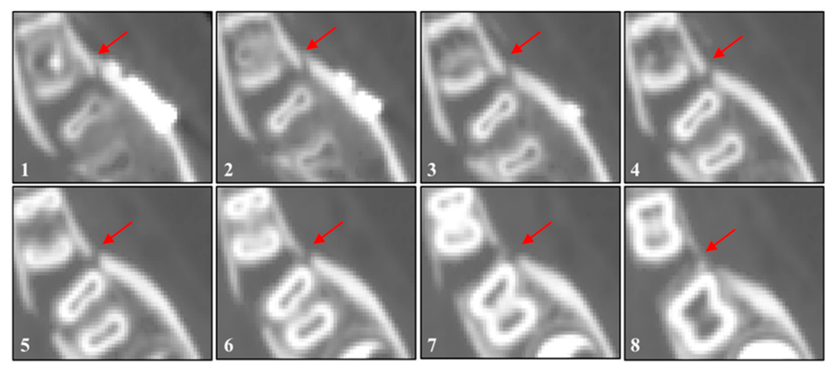
Figure 5). For the second set of CT scans, eight planes perpendicular to the forming callus tissue are chosen for analyses. They are shown in Figure 6 where the callus area for the density measurements is marked as a region between bone parts (red arrows) and shown as planes from the molar area to the area beside the fixing plate. Then, the measurements of radiological density units HU (Hounsfield scale) are performed around the formed callus tissue at every plane in the region between the bone parts. One may observe a sudden drop of the radiological density indicating the formed callus tissue, which is significantly lower than the one for the mandible bone parts. The tissue mass density is calculated by the software’s built-in equations. Then, using Equation (1), Young’s modulus of the callus tissue is calculated at every investigated point. The Young’s modulus distribution of the callus tissue along profile lines is presented in Figure 7. One may observe a sudden drop of the Young’s modulus along the profile lines indicating the formed callus tissue, where the modulus of elasticity is significantly lower than the one for the mandible bone parts. The minimum value for every profile line is chosen for further analysis. It is assumed that the minimum value indicates the region of forming of the callus tissue and represents its properties. The results of the Young’s modulus calculations for every plane are shown in Figure 7. The highest values of the elasticity modulus are observed for the planes at the upper part of the mandible, near the molar. The callus tissue Young’s modulus decreases in the direction from the molar to the fixing plate (Figure 5b blue part). The observed distribution of the modulus remains in good agreement with the calculated results in the qualitative sense. It indicates that the highest value is met at the top of the callus layer which is stimulated the most because of the highest value of normal stress.
It is not possible to compare directly or verify the results of the numerical or analytical analyses mainly due to the different loading program during patient’s rehabilitation. The exact values of the loads and forces are quite impossible to establish post-healing. Therefore the goal of this part of the work is to present a way to mark the callus region based on the CT data using Mimics software. As presented, it is possible to determine the modulus of elasticity based on the radiological density and compare its distribution qualitatively with the numerical analyses results.
For more adequate results, it seems necessary to obtain medical data from a patient at subsequent time intervals during the healing process. Unfortunately, CT scans are rarely performed in a short time space because of the fear for the patient’s health. Due to the X-rays used in that study, there is a risk of osteoradionecrosis (cell death due to radiation). The presented correlation between clinical data and numerical results are satisfactory at this moment of analyses but need further investigation with the full 3D model of the mandible.

5. Discussion

In our study the computational callus remodeling model is used to estimate how the loading program effects the callus density distribution during the stimulated healing process. Also, an attempt to establish the optimal loading program was made, leading to the most homogeneous distribution of material properties with nominal values kept on a desired level. Two sub-optimal approaches are studied in order to get closer to possible clinical treatment. Based on the numerical results, the callus remodeling response can be evaluated. The results of this study suggest a significant difference in the callus maximal density value between all three analyzed loading programs performed in the same time interval. The highest values of the density is obtained using the optimally-controlled model. All three programs provide satisfactory density distribution, although the intermittent programs require more time to achieve the designated 200 MPa Young’s modulus value.
There are three assumptions that have to be considered as limitations to accurately predict the outcomes of the callus distribution. First, the callus remodeling algorithm used in this work does not include the individual differences of the tissue density due to sex, age, diseases, osteoporosis, pharmacology treatment, and other patient-specific factors. Therefore, the influence of these factors on the callus remodeling process should be considered in the future study. That could mainly be achieved by variation of the model constant parameters. Due to that fact, the results presented and discussed here must be taken qualitatively and quantitative data will be different for each particular patient case. Second, the starting point of the iterative analysis is a homogeneous distribution of tissue density with Young’s modulus equal to 2 MPa. In fact, the callus density in the first day of the healing process was not fully investigated or thoroughly described [23,42,43,44]. Third, isotropic material properties were considered instead of anisotropic, which are closer to the true material. However, as mentioned before, in the process of mineralization, the callus tissue acquires the features of a cortical bone, which in the literature is mainly modeled as an isotropic material. Moreover, the very small thickness of the callus layer justifies this simplification.
One may observe from the above results that the proposed loading programs have a big influence on the bone density distribution. The predicted outcomes are not far different to those experienced in reality. It is known that too big a load can cause substantial damage or irreversible fracture in the tissues which are not strong enough [45,46]. Therefore, to strengthen the callus tissue after trauma, the load must be applied at an adequate rate and of an adequate value dictated by the bone density at the particular point of healing time. Qualitative and quantitative comparison between results shows a sufficient degree of resemblance between the computational results and the clinical CT data. Also, numerical studies prove that efficient healing of the tissue may be obtained in the realistic load-controlled treatment (intermittent program).
Simulations of callus remodeling, validated and compared with clinical data, are proven as a helpful way to elucidate the mechanisms behind bone healing. The effect of callus remodeling and the influence of the loading program on the healing process are critical for the development of planning the rehabilitation process. It is expected that this analyses of callus remodeling can contribute to the development of new loading programs used during patient rehabilitation. In the future, a detailed 3D analysis will be performed so that more a complex model of the callus and the mandible can be considered and more thorough solutions can be reached. The outcome of this research demonstrates the importance of the computational biomechanics due to the limitations in obtaining clinical data and experimental results. It substantiates the understanding of callus remodeling and provide new insights into bone healing. Additionally, it extends the potential of computer simulations in the field of bone biomechanics and hopefully, eventually reduce animal studies and clinical trials. Thoroughly examined numerical model of the callus stimulated transformation can be implemented into a finite element analysis of realistic (in shape and loading scheme) bones with thin layers of callus after trauma.

Author Contributions

Conceptualization, methodology, software, validation J.M. and J.B.; Writing—original draft preparation, J.M.; Writing—review and editing, J.B.

Funding

This research received no external funding.

Conflicts of Interest

The authors declare no conflict of interest.

References

  1. Wong, C.W.; Loh, J.S.P.; Islam, I. The Role of Finite Element Analysis in Studying Potential Failure of Mandibular Reconstruction Methods. Perusal Finite Elem. Method 2016, 189–210. [Google Scholar]
  2. Affshana, M.; Priya, J. Healing Mechanism in Bone Fracture. J. Pharm. Sci. Res. 2015, 7, 441–442. [Google Scholar]
  3. Wang, C.; Fu, G.; Deng, F. Difference of natural teeth and implant-supported restoration: A comparison of bone remodeling simulations. J. Dent. Sci. 2015, 10, 190–200. [Google Scholar] [CrossRef] [Green Version]
  4. Kromka-Szydek, M.; Jedrusik-Pawłowska, M.; Milewski, G.; Lekston, Z.; Cieślik, T.; Drugacz, J. Numerical analysis of displacements of mandible bone parts using various elements for fixation of subcondylar fractures. Acta Bioeng. Biomech. 2010, 12, 11–18. [Google Scholar] [PubMed]
  5. Jedrusik-Pawłowska, M.; Kromka-Szydek, M.; Katra, M.; Niedzielska, I. Mandibular reconstruction—Biomechanical strength analysis (FEM) based on a retrospective clinical analysis of selected patients. Acta Bioeng. Biomech. 2013, 15, 23–31. [Google Scholar] [PubMed]
  6. Burr, D.B.; Martin, R.B.; Schaffler, M.B.; Radin, E.L. Bone remodeling in response to in vivo fatigue microdamage. J. Biomech. 1985, 18, 189–200. [Google Scholar] [CrossRef]
  7. Mori, S.; Burr, D.B. Increased intracortical remodeling following fatigue damage. Bone 1993, 14, 103–109. [Google Scholar] [CrossRef]
  8. Wolff, J. The Law of Bone Remodelling; Springer: Berlin, Germany, 1986. [Google Scholar]
  9. Frost, H.M. Bone’s Mechanostat: A 2003 Update. Anat. Rec.—Part. A Discov. Mol. Cell. Evol. Biol. 2003, 275, 1081–1101. [Google Scholar] [CrossRef]
  10. Lin, C.L.; Lin, Y.H.; Chang, S.H. Multi-factorial analysis of variables influencing the bone loss of an implant placed in the maxilla: Prediction using FEA and SED bone remodeling algorithm. J. Biomech. 2010, 43, 644–651. [Google Scholar] [CrossRef]
  11. Wang, C.; Li, Q.; McClean, C.; Fan, Y. Numerical simulation of dental bone remodeling induced by implant-supported fixed partial denture with or without cantilever extension. Int. J. Numer. Method. Biomed. Eng. 2013, 29, 1134–1147. [Google Scholar] [CrossRef]
  12. Li, J.; Li, H.; Shi, L.; Fok, A.S.L.; Ucer, C.; Devlin, H.; Horner, K.; Silikas, N. A mathematical model for simulating the bone remodeling process under mechanical stimulus. Dent. Mater. 2007, 23, 1073–1078. [Google Scholar] [CrossRef] [PubMed]
  13. Mellal, A.; Wiskott, H.W.A.; Botsis, J.; Scherrer, S.S.; Belser, U.C. Stimulating effect of implant loading on surrounding bone. Clin. Oral Implants Res. 2004, 15, 239–248. [Google Scholar] [CrossRef] [PubMed]
  14. Weinans, H.; Huiskes, R.; Grootenboer, H.J. The behavior of adaptive bone-remodeling simulation models. J. Biomech. 1992, 25, 1425–1441. [Google Scholar] [CrossRef] [Green Version]
  15. Lian, Z.; Guan, H.; Ivanovski, S.; Loo, Y.C.; Johnson, N.W.; Zhang, H. Effect of bone to implant contact percentage on bone remodelling surrounding a dental implant. Int. J. Oral Maxillofac. Surg. 2010, 39, 690–698. [Google Scholar] [CrossRef] [PubMed] [Green Version]
  16. Field, C.; Li, Q.; Li, W.; Thompson, M.; Swain, M. Prediction of mandibular bone remodelling induced by fixed partial dentures. J. Biomech. 2010, 43, 1771–1779. [Google Scholar] [CrossRef]
  17. Lin, D.; Li, Q.; Li, W.; Duckmanton, N.; Swain, M. Mandibular bone remodeling induced by dental implant. J. Biomech. 2010, 43, 287–293. [Google Scholar] [CrossRef] [PubMed]
  18. Carter, D.R.; Hayes, W.C. The compressive behavior of bone as a two-phase porous structure. J. Bone Jt. Surg.—Am. Vol. 1977, 59, 954–962. [Google Scholar] [CrossRef]
  19. Rubin, C.T.; Lanyon, L.E. Regulation of bone mass by mechanical strain magnitude. Calcif. Tissue Int. 1985, 37, 411–417. [Google Scholar] [CrossRef]
  20. Christen, P.; Ito, K.; Ellouz, R.; Boutroy, S.; Sornay-rendu, E.; Chapurlat, R.D.; Rietbergen, B. Van Bone remodelling in humans is load-drivenbut not lazy. Nat. Commun. 2014, 5, 1–5. [Google Scholar] [CrossRef]
  21. Miodowska, J.; Bielski, J.; Kromka-Szydek, M. A new model of bone remodelling. Eng. Trans. 2016, 64, 605–611. [Google Scholar]
  22. Miodowska, J.; Bielski, J.; Kromka-Szydek, M. Callus remodelling model. AIP Conf. Proc. 2018, 1922, 1–9. [Google Scholar]
  23. Isaksson, H.; Wilson, W.; van Donkelaar, C.C.; Huiskes, R.; Ito, K. Comparison of biophysical stimuli for mechano-regulation of tissue differentiation during fracture healing. J. Biomech. 2006, 39, 1507–1516. [Google Scholar] [CrossRef] [PubMed]
  24. Knets, I.; Viltins, V.; Cimdins, R.; Laizans, J. Biomechanical behaviour of system bone-callus-implant. In Proceedings of the 10th Conference of the European Society of Biomechanics, Leuven, Belgium, 28–31 August 1996; Vander Sloten, J., Ed.; Pub. The European Society of Biomechanics: Leuven, Belgium, 1996; p. 97. [Google Scholar]
  25. Chou, H.-Y.; Jagodnik, J.J.; Müftü, S. Predictions of bone remodeling around dental implant systems. J. Biomech. 2008, 41, 1365–1373. [Google Scholar] [CrossRef] [PubMed]
  26. Yoda, N.; Zheng, K.; Chen, J.; Liao, Z.; Koyama, S.; Peck, C.; Swain, M.; Sasaki, K.; Li, Q. Biomechanical analysis of bone remodeling following mandibular reconstruction using fibula free flap. Med. Eng. Phys. 2018, 56, 1–8. [Google Scholar] [CrossRef] [PubMed] [Green Version]
  27. Datarkar, A.; Tayal, S.; Thote, A.; Galie, M. An in-vitro evaluation of a novel design of miniplate for fixation of fracture segments in the transition zone of parasymphysis-body region of mandible using finite element analysis. J. Cranio-Maxillofac. Surg. 2019, 47, 99–105. [Google Scholar] [CrossRef]
  28. Khiabani, K.; Keyhan, S.O.; Razmdideh, R.; Chaleh Chaleh, Z.; Amirzade-Iranaq, M.H. Effect of different miniplate osteosynthesis in different mandibular angle fracture patterns on bite force: A 3D finite element analysis. J. Oral Maxillofac. Surgery Med. Pathol. 2018, 30, 324–329. [Google Scholar] [CrossRef]
  29. Ribeiro, F.O.; Folgado, J.; Garcia-Aznar, J.M.; Gómez-Benito, M.J.; Fernandes, P.R. Is the callus shape an optimal response to a mechanobiological stimulus? Med. Eng. Phys. 2014, 36, 1508–1514. [Google Scholar] [CrossRef]
  30. Ziębowicz, A.; Marciniak, J. The use of miniplates in mandibular fractures-biomechanical analysis. J. Mater. Process. Technol. 2006, 175, 452–456. [Google Scholar] [CrossRef]
  31. Lian, Z.Q.; Guan, H.; Loo, Y.C. Optimum degree of bone-implant contact in bone remodelling induced by dental implant. Procedia Eng. 2011, 14, 2972–2979. [Google Scholar] [CrossRef]
  32. Milewski, G.; Kromka-Szydek, M. Podstawy Biomechaniki Stomatologicznej; Politechnika Krakowska: Kraków, Poland, 2010; ISBN 978-83-7242-565-2. [Google Scholar]
  33. Harle, F.; Champy, M.; Terry, B. Atlas of Craniomaxillofacial Osteosynthesis—Miniplates, Microplates, and Screws; Thieme, Stuttgart: New York, NY, USA, 1999. [Google Scholar]
  34. Marsell, R.; Einhorn, T.A. The biology of fracture healing. Injury 2011, 42, 551–555. [Google Scholar] [CrossRef] [Green Version]
  35. Gačnik, F.; Ren, Z.; Hren, N.I. Modified bone density-dependent orthotropic material model of human mandibular bone. Med. Eng. Phys. 2014, 36, 1684–1692. [Google Scholar] [CrossRef] [PubMed]
  36. Keller, T.S. Predicting the compressive mechanical behavior of bone. J. Biomech. 1994, 27, 1159–1168. [Google Scholar] [CrossRef]
  37. Rho, J.Y.; Hobatho, M.C.; Ashman, R.B. Relations of mechanical properties to density and CT numbers in human bone. Med. Eng. Phys. 1995, 17, 347–355. [Google Scholar] [CrossRef]
  38. Field, C.; Li, Q.; Li, W.; Thompson, M.; Swain, M. A comparative mechanical and bone remodelling study of all-ceramic posterior inlay and onlay fixed partial dentures. J. Dent. 2012, 40, 48–56. [Google Scholar] [CrossRef] [PubMed]
  39. Carter, D.R. Mechanical loading histories and cortical bone remodeling. Calcif. Tissue Int. 1984, 36, S19–S24. [Google Scholar] [CrossRef]
  40. Currey, J.D. The effect of porosity and mineral content on the Young’s modulus of elasticity of compact bone. J. Biomech. 1988, 21, 131–139. [Google Scholar] [CrossRef]
  41. Rice, J.C.; Cowin, S.C.; Bowman, J.A. On the dependence of the elasticity and strength of cancellous bone on apparent density. J. Biomech. 1988, 21, 155–168. [Google Scholar] [CrossRef]
  42. Steiner, M.; Claes, L.; Simon, U.; Ignatius, A.; Wehner, T. A computational method for determining tissue material properties in ovine fracture calluses using electronic speckle pattern interferometry and finite element analysis. Med. Eng. Phys. 2012, 34, 1521–1525. [Google Scholar] [CrossRef]
  43. Kim, H.J.; Kim, S.H.; Chang, S.H. Finite element analysis using interfragmentary strain theory for the fracture healing process to which composite bone plates are applied. Compos. Struct. 2011, 93, 2953–2962. [Google Scholar] [CrossRef]
  44. González-Torres, L.A.; Gómez-Benito, M.J.; García-Aznar, J.M. Evaluation of residual stresses due to bone callus growth: A computational study. J. Biomech. 2011, 44, 1782–1787. [Google Scholar] [CrossRef]
  45. Ramos Verri, F.; Santiago Junior, J.F.; de Faria Almeida, D.A.; de Oliveira, G.B.B.; de Souza Batista, V.E.; Marques Honório, H.; Yoshito Noritomi, P.; Piza Pellizzer, E. Biomechanical influence of crown-to-implant ratio on stress distribution over internal hexagon short implant: 3-D finite element analysis with statistical test. J. Biomech. 2015, 48, 138–145. [Google Scholar] [CrossRef] [PubMed]
  46. Ramaswamy, G.; Bidez, M.W.; Misch, C.E. Bone Response to Mechanical Loads, 2nd ed.; Elsevier Inc.: Amsterdam, The Netherlands, 2014; ISBN 9780323263672. [Google Scholar]
Figure 1. The mandible cross-section for the fracture modeling (A) and the callus tissue (B) simplified to a rectangular cross-section ( b × h ) (C), which is loaded with the bending moment (M) and shear force (T).
Applsci 09 04268 g001
Figure 2. The optimal loading program and the resulting in-time Young’s modulus distribution along the height of the analyzed rectangular section, with parameters of homogeneity.
Applsci 09 04268 g002
Figure 3. The intermittent loading program and the resulting in-time Young’s modulus distribution along the height of the analyzed rectangular section, with the parameters of the homogeneity.
Applsci 09 04268 g003
Figure 4. The intermittent loading program with 10% residual load and the resulting in-time Young’s modulus distribution along the height of the analyzed rectangular section, with the parameters of the homogeneity.
Applsci 09 04268 g004
Figure 5. 3D models of the fractured mandible reconstructed using the Mimics software. The left side presents the model created using the CT scans from one day after bone trauma, which were excluded from the analyses due to no visible signs of healing, parts of the mandible are still separated (a). The right side presents the model of the mandible with fixing plate created using the CT scans taken 18 days after trauma (b). The callus tissue formed in the region of interest (ROI) is observed (the fixing plate is modeled as a dark blue part under the ROI).
Applsci 09 04268 g005
Figure 6. Region of interest at the CT scans—axial view of the left side of the mandible. The callus area for the density measurements marked as a region between bone parts (red arrows) and shown as eight planes perpendicular to the fracture line from the molar area (1) to the area beside the fixing plate (8).
Applsci 09 04268 g006
Figure 7. The Young’s modulus measurements at chosen eight planes in the region of interest along the line from the molar area (1) to the area beside the fixing plate (8).
Applsci 09 04268 g007
Table 1. Remodeling parameters used in the literature.
KδB or BΔt
Chou et al. 2008 [25]0.025 (J/g)65%0.005 (kg4/Nm4) (BΔt)
Li et al. 2007 [12]0.004 (J/g)-1 ((g/cm3)2 (MPa·time unit)−1)
Mellar et al. 2004 [13]0.004 (J/g)10%1 ((g/cm3)2 (MPa·time unit)−1)
Lian et al. 2010 [15]0.016 (J/g)20%1 ((g/cm3)2 (MPa·time unit)−1)
δ—percentage denoting the region of the lazy zone.
Table 2. Parameters for the analyzed loading programs for the time interval t = 10 (time unit).
Loading ProgramEmax (MPa)Em (MPa)s
Optimal2332270.022
Intermittent with 30% residuum50490.030
Intermittent with 20% residuum45430.024
Intermittent with 10% residuum41400.020
Intermittent40390.019
Table 3. Parameters for the analyzed loading programs for the given maximal value Emax.
Loading ProgramEmax (MPa)Em (MPa)s Time   t (Time Unit)
Optimal2332270.02210.00
Intermittent with 30% residuum2332240.03720.10
Intermittent with 20% residuum2332250.03021.21
Intermittent with 10% residuum2332270.02622.14
Intermittent2332260.02522.26

