Fault Inference of Electronic Equipment Based on Multi-State Fuzzy Bayesian Network


Abstract
:1. Introduction
2. Module-Level FRM
2.1. Definition of Variable Set of FRM
2.2. Variable F is Associated with Fault States of FRM
2.2.1. Fault Causes
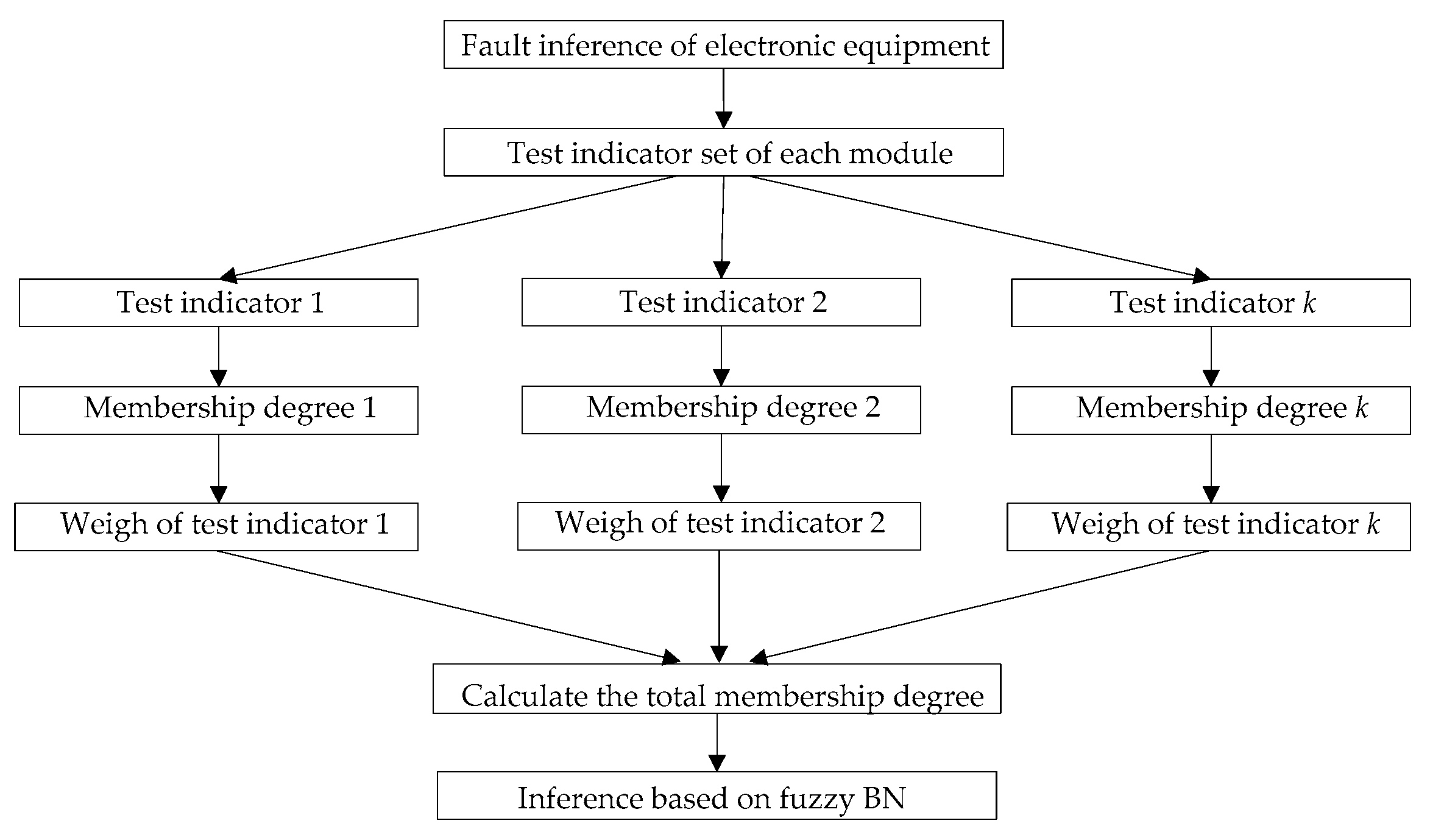
2.2.2. Indicator for Fault Detection
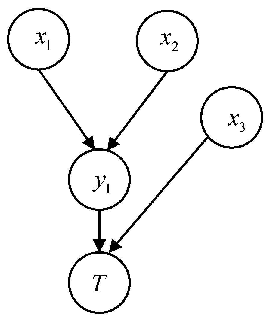
2.3. Directed Edge A of FRM
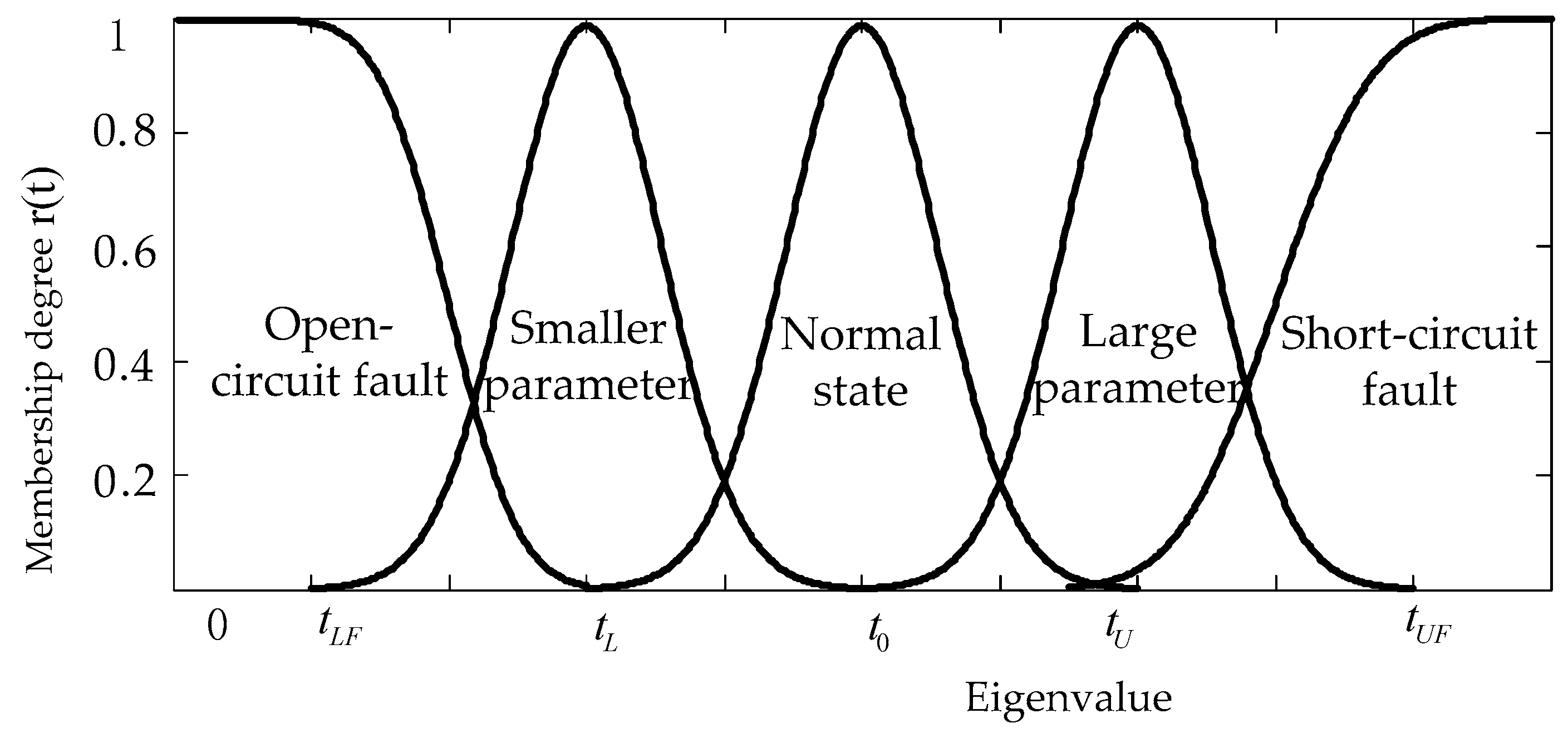
2.4. Fuzzy Membership Degree of Nodes in Fault State with Multiple Test Indicators
3. Multi-State Fuzzy BN
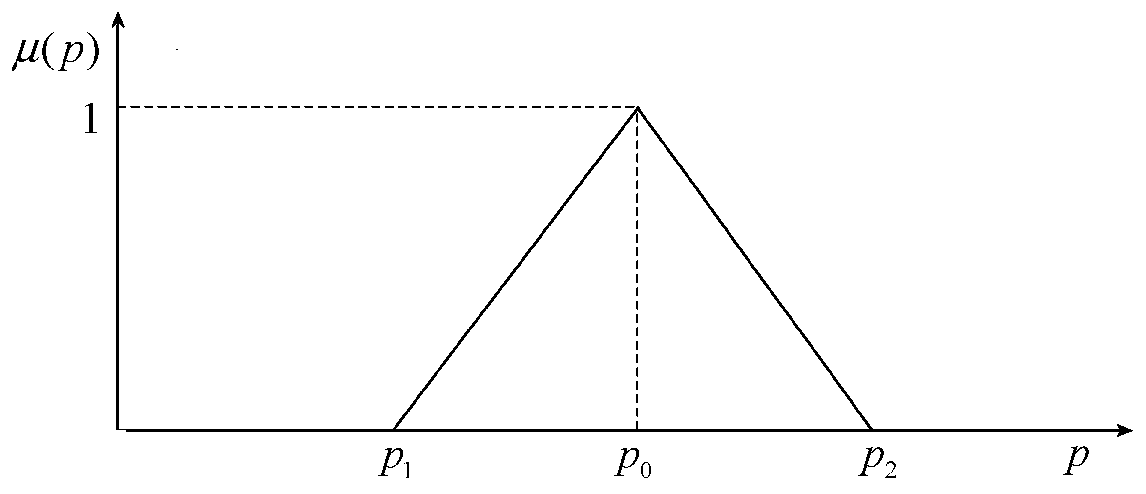
3.1. Fuzziness of Prior Probability of Faults of Nodes
3.2. CPT of Fuzzy BN
3.3. Inference Based on Fuzzy BN
- (1)
- Inference of Fuzzy Fault State of Leaf Nodes
- (2)
- Fuzzy fault inference of faults of root nodes
4. Example Analysis
4.1. Calculation of Interval of Fault Probability of Leaf Nodes
4.2. Calculation of Posteriori Probability of Root Nodes
5. Conclusions
- (1)
- In view of how to determine fault state through multiple test indicators of test modules, the normal membership function of a single parameter is proposed; Experts assign the weights of test indicators for normalization of membership degree. In order to assist test personnel in understanding and programming, five fault states are divided according to test indicators.
- (2)
- In inference based on BN, due to limited samples of electronic modules, according to statistical values of the samples and experts’ experience and tables of prior probability and conditional probability, fuzzy inference was performed by using triangular membership function.
- (3)
- Based on multi-state fuzzy BN, the bidirectional inference of faults could be conducted to speculate fault state of leaf nodes for fault verification and calculate posterior probability of fault of root nodes, so as to find fault source and rapidly locate faults.
Author Contributions
Funding
Conflicts of Interest
References
- Si, X.-S.; Wang, W.; Hu, C.-H.; Zhou, D.-H. Remaining useful life estimation—A review on the statistical data driven approaches. Eur. J. Oper. Res. 2011, 213, 1–14. [Google Scholar] [CrossRef]
- Gao, Z.; Cecati, C.; Ding, S.X. A Survey of Fault Diagnosis and Fault-Tolerant Techniques—Part I: Fault Diagnosis with Model-Based and Signal-Based Approaches. IEEE Trans. Ind. Electron. 2015, 62, 3757–3767. [Google Scholar] [CrossRef]
- Nguyen, T.L.; Djeziri, M.; Ananou, B.; Ouladsine, M.; Pinaton, J. Fault prognosis for batch production based on percentile measure and gamma process: Application to semiconductor manufacturing. J. Process. Control. 2016, 48, 72–80. [Google Scholar] [CrossRef]
- Benmoussa, S.; Djeziri, M.A. Remaining useful life estimation without needing for prior knowledge of the degradation features. IET Sci. Meas. Technol. 2017, 11, 1071–1078. [Google Scholar] [CrossRef]
- Chu, X.; Luan, S.; Wen, Q. Defects Analysis and Strategy Seeking of Automatic Test and Diagnosis System (ATDS) for Airborne Equipment. In Proceedings of the First Symposium on Aviation Maintenance and Management-Volume II; Springer: Berlin/Heidelberg, Germany, 2014. [Google Scholar]
- Butz, C.J.; Oliveira, J.S.; Madsen, A.L. Bayesian network inference using marginal trees. Int. J. Approx. Reason. 2016, 68, 127–152. [Google Scholar] [CrossRef]
- Gendelman, R.; Xing, H.; Mirzoeva, O.K.; Sarde, P.; Curtis, C.; Feiler, H.S.; McDonagh, P.; Gray, J.W.; Khalil, I.; Korn, W.M. Bayesian network inference modeling identifies TRIB1 as a novel regulator of cell-cycle progression and survival in cancer cells. Cancer Res. 2017, 77, 1575–1585. [Google Scholar] [CrossRef]
- Li, X.; Li, H.; Qin, L.; Xu, X. Bayesian network inference on departure time choice behavior. In Proceedings of the International Conference on Electrical and Information Technologies for Rail Transportation, Changsha, China, 20–22 October 2017; Springer: Singapore, 2017. [Google Scholar]
- Bouzembrak, Y.; Camenzuli, L.; Esmée, J.; van der Fels-Klerx, H.J. Application of Bayesian networks in the development of herbs and spices sampling monitoring system. Food Control. 2017, 83, 38–44. [Google Scholar] [CrossRef]
- Yin, X.; Jiang, C.; Li, B. Fault diagnosis based on fault tree and Bayesian network for pure electric trucks. In Proceedings of the Technology, Networking, Electronic and Automation Control Conference, Chengdu, China, 15–17 December 2017; IEEE: Piscataway, NJ, USA, 2018. [Google Scholar]
- Islam, M.M.M.; Kim, J.; Khan, S.A.; Kim, J.-M. Reliable bearing fault diagnosis using Bayesian inference-based multi-class support vector machines. J. Acoust. Soc. Am. 2017, 141, EL89. [Google Scholar] [CrossRef]
- Chen, X.; Liu, Y.; Huang, J.; Chen, X. Fault diagnosis of landing gear system based on Bayesian network inference. Comput. Meas. Control. 2016, 24, 24–28. [Google Scholar]
- Wang, D.; Tian, Y.; Ye, S.F.; Liu, Q. Fault Diagnosis of the Foundation Brake Rigging System Based on Fault Tree and Bayesian Network. Key Eng. Mater. 2016, 693, 1734–1740. [Google Scholar] [CrossRef]
- Wang, H.; Sha, S. The intelligent fault diagnosis based on Bayesian network inference algorithm solution. Appl. Mech. Mater. 2015, 727–728, 884–887. [Google Scholar] [CrossRef]
- Zhai, S.; Lin, S.Z. Bayesian networks application in multi-state system reliability analysis. Appl. Mech. Mater. 2013, 347–350, 2590–2595. [Google Scholar] [CrossRef]
- Torres-Toledano, J.; Sucar, L.E. Bayesian networks for reliability analysis of complex systems. In Proceedings of the International Conference on Grey Systems and Intelligent Services, Stockholm, Sweden, 8–11 August 2017; IEEE: Piscataway, NJ, USA, 2017. [Google Scholar]
- Cai, B.; Liu, Y.; Xie, M. A dynamic-Bayesian-network-based fault diagnosis methodology considering transient and intermittent fault. IEEE Trans. Autom. Sci. Eng. 2017, 14, 276–285. [Google Scholar] [CrossRef]
- Cai, B.; Huang, L.; Xie, M. Bayesian Networks in Fault Diagnosis. IEEE Trans. Ind. Inf. 2017, 13, 2227–2240. [Google Scholar] [CrossRef]
- Cai, Z.Q.; Sun, S.D.; Si, S.B.; Wang, N. Modeling of failure prediction Bayesian network based on FMECA. Syst. Eng. Theory Pract. 2013, 33, 187–193. [Google Scholar]
- Chen, T.T.; Leu, S.S. Fall risk assessment of cantilever bridge projects using Bayesian network. Saf. Sci. 2014, 70, 161–171. [Google Scholar] [CrossRef]
- Said, A.B.; Shahzad, M.K.; Zamai, E.; Hubac, S.; Tollenaere, M. Experts’ knowledge renewal and maintenance actions effectiveness in high-mix low-volume industries, using Bayesian approach. Cognit. Technol Work. 2016, 18, 193–213. [Google Scholar] [CrossRef]
- Li, Z.; Xu, T.; Gu, J.; Dong, Q.; Fu, L. Reliability modeling and analysis of a multi-state element based on a dynamic Bayesian network. R. Soc. Open Sci. 2018, 5, 315–329. [Google Scholar] [CrossRef]
- Doguc, O.; Ramirez-Marquez, J.E. A generic method for estimating system reliability using Bayesian networks. Reliab. Eng. Syst. Saf. 2017, 94, 542–550. [Google Scholar] [CrossRef]
- Wang, Y.; Liu, Y.; Khan, F.; Imtiaz, S. Semiparametric PCA and bayesian network based process fault diagnosis technique. Can. J. Chem. Eng. 2017, 95, 1800–1816. [Google Scholar] [CrossRef]
- Li, H.-T.; Jin, G.; Zhou, J.-L. Survey of Bayesian network inference algorithms. Syst. Eng. Electr. 2008, 30, 935–939. [Google Scholar]
- Álvaro, C.; Gonzalez-Ordás, J.; García-Algarra, J.; Arozarena, P.; Garijo, M. A multi-agent system with distributed Bayesian reasoning for network fault diagnosis. Adv. Pract. Appl. Agents Multi Agent Syst. 2011, 88, 113–118. [Google Scholar]
- Xiaoli, X.U.; Liu, X.; Jiang, Z.; Ren, B. Multi-sensor distributed fault detection method based on subjective Bayesian reasoning. J. Mech. Eng. 2015, 51, 91–99. [Google Scholar]
- Gao, X.Q.; Du, J.; Zhang, Y.P. Reasoning method of fuzzy Bayesian network for CNC machine tool fault based on bucket elimination. Aviat. Precis. Manuf. Technol. 2016, 52, 14–18. [Google Scholar]
- de-Zhong, M.; Zhou, Z.; Yu, X.-Y. Reliability analysis of multi-state Bayesian networks based on fuzzy probability. Syst. Eng. Electr. 2012, 34, 2607–2611. [Google Scholar]
- Hefei University. Bucket-tree based algorithm for automated reasoning. Comput. Sci. 2013, 40, 211–217. [Google Scholar]
- Yang, J.; Xiao, X.; Guo, J. Gray prediction model of normal distribution interval grey number. Control Decis. 2015, 30, 1711–1716. [Google Scholar]
- Zhang, R.; Zhang, L.; Wang, X. Research on reliability of multi-state system based on interval triangular fuzzy Bayesian network. China Mech. Eng. 2015, 26, 1092–1097. [Google Scholar]
- He, Q.; Zha, Y.; Zhang, R.; Sun, Q.; Liu, T. Reliability analysis for multi-state system based on triangular fuzzy variety subset Bayesian networks. Eksploat. Niezawodn. Maint. Reliab. 2017, 19, 152–165. [Google Scholar] [CrossRef]


| … | … | |||||
|---|---|---|---|---|---|---|
| 0 | 0 | … | 0 | … | ||
| … | … | … | … | … | … | … |
| 1 | 1 | … | 1 | … |
| 0 | 0 | 1 | 0 | 0 |
| 0 | 0.5 | {0.1, 0.2, 0.3} | {0.2, 0.3, 0.4} | 0.5 |
| 0 | 1 | 0 | 0 | 1 |
| 0.5 | 0 | {0.3, 0.4, 0.5} | {0.3, 0.4, 0.5} | {0.1, 0.2, 0.3} |
| 0.5 | 0.5 | {0, 0.1, 0.2} | {0.1, 0.2, 0.3} | 0.7 |
| 0.5 | 1 | 0 | 0 | 1 |
| 1 | 0 | 0 | 0 | 1 |
| 1 | 0.5 | 0 | 0 | 1 |
| 1 | 1 | 0 | 0 | 1 |
| 0 | 0 | 1 | 0 | 0 |
| 0 | 0.5 | {0.3, 0.4, 0.5} | {0.3, 0.4, 0.5} | 0.2 |
| 0 | 1 | 0 | 0 | 1 |
| 0.5 | 0 | {0.5, 0.6, 0.7} | {0.2, 0.3, 0.4} | {0, 0.1, 0.2} |
| 0.5 | 0.5 | 0.3 | {0.4, 0.5, 0.6} | {0.1, 0.2, 0.3} |
| 0.5 | 1 | 0 | 0 | 1 |
| 1 | 0 | 0 | 0 | 1 |
| 1 | 0.5 | 0 | 0 | 1 |
| 1 | 1 | 0 | 0 | 1 |
| Fault State of Node | Value of Fault Probability | ||
|---|---|---|---|
| 0 | 0.5 | 1 | |
| {0.3, 0.4, 0.5} | {0.3, 0.5, 0.7} | {0, 0.1, 0.15} | |
| {0, 0.1, 0.2} | {0.1, 0.2, 0.3} | {0.5, 0.7, 0.8} | |
| {0, 0.1, 0.2} | {0, 0.1, 0.2} | {0.6, 0.8, 0.9} | |
| {0, 0.1, 0.2} | {0.1, 0.2, 0.3} | {0.5, 0.7, 0.8} | |
| 0.714 | 0 | 0.774 | 1 | |
| 0.556 | 0 | 0.826 | 1 | |
| 0.263 | 0 | 0.156 | 1 |
© 2019 by the authors. Licensee MDPI, Basel, Switzerland. This article is an open access article distributed under the terms and conditions of the Creative Commons Attribution (CC BY) license (http://creativecommons.org/licenses/by/4.0/).
Share and Cite
Wang, L.; Zhou, D.; Zhang, H.; Tian, H.; Zou, C.; Wang, X. Fault Inference of Electronic Equipment Based on Multi-State Fuzzy Bayesian Network. Appl. Sci. 2019, 9, 4248. https://doi.org/10.3390/app9204248
Wang L, Zhou D, Zhang H, Tian H, Zou C, Wang X. Fault Inference of Electronic Equipment Based on Multi-State Fuzzy Bayesian Network. Applied Sciences. 2019; 9(20):4248. https://doi.org/10.3390/app9204248
Chicago/Turabian StyleWang, Ling, Dongfang Zhou, Hao Zhang, Hui Tian, Caihong Zou, and Xiushan Wang. 2019. "Fault Inference of Electronic Equipment Based on Multi-State Fuzzy Bayesian Network" Applied Sciences 9, no. 20: 4248. https://doi.org/10.3390/app9204248
APA StyleWang, L., Zhou, D., Zhang, H., Tian, H., Zou, C., & Wang, X. (2019). Fault Inference of Electronic Equipment Based on Multi-State Fuzzy Bayesian Network. Applied Sciences, 9(20), 4248. https://doi.org/10.3390/app9204248