Article

Labeled Multi-Bernoulli Filter Joint Detection and Tracking of Radar Targets

National Key Laboratory of Science and Technology on ATR, College of Electronic Science, National University of Defense Technology, Changsha 410073, China
*
Author to whom correspondence should be addressed.
Appl. Sci. 2019, 9(19), 4187; https://doi.org/10.3390/app9194187
Submission received: 8 August 2019 / Revised: 27 September 2019 / Accepted: 29 September 2019 / Published: 8 October 2019
(This article belongs to the Special Issue Multi-Channel and Multi-Agent Signal Processing)

Abstract

:
A labeled multi-Bernoulli (LMB) filter is presented to jointly detect and track radar targets. A relevant LMB filter is recently proposed by Rathnayake which assumes that the measurements of different targets do not overlap, leading to the favorable separable likelihood assumption. However, new or close tracks often violate the assumption and lead to a bias in the cardinality estimate. To address this problem, a one-to-one association method between measurements and tracks is proposed. In our method, any target only corresponds to its associated measurements and different tracks have little mutual interference. In addition, an approximate method for calculating the point spread function of radar is developed to improve the computational efficiency of likelihood function. The simulation under low signal-to-noise ratio scenario with closely spaced targets have demonstrated the effectiveness and efficiency of the proposed algorithm.

1. Introduction

Multi-target tracking based on multi-target Bayes filter makes an important contribution to capturing and maintaining the awareness of the environment [1,2]. Multi-target Bayes filter is usually computationally intractable [3] by simply extending the classic single-target Bayes filters [4] for multi-target case. With the development of the emerging random finite set (RFS) theory, tremendous efforts have been devoted to investigating various approximate multi-target Bayes filters [5,6,7,8], including probability hypothesis density (PHD) filter, cardinalized PHD (CPHD) filter and multi-Bernoulli (MB) filter, and their various revised versions. In order to integrate track management into the filtering scheme, the so-called generalized labeled multi-Bernoulli (GLMB) filter and labeled multi-Bernoulli (LMB) filter were proposed [9,10,11]. Most of these filters are based on the standard multi-target observation model which assumes that one target generates at most one measurement and so any measurement corresponds to at most one target [12]. However, in many scenarios, the observation models are nonstandard and cannot be modeled by standard multi-target likelihood function, for example, track before detect (TBD) in video [13,14], superpositional sensors [15,16,17], unresolved target tracking [18] and extended target tracking [19].
As a typical application of the nonstandard observation model, the TBD algorithm of radar targets [20,21,22,23,24,25] works with the raw radar data directly, and detects and tracks the targets jointly, so it is suitable for application in a low signal-to-noise ratio (SNR) scenario. The observation model for radar sensor is called a generic observation model (GOM) [20,26]. This is because the measurements affected by different target point spread functions may overlap. The joint likelihood function for the GOM cannot be denoted as the product of each target likelihood function and so it is typically referred to as inseparable likelihood [20]. However, for computational efficiency, it could be assumed that the measurements affected by different targets do not overlap and then the separable likelihood could be derived [20,27].
References [27,28] proposed the MB filter and the LMB filter for the GOM under the assumption of the separable likelihood which are called the S-MB-GOM filter and the S-LMB-GOM filter, respectively. Both filters are computational efficiently but the cardinality estimate bias easily occurs when the separable likelihood assumption is violated. Firstly, due to the influence of new or close tracks, the measurements generated by a target may be associated with multiple tracks which causes an increase of cardinality estimate. Secondly, the measurements generated by multiple closely spaced targets may only be associated with a track due to merging [12] which causes a decrease of cardinality estimate.
To avoid the problem, References [20,26] proposed the GLMB filter and the group LMB filter for the GOM, which are called the GLMB-GOM filter and the G-LMB-GOM filter, respectively. Both filters adapt to inseparable likelihood and improve the tracking performances for radar. However, the implementations of both filters require high-dimensional particle sampling, so the calculation amounts are intensive.
In our paper, we propose a one-to-one correspondence method between measurements and tracks to overcome the cardinality estimate bias of the S-LMB-GOM filter [28]. Further, to improve the computational efficiency of the S-LMB-GOM filter, we propose an approximate method to calculate the point spread function according to its property analysis. The  Sequential Monte Carlo (SMC) approximation method has been used to implement our S-LMB-GOM filter. The  performance is verified by a scenario with closely spaced targets in low SNR and compared with the G-LMB-GOM filter. The S-LMB-GOM filter applying the proposed method can significantly reduce the probability of violating the separable likelihood assumption and drastically reduce the computational complexity without loss of performance compared with the G-LMB-GOM filter.
The rest of the paper is structured as follows. We review the basic definitions of LMB RFS and introduce the generic observation model for radar sensor in Section 2. In Section 3, the S-LMB-GOM filter is introduced, and then a one-to-one correspondence method and an approximate method to calculate point spread function are proposed. Section 4 is the simulation results of radar target detection and tracking under nonlinear motion model. The conclusion is given in Section 5.

2. Backgound

2.1. LMB RFS

The label space denoted as L contains a countable number of distinct labels. The unlabeled target state space is denoted as X . The labeled single target state is denoted as x = x , , where x X denotes the target state and L denotes the label. The labeled multi-target state is denoted as X = { x 1 , , x i , , x X } , where X denotes the cardinality of the multi-target, x i denotes a labeled single target state and  X X × L . The generalized Kronecker delta function and the inclusion function can be defined as:
δ Y ( X ) 1 , X = Y 0 , otherwise , 1 Y ( X ) 1 , X Y 0 , otherwise .
Define a projection L : X × L L to make L ( x ) = and L ( X ) = { L ( x ) : x X } . Δ ( X ) = δ | X | ( | L ( X ) | ) is the indicator function of distinct labels. When X has distinct labels, Δ ( X ) = 1 . The inner product of f x and g x on X × L is defined as f , g f x g x d x . The multi-target exponential function is defined as
h X 1 , X = x X h ( x ) , X .
The LMB distribution of an LMB RFS with the parameter form π = { ( r , p ) } L is
π X = Δ X ω L X p X
where r is the existence probability of the target x and  p = p x is the probability density of the target x . The weight ω ( I ) of the hypothesis I = { 1 , , | I | } is
ω ( I ) = i L ( 1 r i ) I 1 L ( ) r 1 r .

2.2. The Observation Model and Likelihood Function of Radar

The range-azimuth-Doppler image of the echo power signal is used as the raw radar measurements [20,21]. The measurements per frame can be denoted as a three dimensional matrix after sampling. Each element in the matrix denotes a measurement and the coordinate of measurement cell i can be denoted as c i x r m , b n , d q , where r m , b n and d q denote the range, azimuth and Doppler cells, respectively. i = m , n , q is the index of cell i. The index set of the measurements affected by the target x is called the target template and denoted by T x . i T x denotes that the measurement in cell i is affected by x . The setting of T x is detailed in Section 3.4.
The measurement matrix can also be denoted as a vector form Υ = z 1 , , z i , , z m z , where m z is the number of the measurements, z i z i X is the power signal in cell i and  X is the multi-target state. The measurement z i can be denoted as [20,25]
z i = z A i 2 = x X 1 T x i A x h A i x + w n i 2
where z A i is the received complex signal in cell i and  w n i denotes a zero-mean complex Gaussian white noise with a variance of 2 σ w n 2 . A x is a complex amplitude. x X 1 T x i denotes that the signal in cell i is the sum generated by X , so the signal in each cell may affected by all x ( x X ).
h A i ( x ) denotes the signal generated by the point spread function of the target x . The expression is (according to the point spread function formula of Reference [21], we assume that L r = 1 R , L d = 1 D , L b = 1 B )
h A i x = exp ( r m r x 2 2 R 2 b n b x 2 2 B 2 d q d x 2 2 D 2 )
where
r x = p x 2 + p y 2 ,
b x = a t a n 2 p y , p x ,
d x = p x p ˙ x + p y p ˙ y / r x ,
R , B and D denote the range, azimuth and Doppler resolution of radar, respectively. p x , p y T and p ˙ x , p ˙ y T denote the position and speed of x in the state space, respectively. r x , b x and d x denote the range, azimuth and Doppler positions relating to x , respectively. Note that r x , b x and d x are continuous while r m , b n and d q are discrete sampling in the measurement space.
In the following, we construct the likelihood function of the radar observation model. The estimated value of the measurement z i in cell i is denoted by z ^ i and  z ^ i can be written as [25]
z ^ i = z ^ A i 2 x X 1 T x i A ¯ h A i x 2 .
When z ^ A i 0 , z i / σ w n 2 subjects to a noncentral χ 2 distribution with 2 degrees of freedom. The  probability density of z i is
P z i | X = 1 2 exp z i + z ^ i 2 σ w n 2 I 0 z i z ^ i σ w n 2 , z i > 0 0 , z i < 0 .
where I 0 u is the first kind modified Bessel function with 0 order. When z ^ A i = 0 ( only with noise), z i / σ w n 2 subjects to a central χ 2 distribution with 2 degrees of freedom. The probability density of z i is
P z i | X = 1 2 exp z i 2 σ w n 2 , z i > 0 0 , z i < 0 .
Dividing Equation (12) by Equation (11), we can obtain that the likelihood ratio function of cell i  is
l z i | X = exp z ^ i 2 σ w n 2 I 0 z i z ^ i σ w n 2 , z i > 0 0 , z i < 0 .
The likelihood function of the measurement vector Υ can be written as
g Υ | X = f Υ i x X T x l z i | X
where f Υ = 1 i m z 0.5 exp 0.5 σ w n 2 1 z i denotes the likelihood function only with noise. g Υ | X cannot be denoted as a product form of each target likelihood function so it is called the inseparable likelihood.
If we assume that the measurements generated by different targets do not overlap and any measurement is most affected by one target. Therefore, there is at most one item in z ^ i ,
z ^ i = z ^ A i 2 = 1 T x i A ¯ h A i x 2 .
Further, the second term of Equation (14) can be simplified to
i x X T x l z i | X = x X i T x l z i | x .
The likelihood function g Υ | X can be denoted as the product of the likelihood function of each target x so it is called the separable likelihood. The expression can be written as
g Υ | X = f Υ x X g Υ x ,
g Υ x = i T x l z i | x .

2.3. Multi-Target Bayes Filter

The label space of the birth targets at time k is L k , the label space of the targets (including the targets prior to k 1 ) at k 1 is L 0 : k 1 and  L 0 : k = L 0 : k 1 L k denotes the label space at k. The multi-target state at k is X k X × L 0 : k and the multi-target state at k 1 is X k 1 X × L 0 : k 1 . The measurement vector at time k is Υ k . The prediction and update for the multi-target Bayes filter can be written as [6]
π k | k 1 X k = f k | k 1 X k | X k 1 π k 1 X k 1 δ X k 1
π k X k = g k Υ k | X k π k | k 1 X k g k Υ k | X k π k | k 1 X k δ X k
where π k 1 is the multi-target prior, π k | k 1 is the predicted multi-target posterior, f k | k 1 is the multi-target Markov transition density, g k is the multi-target likelihood function and  π k is the multi-target posterior density at k. The integral is the set integral. For simplicity, we define L L 0 : k 1 , B L k , L + L 0 : k , π π k 1 , π + π k | k 1 , π ¯ π k , g g k and f f k | k 1 .

3. The S-LMB-GOM Filter

In this section, firstly, we introduce the prediction and the update of the S-LMB-GOM filter; Secondly, a method to overcome the cardinality estimate bias of the filter is proposed. Thirdly, we  analyze the property of the point spread function and set the size of T x . Finally, an approximate method for calculating point spread function is proposed to improve the efficiency.

3.1. Prediction

Given that the multi-target prior is an LMB distribution denoted as π = { ( r , p ) } L . P s x denotes the survival probability from k 1 to k. The Markov density f + x + | x , denotes the transiting probability from k 1 to k. The density of the newborn targets is an LMB distribution denoted as π = { ( r B , p B ) } B . From References [8,11], the predicted probability density is
π + = r + , s , p + , s L r B , p B B = r + , p + L +
where
r + , s = η s r , η s = P S · , , p · , ,
p + , s x + = P s · f + x + | · , , p · , η s ,
p + x + = 1 L p + , s x + + 1 B p B x + .

3.2. Update

The predicted multi-target posterior π + = { ( r + , p + ) } L + is an LMB distribution. π + has the form of Equation (3) and can be denoted as { ( W + I + , x X + p + ) } I + L + . I + is the label set of X + and also denotes a possible multi-target hypothesis. W + I + denotes the existence probability of the hypothesis. Under the separable likelihood assumption, we can obtain that g Υ | X + = f Υ x X + g Υ x .
From Reference [28], the multi-target posterior density π ¯ can be written as
π ¯ = r ¯ + , p ¯ + L +
where
r ¯ + = r + η Υ 1 r + + r + η Υ ,
p ¯ + x = g Υ x p + x η Υ ,
η Υ = g Υ ( · , ) , p + ( · , ) .
Therefore, when the prior is an LMB distribution, the multi-target predicted density and posterior density are both LMB distributions, so the LMB distribution is the conjugate prior for the S-LMB-GOM filter [27,28]. Each hypothesized track of the S-LMB-GOM filter is predicted and updated independently so the filter is efficient.

3.3. A Method to Overcome the Cardinality Estimate Bias

3.3.1. The Reason of the Bias

New birth hypothesized tracks often violate the separable likelihood assumption [20] which leads to a cardinality estimate bias for the S-LMB-GOM filter.
Each hypothesized track is updated independently and the probability density of each track is approximated by a group of particles in the state space. As shown in the Figure 1, when a new target x is born, the particle group of the hypothesized track 1 surrounds the target x and then x is subsequently tracked by track 1 . The particle group of 1 always surrounds x until the target dies. If the particle group of another birth hypothesized track 2 also surrounds the target before the target died, the target x will be detected again and an increase of cardinality estimate will occur.
The reason is that the target x is surrounded by multiple particle groups of different tracks which makes the measurements affected by the target x associate with multiple tracks, then the target will be detected repeatedly. Eventually, a cardinality estimate bias occurs.

3.3.2. The One-to-One Correspondence Method

Motivated by the standard LMB filter, we propose a one-to-one correspondence method between measurements and tracks to overcome the problem of the cardinality estimate bias. The idea of our method is similar with the Nearest Neighbor (NN) method [29]. The difference is that our method matches the maximum likelihood but the NN method matches the smallest distance.
The method can be summarized as Algorithm 1. We update the predicted track in order of existence probability r + to prevent the new birth predicted tracks from interfering with the surviving predicted tracks. Given that the predicted track 1 update first and after update the existence probability r ¯ + 1 is greater than the detection threshold λ (e.g., λ = 0.5), the hypothesized track 1 is considered a true track and has tracked a target x . Still as shown in the Figure 1, the target x can be approximated by the particle x ^ with the maximum likelihood in the particle group of track 1 . The associated measurements by T ( x ) are reset to noise, where T ( x ) is approximated by T ( x ^ ) . This  operation makes the track 1 only correspond to the associated measurements by T x . The  setting of T x is detailed in Section 3.4. Then, another predicted track 2 is updated and cannot track the same target x again due to the resetting of the associated measurements. Therefore, the overlapped particle groups will no longer lead to a repeated cardinality estimate.
Algorithm 1 One-to-one correspondence method
1. Descending sort: r + = sort L + ( r + , descend ) .
2: Update in order of r + to get r ¯ + and p ¯ + ( x ) .
    If r ¯ + λ
         x ^ = max x X (compute-likelihood( Z , x )).
         x x ^ .
         Z = reset-noise ( Z , T x ) .
    end
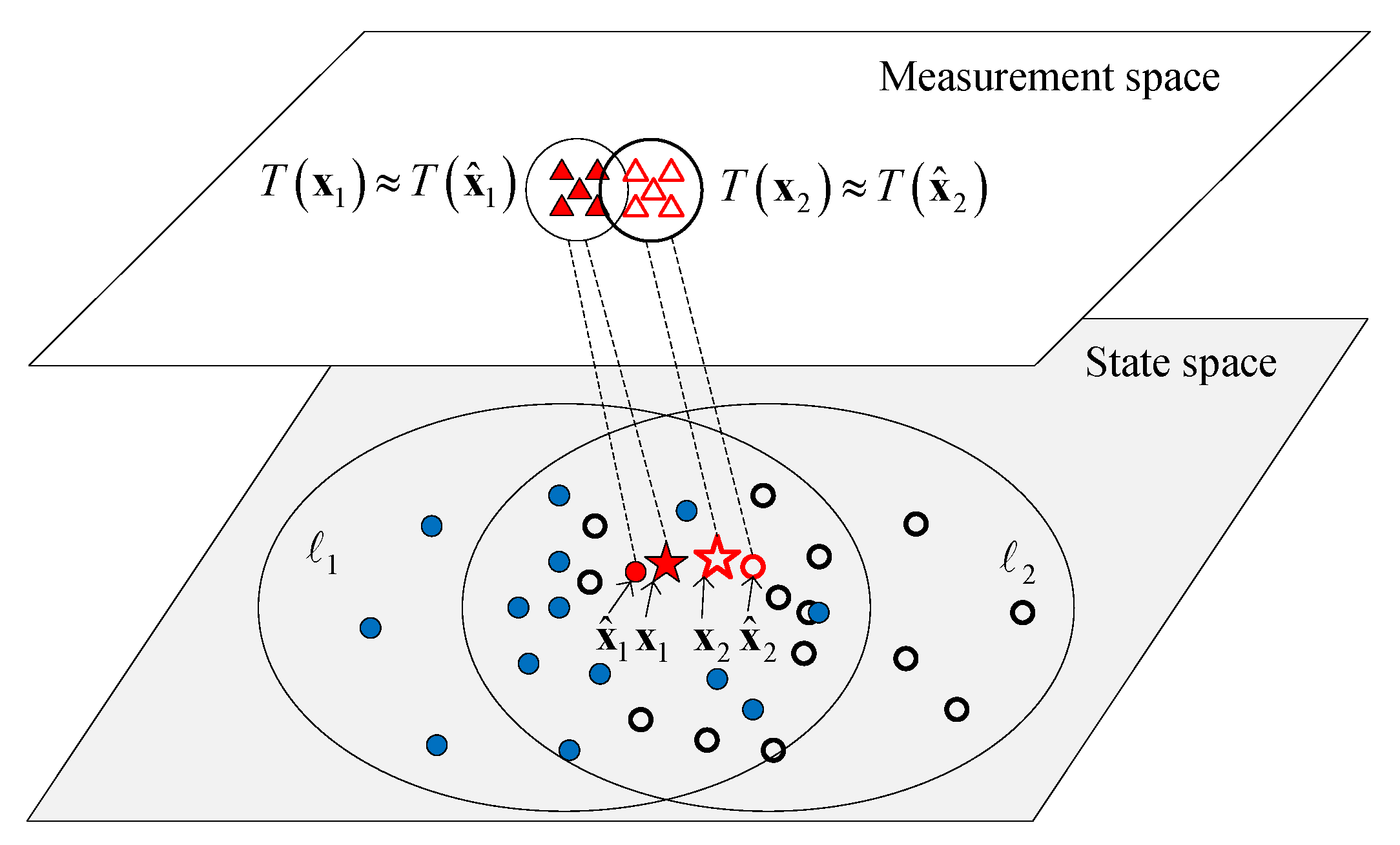
When the two targets x 1 and x 2 are closely spaced and the templates T x 1 and T x 2 are partially overlapped as shown in the Figure 2, the one-to-one correspondence method can work properly. After update of the track 1 , the target x 1 is associated with track 1 and the associated measurements by T x 1 are reset to noise where T ( x 1 ) T ( x ^ 1 ) . If the setting range of T x 1 is small enough and T x 1 do not include the peak region of the likelihood function of the target x 2 , then x 2 can be distinguished at the update step, because the peak region of likelihood function roughly corresponds to a target position and determines the existence probability of the target.

3.3.3. The Analysis and Performance of the Proposed Method

The new birth probability is usually smaller than the surviving probability. We update the predicted track in order of existence probability, that is, let the surviving tracks update firstly. This is to prevent the new birth predicted tracks from interfering with the survived predicted tracks and ensure the continuity of the tracks.
In essence, the one-to-one correspondence method reduces the probability of violating the separable likelihood assumption. The particle groups are in the state space and the sets T ( · ) of the associated measurements are in the measurement space. As seen in the Figure 1 and Figure 2, the particle group of each track has a large coverage to prevent particle depletions, while the coverage of the associated measurements T ( · ) can be set small. Therefore, the probabilities of the mutual interference of different tracks get smaller after applying the one-to-one correspondence method. Further, the method can reduce the negative effect of separable likelihood assumption but cannot completely eliminate the negative effect.
For radar, when the target planar positions overlap completely, there is usually a difference in the Doppler cell and the targets can still be considered closely spaced. Even if the Doppler cell is also temporarily the same and the one-to-one correspondence method will cause a bias in the cardinality estimate temporarily. Then we can set a low intercept threshold so that the hypothesized tracks can survive through the completely overlapped region and wait for the next update. Therefore, the one-to-one correspondence method still can work.
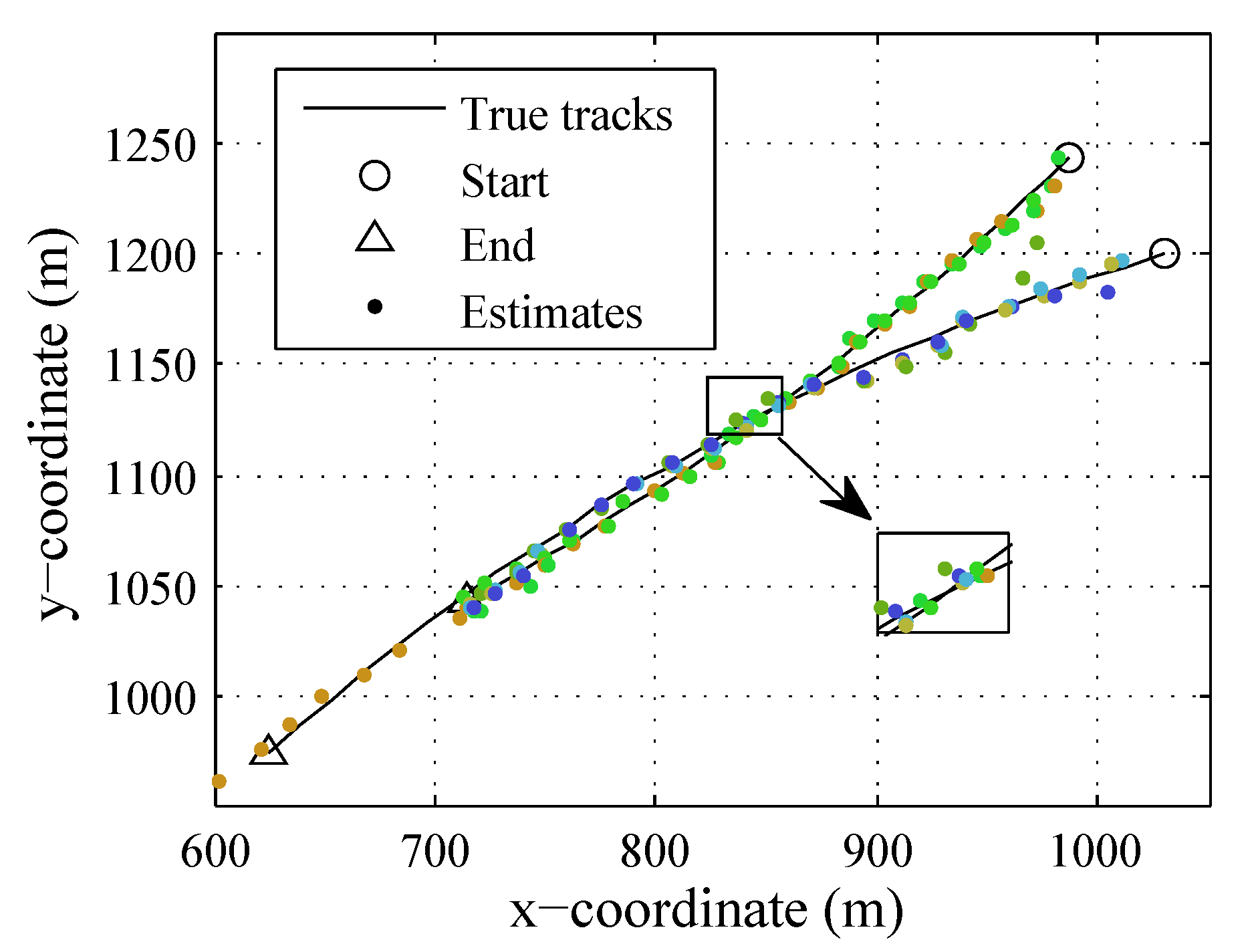
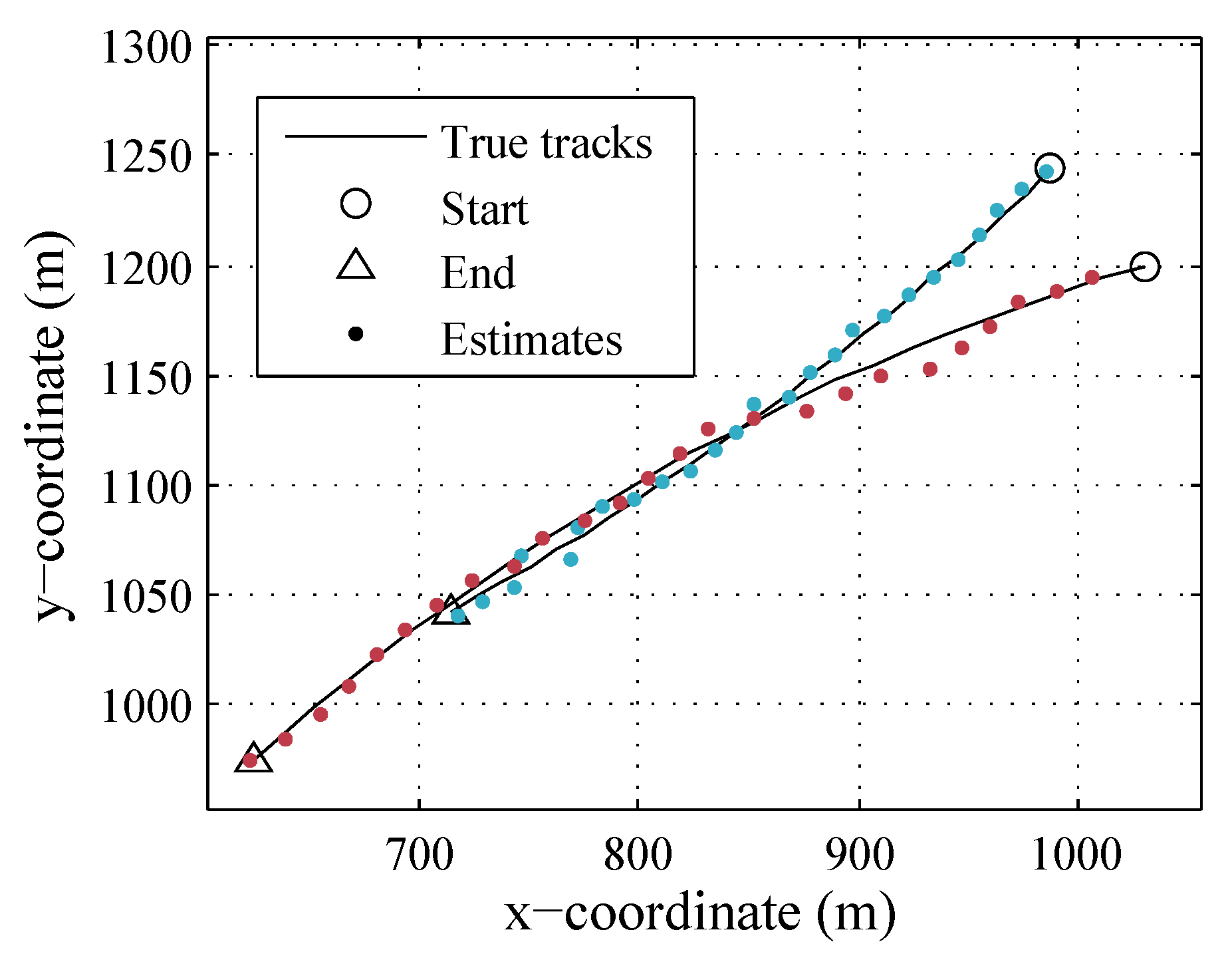
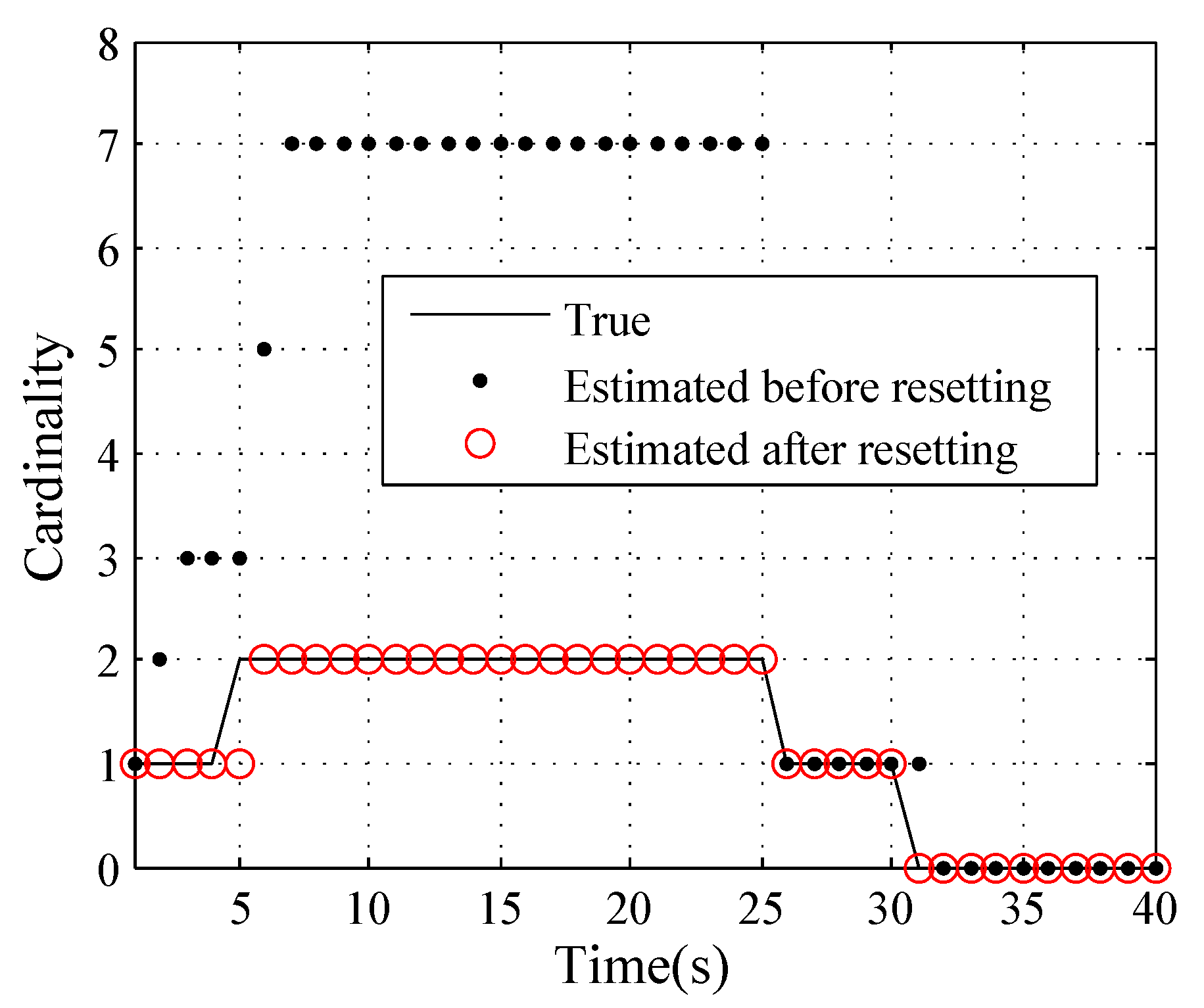
A scenario with two closed targets has been used for our comparisons of two cases: without applying the one-to-one correspondence method between measurements and tracks or with applying the proposed method. Figure 3 shows the true trajectory and the estimated trajectory without applying the proposed method. Figure 4 shows the true trajectory and the estimated trajectory with applying the proposed method. Figure 5 shows the true cardinality and the estimated cardinality without and with applying the proposed method. From Figure 3 and Figure 5, it can be seen without applying the proposed method that the estimated cardinality is 7 from 7th to 25th frame while in fact there are only two targets and the estimated cardinality is 1 to 3 from 1th to 4th frame, while in fact there is only one target. From Figure 4 and Figure 5, it can be seen with applying the proposed method that the trajectory and the cardinality is estimated accurately. Therefore, in the subsequent comparisons with other methods in Section 4, we have applied the one-to-one correspondence method between measurements and tracks.

3.4. The Property Analysis and the Set of the Point Spread Function

We analyze the property of the point spread function h A i x defined in Equation (6) and set the size of T x .
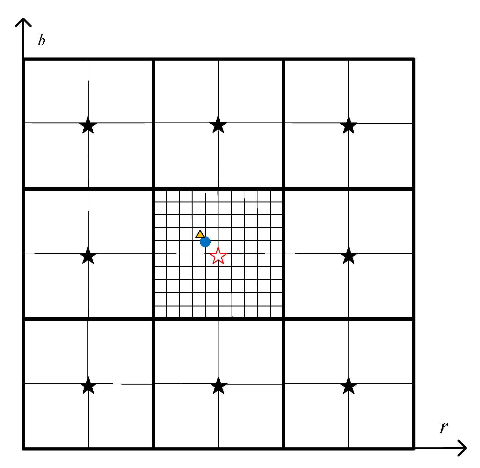
We assume that R = 5 m, B = π / 180 rad, D = 1 m/s in Equation (6) and c 0 = R , B , D . The sampling interval of the measurement space is equal to the resolution. The corresponded range, azimuth and Doppler cell of the target x is denoted as c t x = r x , b x , d x and c t x is not necessarily the position of a measurement cell as it is not necessarily located in the sampling position. Find the closest cell c i 0 x to c t x in the measurement space, then find the nearest k cells around cell c i 0 x in each dimension to construct the set C x where C x = c i x : i T x is the corresponded position cell set of the index set T x and c i x = r m , b n , d q . C x is a k × k × k matrix and falls within a certain distance from c i 0 x . A simple example to show the relations of different cells is given in Figure 6. T x is the index set of C x and contains k 3 index elements. Define the confidence level β as
β = i T x 1 U i h A i x i U 1 U i h A i x
where U represents the complete index set of the measurement space and 0 β 1 . When β is close to one, we think that T x can replace U almost without loss.
From the result of Table 1, the cell number k of C x in each dimension can be set to 9 when the simulation data is generated and T x contains 729 index elements; the cell number k of C x can be set to 5 to reach a compromise between computational efficiency and accuracy when calculating likelihood function and T x contains 125 index elements; the cell number k of C x can be set to 2 or 3 to reduce the impact on the other close targets when resetting the associated measurements into noises and T x contains 8 or 27 index elements.

3.5. An Approximate Method for Calculating Point Spread Function

The idea for fast calculation of point spread function is approximating the c t x to the nearest subdivision grid c t x ˜ and approximating H x to H x ˜ , where H x = { h A i x : i T x } and H x ˜ = h A i x ˜ : i T x ˜ . T x and T x ˜ are the index sets of C x and C x ˜ , respectively. The method is effective because the number of particles is large and the number of likelihood functions required computation is also large.
The details of the method can be summarized as: from Figure 6, the grid of cell c i 0 x corresponded by the target x is divided into ten equal divided cells and then c t x is approximated by the nearest divided cell c t x ˜ . The point spread function H x of the target x is approximately equal to H x ˜ of the target x ˜ . The number of H x ˜ is finite so we can calculate and store all the point spread function H x ˜ . When computing the likelihood function, we can approximate c t x to c t x ˜ and find the corresponding H x ˜ through the index.

4. Simulation Results

Consider a nearly constant turn (NCT) model [8] with noisy range, azimuth and Doppler measurements [20,25]. A target state can be denoted as x k = ( x k , k ) , where x k = [ x ˜ k T , w k ] T , x ˜ k = [ p x , k , p ˙ x , k , p y , k , p ˙ y , k ] T denotes the planar position and velocity of the target at k and w k denotes the turn rate. The state transition model can be denoted as
x ˜ k = F w k 1 x ˜ k 1 + G W n , k 1
w k = w k 1 + u k 1 T s
where W n , k 1 and u k 1 denotes the state noises of the velocity and the turn rate, respectively. W n , k 1 N ( · ; 0 , σ W n 2 I 2 ) and u k 1 N ( · ; 0 , σ u 2 I 1 ) , where I i denotes the i order identity matrix. The state transition matrix and noise transition matrix can be denoted as
F w = 1 sin w T s w 0 1 cos w T s w 0 cos w T s 0 sin w T s 0 1 cos w T s w 1 sin w T s w 0 sin w T s 0 cos w T s ,
G = T s 2 2 T s 0 0 0 0 T s 2 2 T s T .
The observation region is [ 800 , 1800 ] m × [ 20 π / 180 , 70 π / 180 ] rad × [ 30 , 0 ] m/s. The received power signal can be denoted by Equations (5) to (9). The sampling interval of the range is 5 m, the sampling interval of the azimuth is π / 180 rad and the sampling interval of the Doppler is 1 m/s. The variance of observation noise is 2 σ w n 2 = 2 . A x = A ¯ e j θ can be modeled as a complex amplitude of the Swerling 0 type [20,25] where the modulus A ¯ is a constant and the phase are uniformly distributed on 0 , 2 π , A ¯ = s q r t ( 2 σ w n 2 × 10 S N R / 10 ) . The measurements per frame can be denoted as a 201 × 51 × 31 matrix and the measurements with a total of 40 observation frames have been recorded. The birth distribution is an LMB RFS and each track in the birth distribution obeys a Gaussian distribution with mean and variance shown in Table 2. The other basic simulation parameters are also shown in Table 2. The unit of position p x , p y is m, the unit of velocity p ˙ x , p ˙ y is m/s and the unit of the turn rate w is rad/s.
The state noise standard deviations σ W n = 5 m/s 2 and σ u = π / 180 rad/s 2 . The target survival probability is P s = 0.99 . The number of particles is set to 1000 for each hypothesized track. We prune hypothesized tracks with a weight threshold of P T = 10 3 . Due to the nonlinearity of the observation model, we use the SMC method to implement the filter. The performance of our S-LMB-GOM filter is evaluated with OSPA metric [30] ( c = 100 m, p = 1 ) and compared with G-LMB-GOM filter over 100 Monte Carlo trials. We should point out that there are many papers [20,21,22,23,24,25] based on the Bayes filter to solve the TBD problem of radar, but the G-LMB-GOM filter [26] is the new method which adapts to inseparable likelihood and reduces the computational complexity compared with the method in Reference [20]. Therefore, we choose the G-LMB-GOM filter for comparison. For our S-LMB-GOM filter, the one-to-one correspondence method between measurements and tracks for the update and the proposed approximate method to calculate the point spread function have been applied.
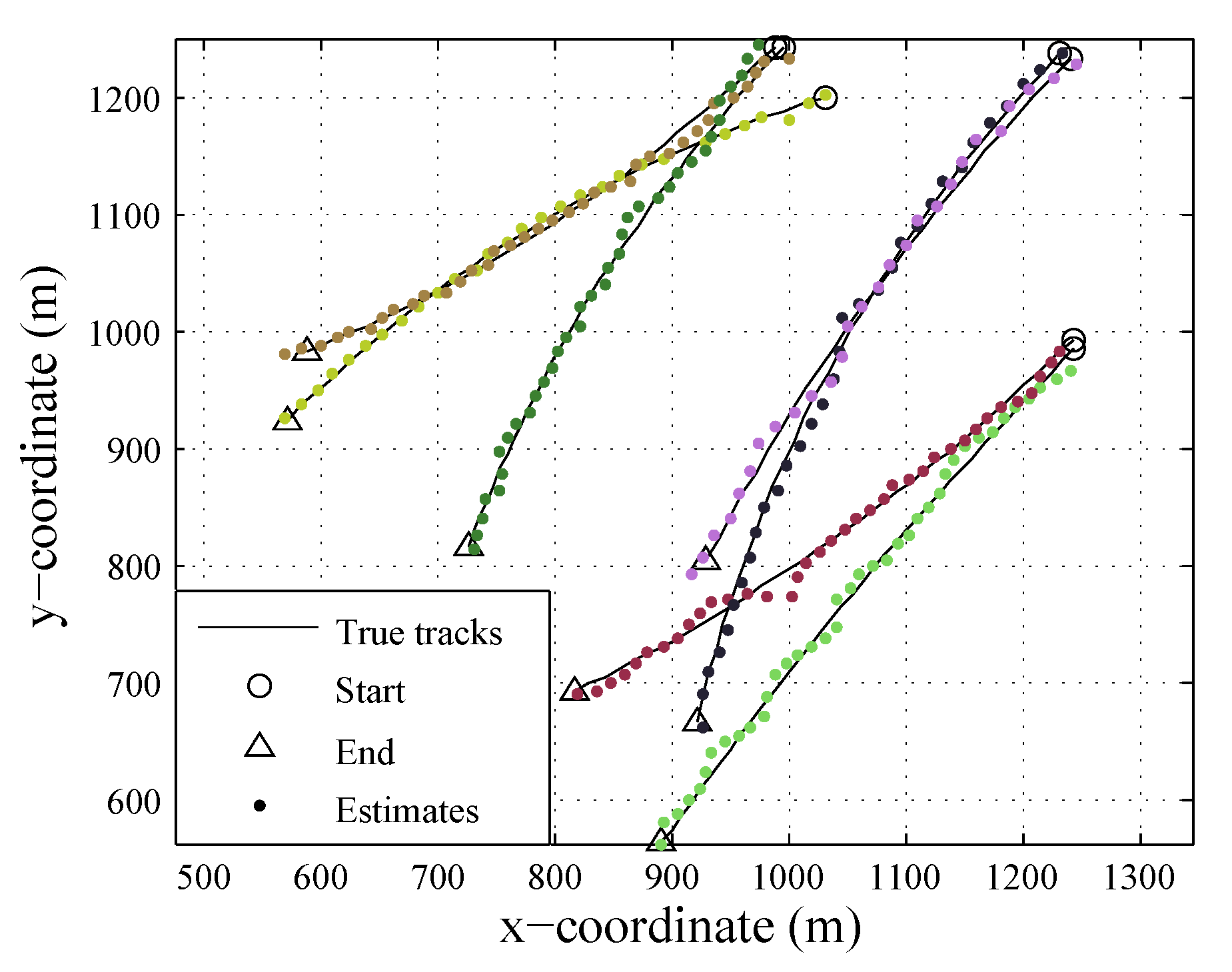
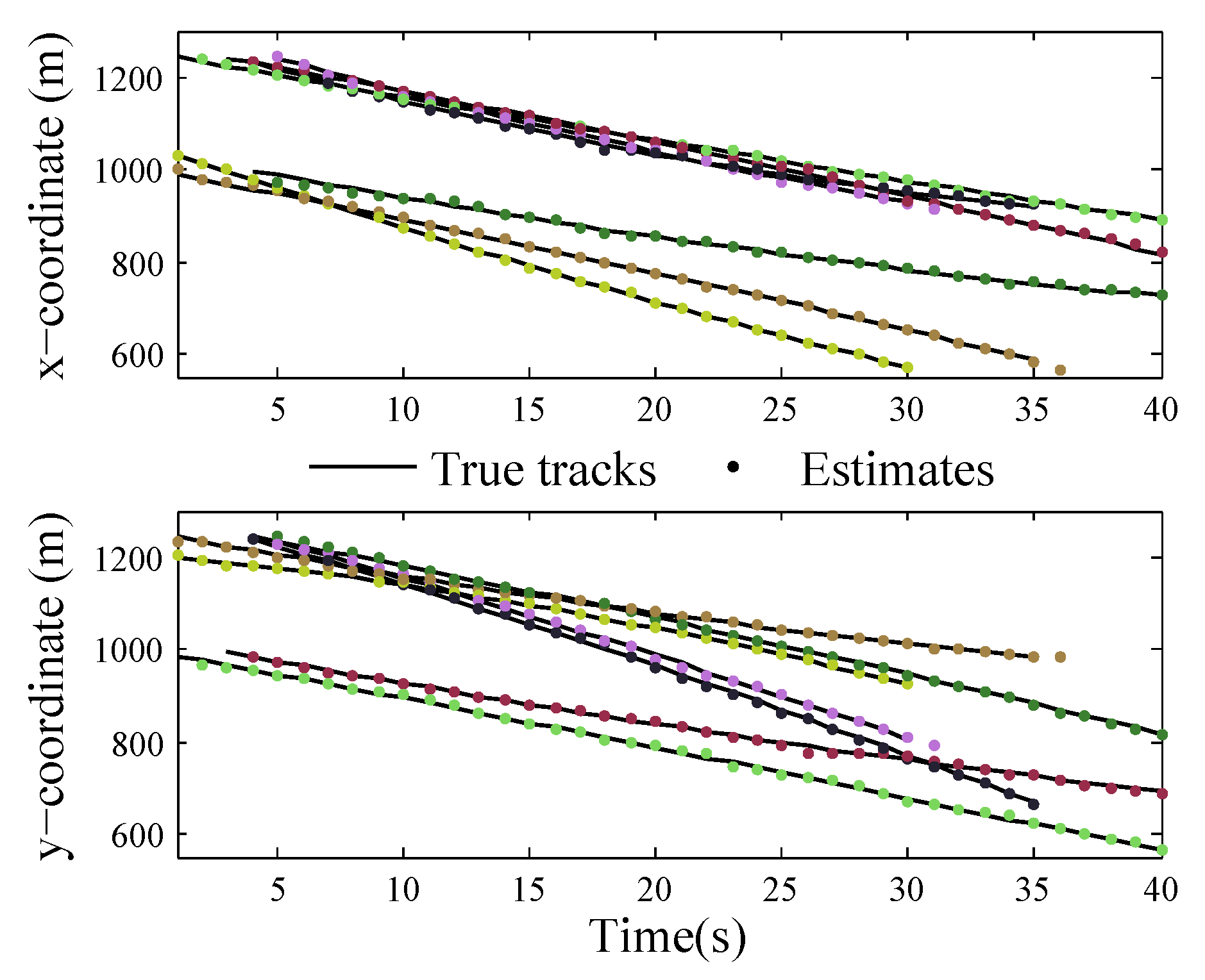
Figure 7, Figure 8, Figure 9, Figure 10 and Figure 11 show the simulation results when SNR is 7 dB. The solid lines in Figure 7 and Figure 8 denote the true positions of the targets. The different trajectories estimated by the S-LMB-GOM filter are denoted by different color dots. It can be seen that there is a small delay in the initiations and terminations of the trajectories and the estimates of each target state and the total cardinality are generally accurate with a small incidence of false tracks in the region of the closely spaced targets. The estimated results of the G-LMB-GOM filter are similar and are not shown.
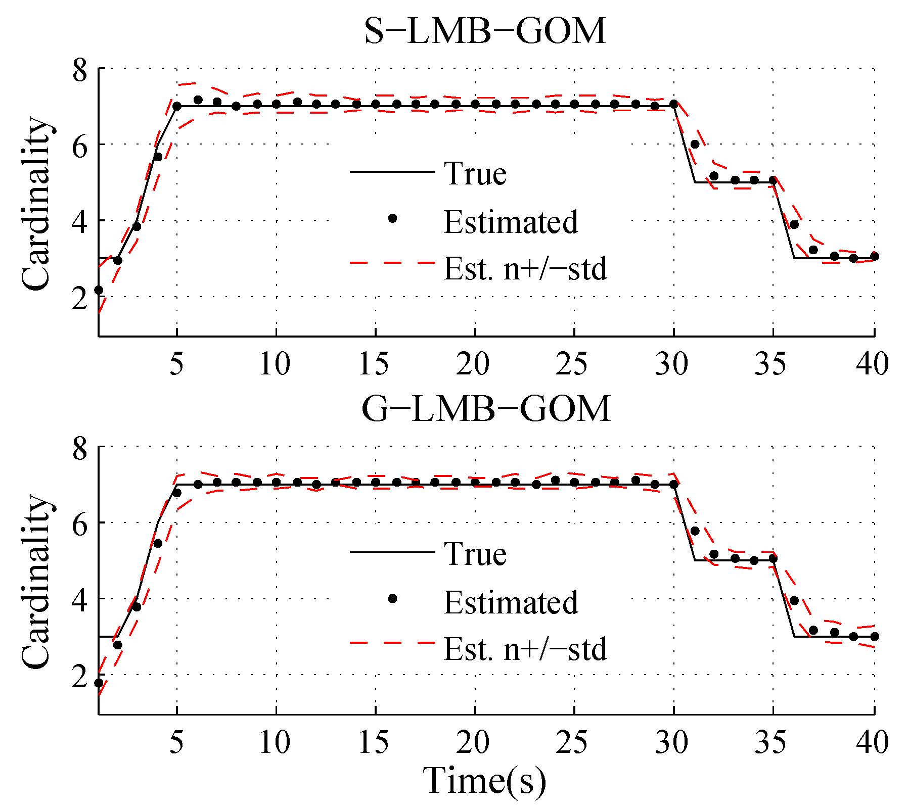
Figure 9 shows the estimated cardinality over 100 Monte Carlo trials. The estimated cardinality mean of two filters both converge to the true cardinality. The estimated cardinality variance of the S-LMB-GOM filter is slightly larger than that of the G-LMB-GOM filter, because the negative effect of the separable likelihood assumption cannot be completely eliminated. The average estimated cardinality variances of two filters are 0.28 and 0.224, respectively.
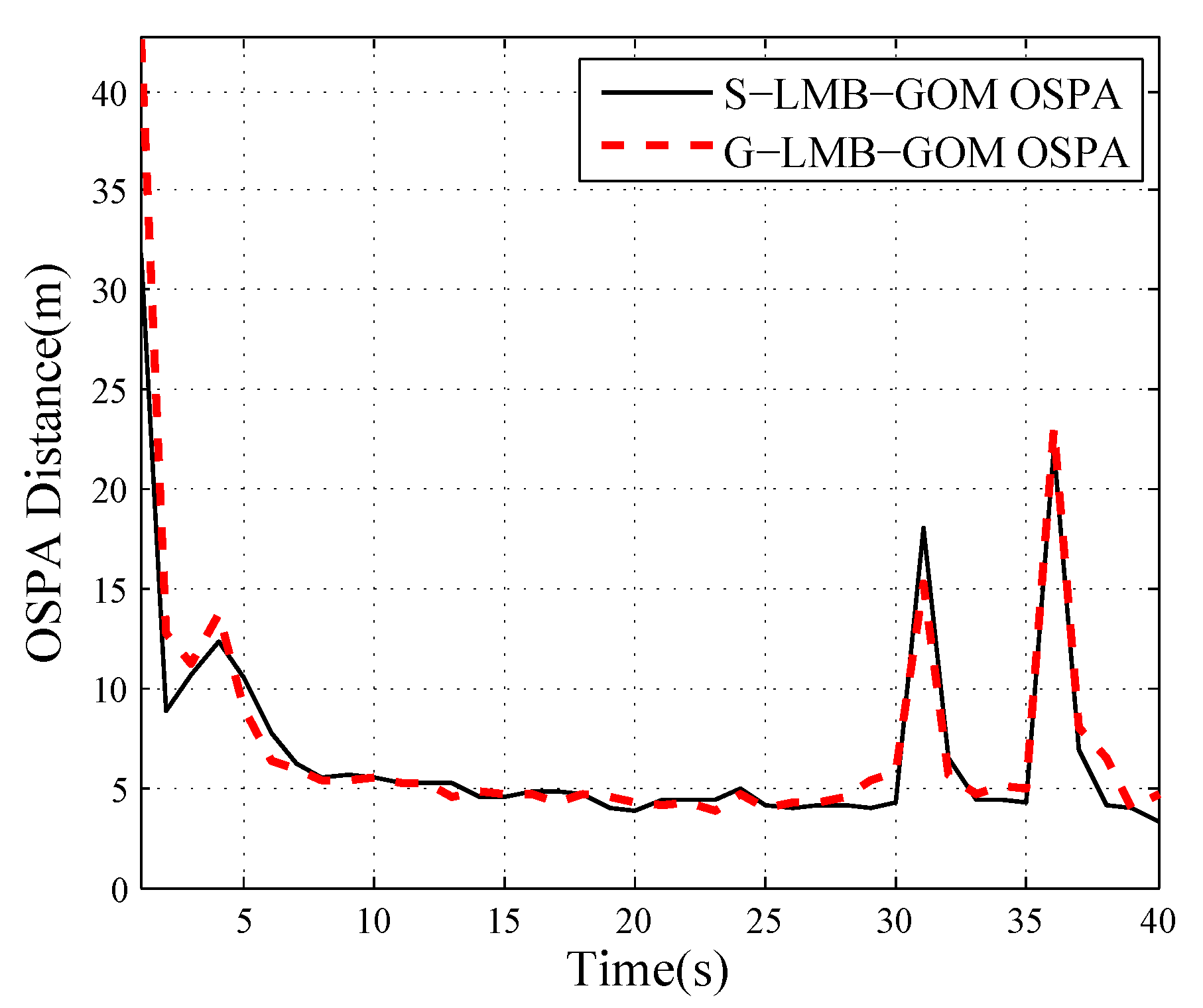
Figure 10 shows the OSPA miss distance for the two filters. The OSPA distance will increase with target births and deaths due to the estimated delay. We also give the average OSPAs of two filters in Table 3. The OSPA in the cardinality errors of the S-LMB-GOM filter is larger than that of the G-LMB-GOM filter, because of the larger cardinality variance for the S-LMB-GOM filter. The OSPA in the localization errors of the S-LMB-GOM filter is less than that of the G-LMB-GOM filter, because of less mutual interference in state estimation for the S-LMB-GOM filter. We can obtain that the total OSPA distance of the S-LMB-GOM filter is slightly less than that of the G-LMB-GOM filter.
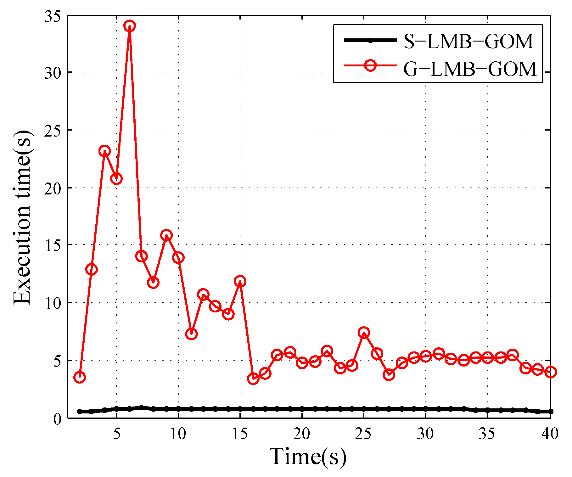
Figure 11 shows the average execution time per frame. The execution time per frame for the S-LMB-GOM filter is less than 1 s. The average time each simulation for the S-LMB-GOM filter is about 29.3 s, while the average time each simulation for the G-LMB-GOM filter is about 323 s. The execution time from the 5th frame to 10th frame is significantly increased for the G-LMB-GOM filter because the hypothesized tracks are relative close and the group processing cannot effectively reduce the computation time.
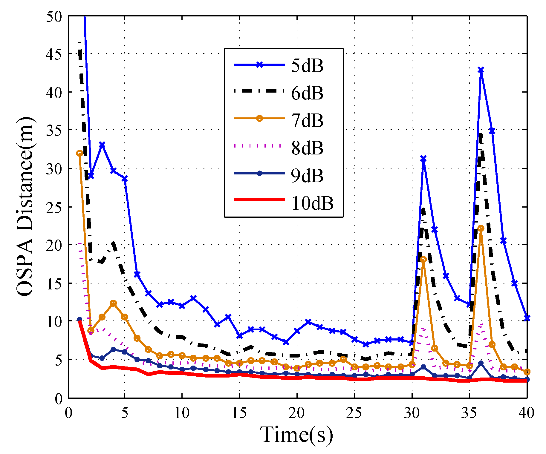
Figure 12 shows the OSPA miss distance at different SNR for the S-LMB-GOM filter. It can be seen that the OSPA distance decreases with increasing SNR.
In general, both filters can track the targets over time and can output the trajectory of each target accurately and stably. From the OSPA miss distances in Table 3, the estimated performances of two filters are similar, but the execution time of the S-LMB-GOM filter is 1 / 11 of the G-LMB-GOM filter. Compared with the G-LMB-GOM filter, our proposed filter can greatly improve the computational efficiency.
Finally, we note that, the trajectories of the targets we studied turn out to be smooth curves (cf. Figure 3, Figure 4 and Figure 7), for which the trajectory fitting approach [31,32] may be applied for better results, either in the manner working by themselves independently or jointly with our proposed filter. To avoid distracting the attention of the reader from our key contribution, we refer the reader to the mentioned works.

5. Conclusions

We analyze the reasons of the cardinality estimate bias for the S-LMB-GOM filter when violating the separable likelihood assumption and then propose a one-to-one correspondence method between measurements and tracks to overcome the problem. In addition, to improve the computational efficiency, we propose an approximate method to calculate point spread function according to its property analysis. We design a TBD simulation with multiple closely spaced targets for radar sensor to evaluate the performance. In comparison with the G-LMB-GOM filter, our proposed algorithm can drastically reduce computational complexity when tracking performance is guaranteed. It should be pointed out that our model is simplified without considering the target amplitude fluctuations in different frames [33,34] so the processing of the real data will be the focus of our future research.

Author Contributions

Methodology, software and writing, R.L.; methodology and review, H.F.; supervision and validation, H.X.

Funding

This research received no external funding.

Conflicts of Interest

The authors declare no conflict of interest.

References

  1. Meyer, F.; Kropfreiter, T.; Williams, J.L.; Lau, R.; Hlawatsch, F.; Braca, P.; Win, M.Z. Message Passing Algorithms for Scalable Multitarget Tracking. Proc. IEEE 2018, 106, 221–259. [Google Scholar] [CrossRef]
  2. Meyer, F.; Win, M.Z. Joint Navigation and Multitarget Tracking in Networks. In Proceedings of the IEEE International Conference on Communications Workshops, Kansas City, MO, USA, 20–24 May 2018; pp. 1–6. [Google Scholar]
  3. Mahler, R.P.S. Statistical Multisource-Multitarget Information Fusion; Artech House, Inc.: Norwood, MA, USA, 2007. [Google Scholar]
  4. Li, T.; Su, J.; Liu, W.; Corchado, J.M. Approximate Gaussian conjugacy: Recursive parametric filtering under nonlinearity, multimodality, uncertainty, and constraint, and beyond. Front. Inf. Technol. Electron. Eng. 2017, 18, 1913–1939. [Google Scholar] [CrossRef]
  5. Mahler, R.P.S. “Statistics 103” for Multitarget Tracking. Sensors 2019, 19, 202. [Google Scholar] [CrossRef] [PubMed]
  6. Mahler, R.P.S. Multitarget Bayes filtering via first-order multitarget moments. IEEE Trans. Aerosp. Electron. Syst. 2004, 39, 1152–1178. [Google Scholar] [CrossRef]
  7. Mahler, R.P.S. PHD filters of higher order in target number. IEEE Trans. Aerosp. Electron. Syst. 2008, 43, 1523–1543. [Google Scholar] [CrossRef]
  8. Vo, B.T.; Vo, B.N.; Cantoni, A. The Cardinality Balanced Multi-Target Multi-Bernoulli Filter and Its Implementations. IEEE Trans. Signal Process. 2009, 57, 409–423. [Google Scholar]
  9. Vo, B.T.; Vo, B.N. Labeled Random Finite Sets and Multi-Object Conjugate Priors. IEEE Trans. Signal Process. 2013, 61, 3460–3475. [Google Scholar] [CrossRef]
  10. Vo, B.N.; Vo, B.T.; Phung, D. Labeled Random Finite Sets and the Bayes Multi-Target Tracking Filter. IEEE Trans. Signal Process. 2014, 62, 6554–6567. [Google Scholar] [CrossRef] [Green Version]
  11. Reuter, S.; Vo, B.T.; Vo, B.N.; Dietmayer, K. The Labeled Multi-Bernoulli Filter. IEEE Trans. Signal Process. 2014, 62, 3246–3260. [Google Scholar]
  12. Mahler, R.P.S. Advances in Statistical Multisource-Multitarget Information Fusion; Artech House: Norwood, MA, USA, 2014. [Google Scholar]
  13. Hoseinnezhad, R.; Vo, B.N.; Vo, B.T.; Suter, D. Visual tracking of numerous targets via multi-Bernoulli filtering of image data. Pattern Recognit. 2012, 45, 3625–3635. [Google Scholar] [CrossRef]
  14. Hoseinnezhad, R.; Vo, B.N.; Vo, B.T. Visual Tracking in Background Subtracted Image Sequences via Multi-Bernoulli Filtering. IEEE Trans. Signal Process. 2013, 61, 392–397. [Google Scholar] [CrossRef]
  15. Nannuru, S.; Coates, M.; Mahler, R. Computationally-Tractable Approximate PHD and CPHD Filters for Superpositional Sensors. IEEE J. Sel. Top. Signal Process. 2013, 7, 410–420. [Google Scholar] [CrossRef]
  16. Nannuru, S.; Coates, M. Particle Filter Implementation of the Multi-Bernoulli Filter for Superpositional Sensors. In Proceedings of the IEEE International Workshop on Computational Advances in Multi-Sensor Adaptive Processing (CAMSAP), St. Martin, France, 15–18 December 2013; pp. 368–371. [Google Scholar]
  17. Mahler, R.P.S. A Fast Labeled Multi-Bernoulli Filter for Superpositional Sensors. In Proceedings of the SPIE, Orlando, FL, USA, 27 April 2018. [Google Scholar]
  18. Beard, M.; Vo, B.T.; Vo, B.N. Bayesian Multi-Target Tracking with Merged Measurements Using Labelled Random Finite Sets. IEEE Trans. Signal Process. 2015, 63, 1433–1447. [Google Scholar] [CrossRef]
  19. Lundquist, C.; Granstrom, K.; Orguner, U. An Extended Target CPHD Filter and a Gamma Gaussian Inverse Wishart Implementation. IEEE J. Sel. Top. Signal Process. 2013, 7, 472–483. [Google Scholar] [CrossRef] [Green Version]
  20. Papi, F.; Vo, B.N.; Vo, B.T.; Fantacci, C.; Beard, M. Generalized Labeled Multi-Bernoulli Approximation of Multi-Object Densities. IEEE Trans. Signal Process. 2015, 63, 5487–5497. [Google Scholar] [CrossRef]
  21. Boers, Y.; Driessen, J.N. Multitarget particle filter track before detect application. Radar Sonar Navig. IEE Proc. 2004, 151, 351–357. [Google Scholar] [CrossRef] [Green Version]
  22. Boers, Y.; Driessen, H.; Torstensson, J.; Trieb, M. Track-before-detect algorithm for tracking extended targets. Radar Sonar Navig. IEE Proc. 2006, 153, 345–351. [Google Scholar] [CrossRef] [Green Version]
  23. Habtemariam, B.K.; Tharmarasa, R.; Kirubarajan, T. PHD filter based track-before-detect for MIMO radars. Signal Process. 2012, 92, 667–678. [Google Scholar] [CrossRef]
  24. Papi, F.; Kyovtorov, V.; Giuliani, R.; Oliveri, F.; Tarchi, D. Bernoulli Filter for Track-Before-Detect using MIMO Radar. IEEE Signal Process. Lett. 2014, 21, 1145–1149. [Google Scholar] [CrossRef]
  25. Papi, F.; Du, Y.K. A Particle Multi-Target Tracker for Superpositional Measurements Using Labeled Random Finite Sets. IEEE Trans. Signal Process. 2015, 63, 4348–4358. [Google Scholar] [CrossRef]
  26. Li, S.; Yi, W.; Hoseinnezhad, R.; Wang, B.; Kong, L. Multiobject Tracking for Generic Observation Model Using Labeled Random Finite Sets. IEEE Trans. Signal Process. 2018, 66, 368–383. [Google Scholar] [CrossRef]
  27. Vo, B.N.; Vo, B.T.; Pham, N.; Suter, D. Joint Detection and Estimation of Multiple Objects From Image Observations. IEEE Trans. Signal Process. 2010, 58, 5129–5141. [Google Scholar] [CrossRef]
  28. Rathnayake, T.; Gostar, A.K.; Hoseinnezhad, R. Labeled Multi-Bernoulli Track-before-Detect for Multi-Target Tracking in Video. In Proceedings of the International Conference on Information Fusion, Washington, DC, USA, 2–5 July 2015; pp. 1353–1358. [Google Scholar]
  29. Blackman, S.S.; Popoli, R. Design and Analysis of Modern Tracking Systems; Artech House: Norwood, MA, USA, 1999. [Google Scholar]
  30. Schuhmacher, D.; Vo, B.T.; Vo, B.N. A consistent metric for performance evaluation of multi-object filters. IEEE Trans. Signal Process. 2008, 56, 3447–3457. [Google Scholar] [CrossRef]
  31. Li, T.; Chen, H.; Sun, S.; Corchado, J.M. Joint Smoothing and Tracking Based on Continuous-Time Target Trajectory Function Fitting. IEEE Trans. Autom. Sci. Eng. 2019, 16, 1476–1483. [Google Scholar] [CrossRef]
  32. Li, T. Single-Road-Constrained Positioning Based on Deterministic Trajectory Geometry. IEEE Comm. Lett. 2019, 23, 80–83. [Google Scholar] [CrossRef]
  33. Rutten, M.G.; Gordon, N.J.; Maskell, S. Recursive track-before-detect with target amplitude fluctuations. Radar Sonar Navig. IEE Proc. 2005, 152, 345–352. [Google Scholar] [CrossRef]
  34. Xia, S.Z.; Liu, H.W. Bayesian track-before-detect algorithm with target amplitude fluctuation based on expectation-maximisation estimation. IET Radar Sonar Navig. 2012, 6, 719–728. [Google Scholar] [CrossRef]
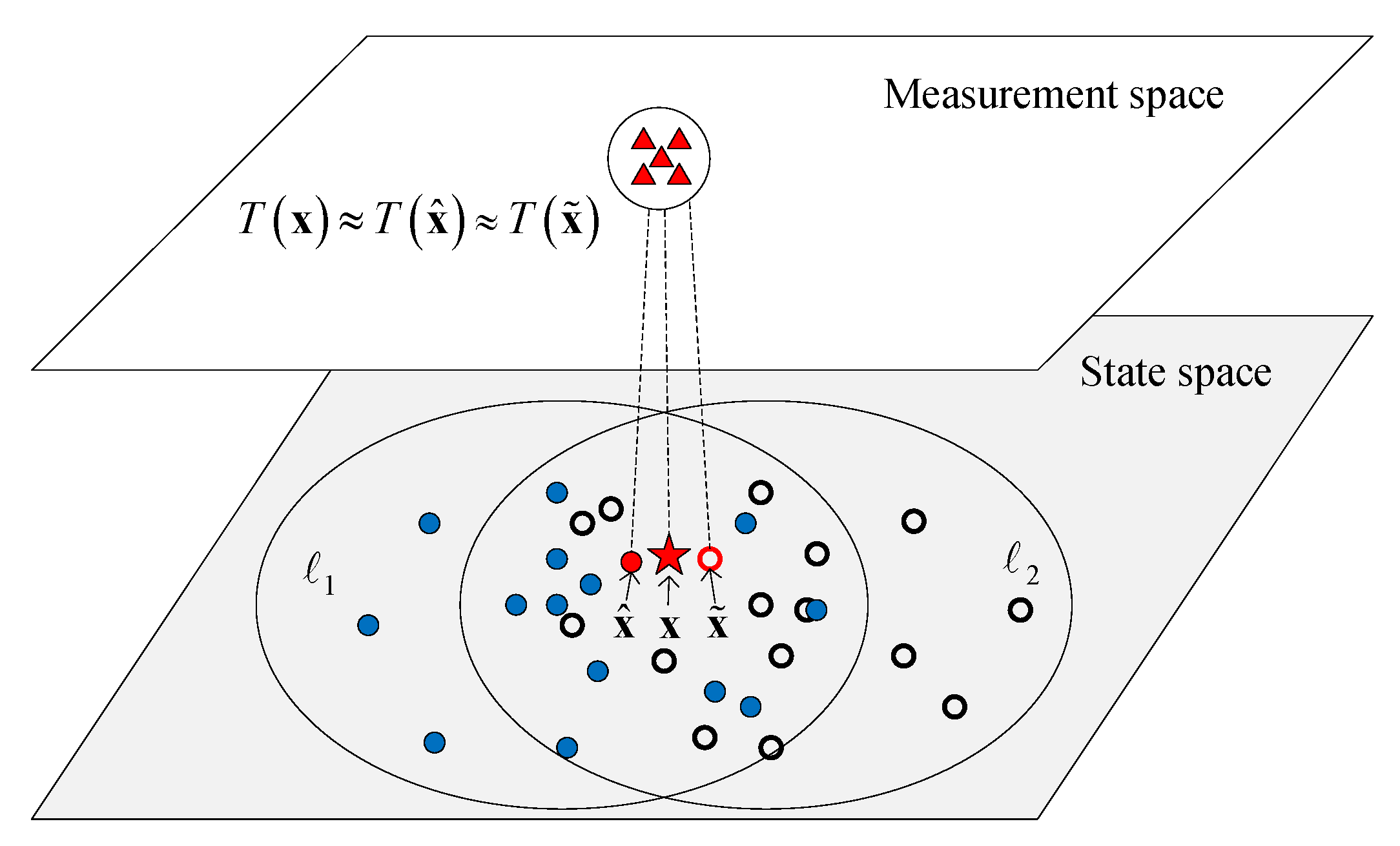
Figure 1. A sketch diagram to show the measurements affected by a target are associated with two tracks. Solid dots denote the particles of track 1 , Hollow dots denote the particles of track 2 and triangles denote the associated measurements of x , x ^ and x ˜ .
Applsci 09 04187 g001
Figure 2. A sketch diagram to show the measurements affected by two targets are associated with two tracks. Solid triangles denote the associated measurements of the target x 1 and the particle x ^ 1 , Hollow triangles denote the associated measurements of the target x 2 and the particle x ^ 2 .
Applsci 09 04187 g002
Figure 3. The true trajectory and estimated trajectory before applying the proposed method.
Applsci 09 04187 g003
Figure 4. The true trajectory and estimated trajectory after applying the proposed method.
Applsci 09 04187 g004
Figure 5. The true cardinality and the estimated cardinality before and after applying the proposed method.
Applsci 09 04187 g005
Figure 6. For simplicity of drawing, C x is a two dimensional matrix and k equals to 3. c t x is the cell of the target x indicated by a orange triangle, c i 0 x is indicated by a hollow red pentagram in the center closest to c t x , C x is the measurement cell set indicated by all pentagrams which is the nearest 3 cells around cell c i 0 x in each dimension and c t x ˜ is indicated by an blue dot which approximates c t x .
Applsci 09 04187 g006
Figure 7. The true and estimated trajectory of a S-LMB-GOM filter.
Applsci 09 04187 g007
Figure 8. The true and estimated trajectory of S-LMB-GOM filter in x and y coordinates.
Applsci 09 04187 g008
Figure 9. The true and estimated cardinality for S-LMB-GOM filter and G-LMB-GOM filter.
Applsci 09 04187 g009
Figure 10. The OSPA distances for S-LMB-GOM filter and G-LMB-GOM filter.
Applsci 09 04187 g010
Figure 11. The execution time per frame for S-LMB-GOM filter and G-LMB-GOM filter.
Applsci 09 04187 g011
Figure 12. The OSPA miss distance at different SNRs for S-LMB-GOM filter.
Applsci 09 04187 g012
Table 1. The confidence level β under different cell number k when c t x = c i 0 x (the corresponded range, azimuth and Doppler cell of the target x is is located in the sampling position) and c t x = c i 0 x + 0.5 c 0 (the corresponded range, azimuth and Doppler cell of the target x is is not located in the sampling position with a offset 0.5 c 0 in each dimension).
Cell Number k β When c t x = c i 0 x β When c t x = c i 0 x + 0.5 c 0
10.06350.0436
30.68820.5794
50.97280.9432
70.99920.9973
90.9999910.999951
Table 2. Some Simulation Parameters.
ParameterSymbolValue
Signal-to-Noise RatioSNR7 dB
Mean of 1st birth track x B 1 [ 1250 , 10 , 1000 , 10 , 0 ] T
Mean of 2st birth track x B 2 [ 1000 , 10 , 1250 , 10 , 0 ] T
Mean of 3st birth track x B 3 [ 1050 , 18 , 1200 , 5 , 0 ] T
Mean of 4st birth track x B 4 [ 1250 , 15 , 1250 , 15 , 0 ] T
Variances of all birth tracksQ d i a g ( 15 , 2 , 15 , 2 , 2 π / 180 ) 2
Range ResolutionR5 m
Azimuth ResolutionB π / 180 rad
Doppler ResolutionD1 m/s
Time Sampling Interval T s 1 s
Table 3. Average OSPA distances for the S-LMB-GOM filter and the G-LMB-GOM filter.
MethodLocalizationCardinalityTotal
Component (m)Component (m)OSPA (m)
S-LMB4.12.957.05
G-LMB4.482.817.29