SOC Estimation with an Adaptive Unscented Kalman Filter Based on Model Parameter Optimization

Featured Application

The method of the research can be applied to the estimation of the remaining battery charge of electric vehicles.

Abstract

State of charge (SOC) estimation is generally acknowledged to be one of the most important functions of the battery management system (BMS) and is thus widely studied in academia and industry. Based on an accurate SOC estimation, the BMS can optimize energy efficiency and protect the battery from being over-charged or over-discharged. The accurate online estimation of the SOC is studied in this paper. First, it is proved that the second-order resistance capacitance (RC) model is the most suitable equivalent circuit model compared with the Thevenin and multi-order models. The second-order RC equivalent circuit model is established, and the model parameters are identified. Second, the reasonable optimization of model parameters is studied, and a reasonable optimization method is proposed to improve the accuracy of SOC estimation. Finally, the SOC is estimated online based on the adaptive unscented Kalman filter (AUKF) with optimized model parameters, and the results are compared with the results of an estimation based on pre-optimization model parameters. Simulation experiments show that, without affecting the convergence of the initial error of the AUKF, the model after parameter optimization has a higher online SOC estimation accuracy.

1. Introduction

The power battery State of charge (SOC) is generally defined as the ratio between the available capacity and the reference capacity. An accurate SOC estimation is an important basis for the formulation of an optimal energy management strategy for the whole vehicle control system of an electric vehicle (EV). It is of great significance for extending the life of the battery pack and improving the safety of the battery system [1,2]. Due to the nonlinear nature of the power battery, the SOC cannot be directly acquired by sensors; rather, it must be estimated by measuring physical quantities, such as the battery voltage, operating current, and internal resistance of the battery, and by using certain mathematical methods [3,4].

Commonly used estimation methods include the open-circuit voltage method, the ampere-hour integration method, the neural network method and the Kalman filter method [5,6,7,8,9]. The open-circuit voltage (OCV) can represent the discharge capacity of a lithium battery in its current state. It has a good linear relationship with the SOC when the SOC is greater than 0.1. The OCV cannot be directly measured during the working state of the battery; it can only be approximated when the battery is not working. Therefore, this method is only applicable to EVs that are parked, and the OCV method is used to provide an initial value of the SOC for other estimation methods. The ampere-hour (Ah) integral method is a relatively common, simple and reliable method for estimating the SOC. When the discharge current is positive and the charging current is negative, the calculation formula can be expressed as:

$$SO{C}_t=SO{C}_0-\frac{1}{C_N}{\displaystyle {\int }_0^t\eta idt}$$

(1)

where SOC₀ is the initial SOC value, C_N is the maximum available capacity of the battery, which is almost invariant if the time scale is small and battery ageing is accordingly ignored [8], and η is the coulomb efficiency. The ampere-hour integral method has the advantages of low cost and convenient measurement. However, there are several problems in the application of this method in EVs: (1) Other methods are needed to obtain the initial value of the SOC. (2) The accuracy of the current measurement has a decisive influence on the accuracy of the SOC estimation. (3) The cumulative error of the integration process cannot be eliminated, and if the charging or discharging time is too long during one calculation, cumulative errors can cause estimates to be unreliable.

A neural network (NN) is an intelligent mathematical tool [10,11]. A NN has the adaptability and self-learning skills to demonstrate a complex nonlinear model. NNs use trained data to estimate the SOC without knowing any information about the internal structure of the battery and the initial SOC. Theoretically, the nonlinear characteristics of the power battery can be better mapped by a NN. The advantage of this method is that it is capable of working in nonlinear battery conditions while the battery is charging/discharging. Nevertheless, the algorithm needs to store a large amount of data for training, which not only requires large memory storage but also overloads the entire system.

The Kalman filter method [12,13,14] is the current research hotspot for SOC estimation. The core idea of the Kalman filter is the optimal estimate in the sense of minimum variance, including the two stages of prediction and updating. In the prediction stage, the filter applies the value of the previous state to estimate the current state, and in the updating stage, the filter optimizes the predicted value in the prediction stage by using the observed value in the current state to obtain a more accurate estimate of the current state. It should be noted that the basic Kalman filter is mainly applied to linear systems. However, the estimation of the SOC is related to many factors, such as charge and discharge current, and cut-off voltage, and the influence of these factors on the SOC is nonlinear. For this reason, some people have used the extended Kalman filter (EKF) to estimate the battery SOC. Although some achievements have been made, there is a linearization error in actual use, and the Jacobian matrix is difficult to estimate. In recent years, a novel derivative Kalman filter algorithm, the unscented Kalman filter (UKF), has emerged to realize nonlinear filtering. The UKF directly uses nonlinear unscented transform techniques without the need for Taylor approximations of nonlinear equations. This process allows the mean and variance of the state of the nonlinear system to propagate directly according to the nonlinear mapping, thereby achieving a higher estimation accuracy.

In the traditional UKF algorithm [15,16,17,18,19], the covariance is a constant and cannot satisfy the real-time dynamic characteristics of the noise, which has a certain impact on the accuracy [20,21]. To eliminate this effect, the traditional UKF algorithm is improved by updating the covariance in real-time, which thus improves the accuracy of the UKF in this paper. This type of algorithm is called the adaptive unscented Kalman filter (AUKF) algorithm. On this basis, a reasonable optimization of the model parameters is studied, and a reasonable optimization method is proposed to further improve the accuracy of SOC estimation.

The structure of this paper is arranged as follows. In Section 1, the most commonly used methods for SOC estimation are introduced, and the proposed method of this paper is briefly described. In Section 2, the battery model is established, the model parameters are identified, and the model accuracy is verified. In Section 3, the AUKF based on a second-order resistance capacitance (RC) equivalent circuit model is presented. In Section 4, the basis and method of the reasonable optimization of the model parameters are put forward. In Section 5, the accuracy and initial error convergence of the AUKF before and after model parameter optimization are compared by simulation experiments, and the advantages of the proposed method are demonstrated. Finally, in Section 6, the research results of this paper are summarized, and future research directions are provided.

2. Establishment of Battery Model and Parameter Identification

The open-circuit voltage and internal resistance are the most basic components of an equivalent circuit model. All equivalent circuit models add other components on the basis of these two components to improve the model accuracy. Typical equivalent circuit models of lithium-ion batteries include the Rint model, the Thevenin model, the PNGV (Partnership for a New Generation of Vehicles) model and the multi-order RC loop model [22,23,24,25]. For the complicated polarization characteristics of a battery, some studies deduce and suggest that the models with more parallel RC networks connected in series should have a much higher accuracy; however, at the same time, memory is consumed, waste calculations are performed and bad real-time applications are caused.

2.1. Establishment of Lithium-Ion Battery Model

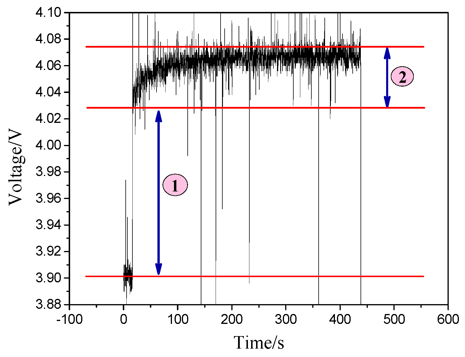
The measured terminal voltage response curve of the Sanyo lithium battery with a rated capacity of 2.6 AH at a certain state (SOC = 0.9 with a constant current discharge of 260 mAh at 0.5 C) at the end of discharge is shown in Figure 1.

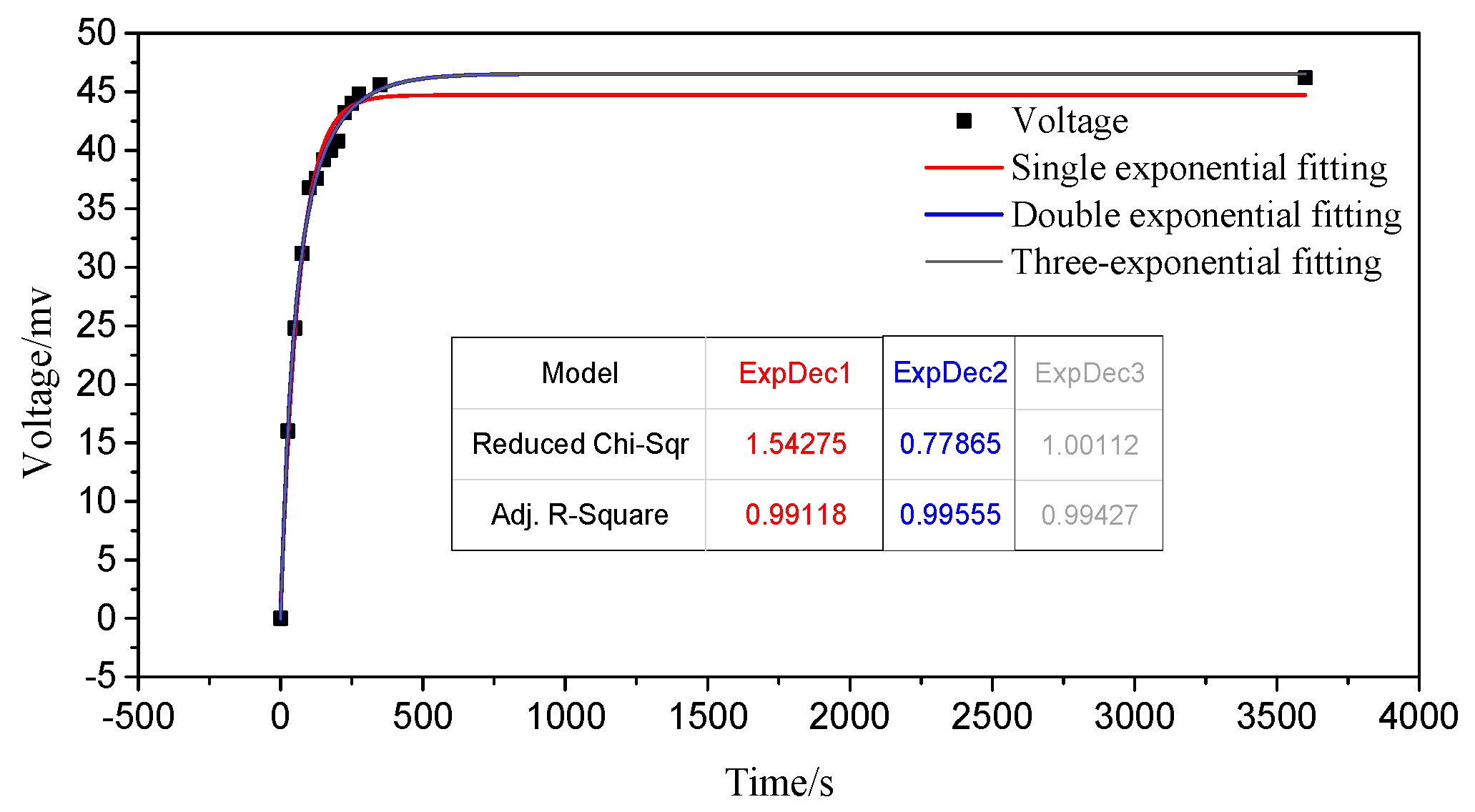
The polarization effect of a lithium battery is usually expressed equivalently by an RC loop and is equivalent to the first-order zero input response after the battery is discharged. Its terminal voltage can be expressed as an exponential term ($IR{e}^{\frac{-t}{\tau }}$). Region 2 in Figure 1 is the disappearance process of the polarization effect. Exponential curves are used to fit the single index, double index and triple index coefficients of region 2, and the fitting results are shown in Figure 2.

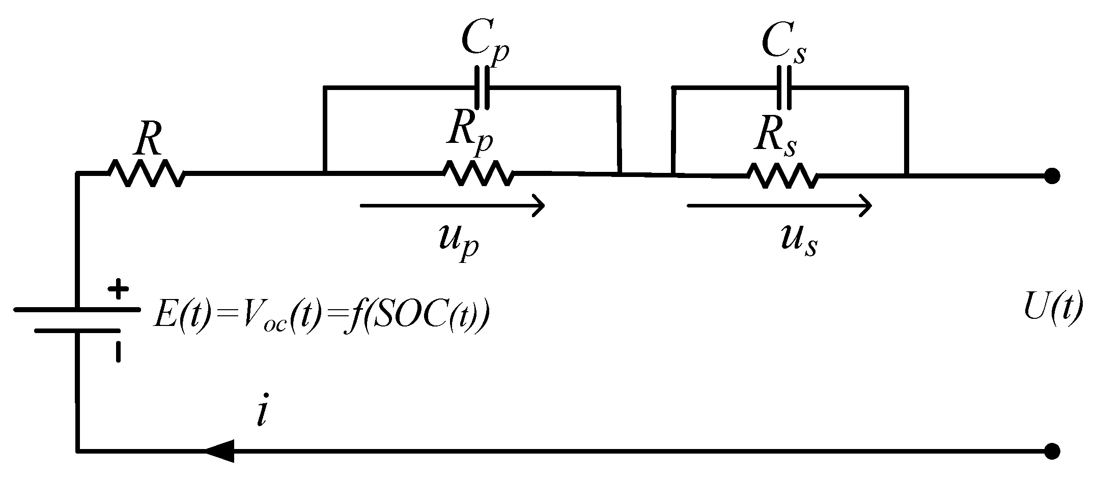
It can be seen from Figure 2 that the reduced chi-squared statistics of the double and triple exponential fittings are smaller than that of the single exponential fitting. That is, the random error effect of the double and triple exponential fittings are smaller than that of the single exponential fitting. At the same time, the correction decision coefficient of the double and triple exponential fittings is larger than that of the single exponential fitting and is closer to 1, and the fitting effect is better. Therefore, the double and triple exponential fittings can more accurately reflect the polarization effect of the battery. By comparing the results of the double and triple exponential fittings, the sum of the squares of the residuals of the double exponential fitting is less than that of the triple exponential fitting, and the correction decision coefficient of the double exponential fitting is also closer to 1 than that of the triple exponential fitting. The results show that the double exponential fitting effect is better than the triple exponential fitting effect. The reason for this fitting result is that although the third-order RC loop can theoretically better reflect the dynamic characteristics of the battery, the third-order RC loop has one more RC loop than the second-order RC loop, which means that the third-order RC loop has two more unknowns than the second-order RC loop in the process of data fitting by computer. Therefore, the fitting effect of the third-order RC loop is not as good as that of the second-order RC loop, and it is proved that the second-order RC model is better than the others for a lithium battery. On this basis, considered comprehensively, the second-order RC equivalent circuit model, as shown in Figure 3, is adopted in this paper.

The model consists of three parts:

Voltage source: V_oc represents the open circuit voltage of the power battery. In this paper, the influences of temperature and state of health (SOH) on the OCV are not considered, and the functional relationship between V_oc and the battery SOC is studied under the same temperature and SOH conditions. Additionally, the effect of corrosion on the battery is neglected because the focus of this paper is on the equivalent circuit model.

Ohmic resistance: R is used to represent the internal resistance of the battery, which can be determined by the sudden change in voltage after the end of discharge, as shown in region 1 of Figure 1.

RC loop circuit: Two links of a resistor and a capacitor are superposed to simulate battery polarization, which is used to simulate the process of voltage stabilization after discharge. Region 2 of Figure 1 shows the change in voltage influenced by the RC loop circuit.

As shown in Figure 3, the functional relationship of the equivalent circuit model is as follows:

$$\{\begin{array}{c}E\left(t\right)=iR+u_s+u_p+U\left(t\right)=F\left(SOC\left(t\right)\right)\\ i=\frac{u_s}{R_s}+C_s\frac{d{u}_s}{dt}\\ i=\frac{u_p}{R_p}+C_p\frac{d{u}_p}{dt}\end{array}$$

(2)

For the discretization of Equation (2), the state equation is solved as:

$$\left[\begin{array}{c}{u}_{s,k}\\ u_{p,k}\end{array}\right]=\left[\begin{array}{cc}{a}_s& 0\\ 0& a_p\end{array}\right]\left[\begin{array}{c}{u}_{s,k-1}\\ u_{p,k-1}\end{array}\right]+\left[\begin{array}{c}{b}_s\\ b_p\end{array}\right]I_{k-1}+\left[\begin{array}{c}{w}_3\left(k\right)\\ w_5\left(k\right)\end{array}\right]$$

(3)

$$U_k=E_k-I_{k}R-U_{s,k}-U_{p,k}+v\left(k\right)=F\left(SO{C}_k\right)-I_{k}R-U_{s,k}-U_{p,k}+v\left(k\right)$$

(4)

of which:

$$\{\begin{array}{c}{a}_s=e^{\frac{-T}{R_s{C}_s}}, b_s=R_s-R_s{e}^{\frac{-T}{R_s{C}_s}} \\ a_p=e^{\frac{-T}{R_p{C}_p}}, b_p=R_p-R_p{e}^{\frac{-T}{R_p{C}_p}}\end{array}$$

(5)

2.2. Identification and Verification of Battery Model Parameters

In the process of establishing the battery model, it is necessary to use the approximate linear relationship between the OCV and the SOC. In this section, based on the OCV–SOC relationship curve, the parameters of the second-order RC model are identified, and then the accuracy of the model is verified.

2.2.1. Obtaining the OCV–SOC Relationship Curve

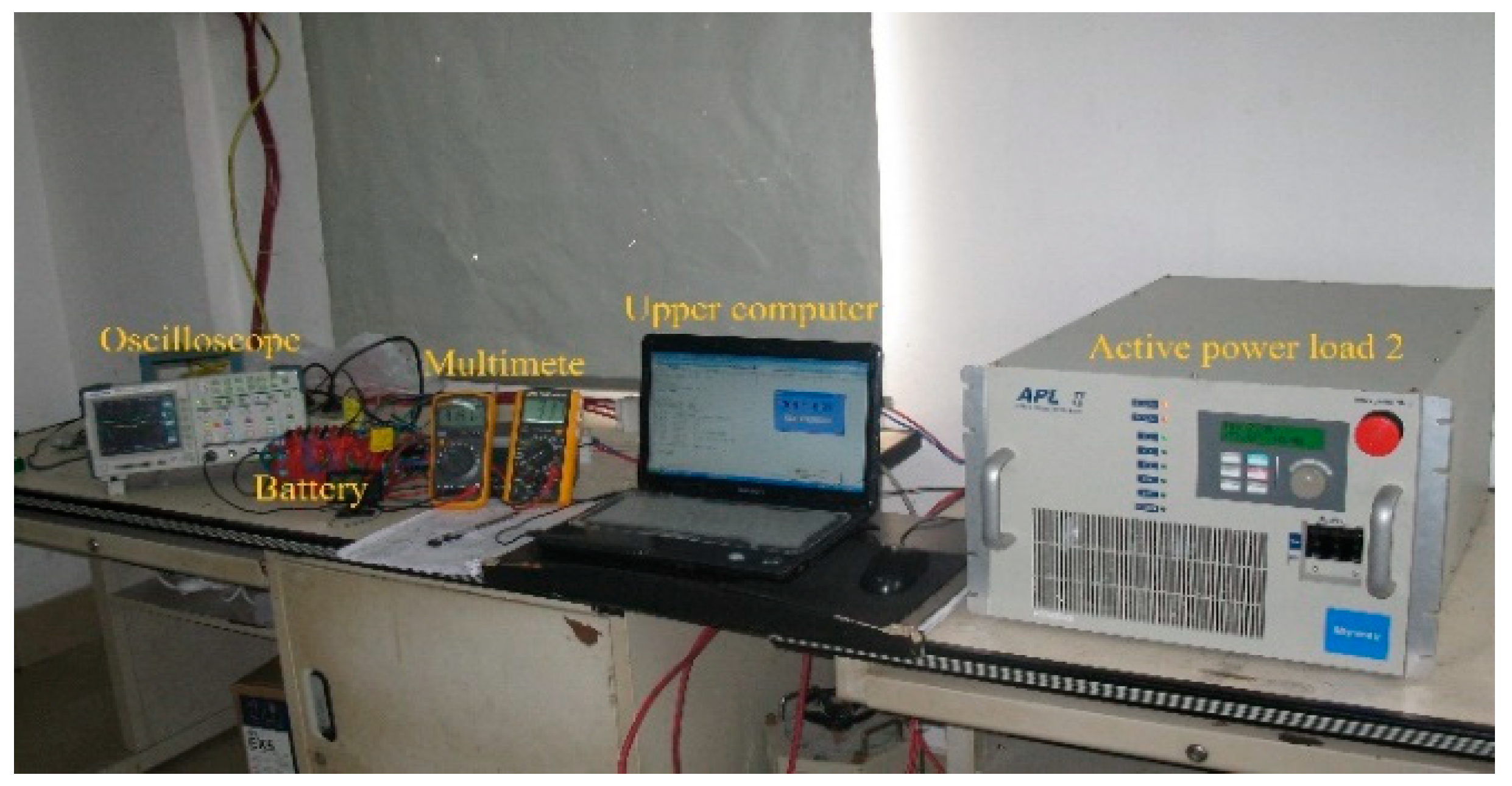
The OCV–SOC curve was obtained from a 18,650 cylindrical lithium-ion battery manufactured by the Sanyo Corporation of Japan with a rated capacity of 2.6 Ah and a rated voltage of 3.7 V, as before. Charge and discharge experiments were carried out on the new battery at a constant temperature. The battery test platform is shown in Figure 4.

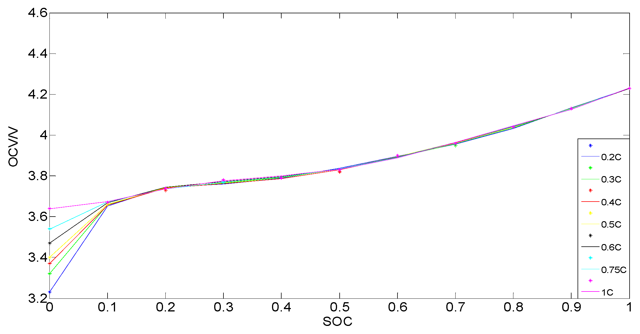
The OCV–SOC curves are calibrated under constant current and constant capacity intermittent discharge conditions of 0.2 C, 0.3 C, 0.4 C, 0.5 C, 0.6 C, 0.75 C and 1 C. The specific calibration process of each group is as follows [3]:

• First, the battery is charged with a constant current (0.2 C), and then the battery is charged with a constant voltage (cut-off voltage of 4.25 V). After charging is completed, the battery is left for one hour to eliminate the polarization effect;
• The battery is discharged with a constant current and a constant capacity (1/10 of the total capacity, 260 mAh);
• After the discharge is complete, the battery is left for one hour, and then the open circuit voltage is measured;
• Repeat steps 2 and 3 until the battery is completely discharged.

The calibration experiment results are shown in Figure 5. When the SOC is greater than 10%, the curves almost coincide. This shows that the OCV–SOC curves corresponding to different discharge rates are approximate under the same temperature (25 °C) and health conditions. In this paper, the OCV–SOC curve under the condition of 0.2 C constant current intermittent discharge is selected as the reference curve.

Using MATLAB to fit the polynomial coefficients, the approximate linear relationship between the OCV and the SOC can be obtained, as shown in Equation (6):

$$Voc=a1\times SO{C}^6+a2\times SO{C}^5+a3\times SO{C}^4+a4\times SO{C}^3+a5\times SO{C}^2+a6\times SOC+a7$$

(6)

where a₁ = −34.72, a₂ = 120.7, a₃ = −165.9, a₄ = 114.5, a₅ = −40.9, a₆ = 7.31, and a₇ = 3.231.

2.2.2. Model Parameter Identification

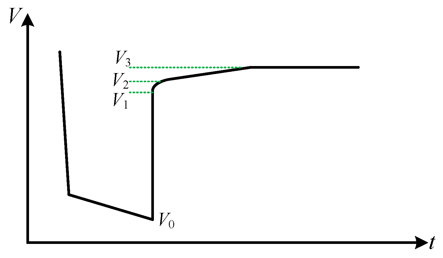
Figure 6 is a schematic diagram of the terminal voltage response curve at the end of lithium battery discharge.

$\left(V_1-V_0\right)$ is the process in which the voltage drop generated on the ohmic resistance inside the battery disappears at the end of discharge. Thus, the ohmic resistance of the battery can be obtained as $R=\frac{V_1-V_0}{I}$. The battery model adopted in this paper simulates the polarization process of the battery by superposing two RC links. An RC parallel circuit with a small time constant is used to simulate the process of rapid voltage change $\left(V_2-V_1\right)$ when the current of the battery changes abruptly. An RC parallel circuit with a large time constant is used to simulate the process of slow voltage change $\left(V_3-V_2\right)$ when the current of the battery changes abruptly.

The battery is assumed to discharge for a period of time during $\left(t_0-t_r\right)$ and then stay in a resting state for the remaining time. Here, $t_0$, $t_d$, and $t_r$ are the discharge start time, the discharge stop time and the static stop time, respectively. In this process, the RC network voltages are:

$$U_s=\{\begin{array}{c}{R}_{s}i\left(t\right)\left[1-e^{\frac{-\left(t-t_0\right)}{{\tau }_s}}\right] t_0<t\le t_d\\ U_s\left(t_d\right)e^{\frac{-\left(t-t_d\right)}{{\tau }_s}} t_d<t<t_r\end{array}$$

(7)

$$U_p=\{\begin{array}{c}{R}_{p}i\left(t\right)\left[1-e^{\frac{-\left(t-t_0\right)}{{\tau }_p}}\right] t_0<t\le t_d\\ U_p\left(t_d\right)e^{\frac{-\left(t-t_d\right)}{{\tau }_p}} t_d<t<t_r\end{array}$$

(8)

Let ${\tau }_s=R_s{C}_s\mathrm{and}{\tau }_p=R_p{C}_p$ be the time constants of the two parallel circuits. The voltage change $\left(V_3-V_1\right)$ is caused by the disappearance of the polarization effect of the battery. In this process, the battery voltage output is $V=E-I{R}_s{e}^{\frac{-t}{{\tau }_s}}-I{R}_p{e}^{\frac{-t}{{\tau }_p}}$, which can be simply written as $V=E-a{e}^{-ct}-b{e}^{-dt}$. This form can be used to fit the coefficients of the double exponential terms with MATLAB. After calculating a, b, c and d, according to $R_s=\raisebox{1ex}{$a$}\!\left/ \!\raisebox{-1ex}{$I$}\right.$, $R_p=\raisebox{1ex}{$b$}\!\left/ \!\raisebox{-1ex}{$I$}\right.$, $C_s=\raisebox{1ex}{$1$}\!\left/ \!\raisebox{-1ex}{$R_{s}c$}\right.$, and $C_p=\raisebox{1ex}{$1$}\!\left/ \!\raisebox{-1ex}{$R_{p}d$}\right.$, the values of $R_s,R_p,C_s,\mathrm{and}{C}_p$ can be identified.

2.2.3. Model Accuracy Verification

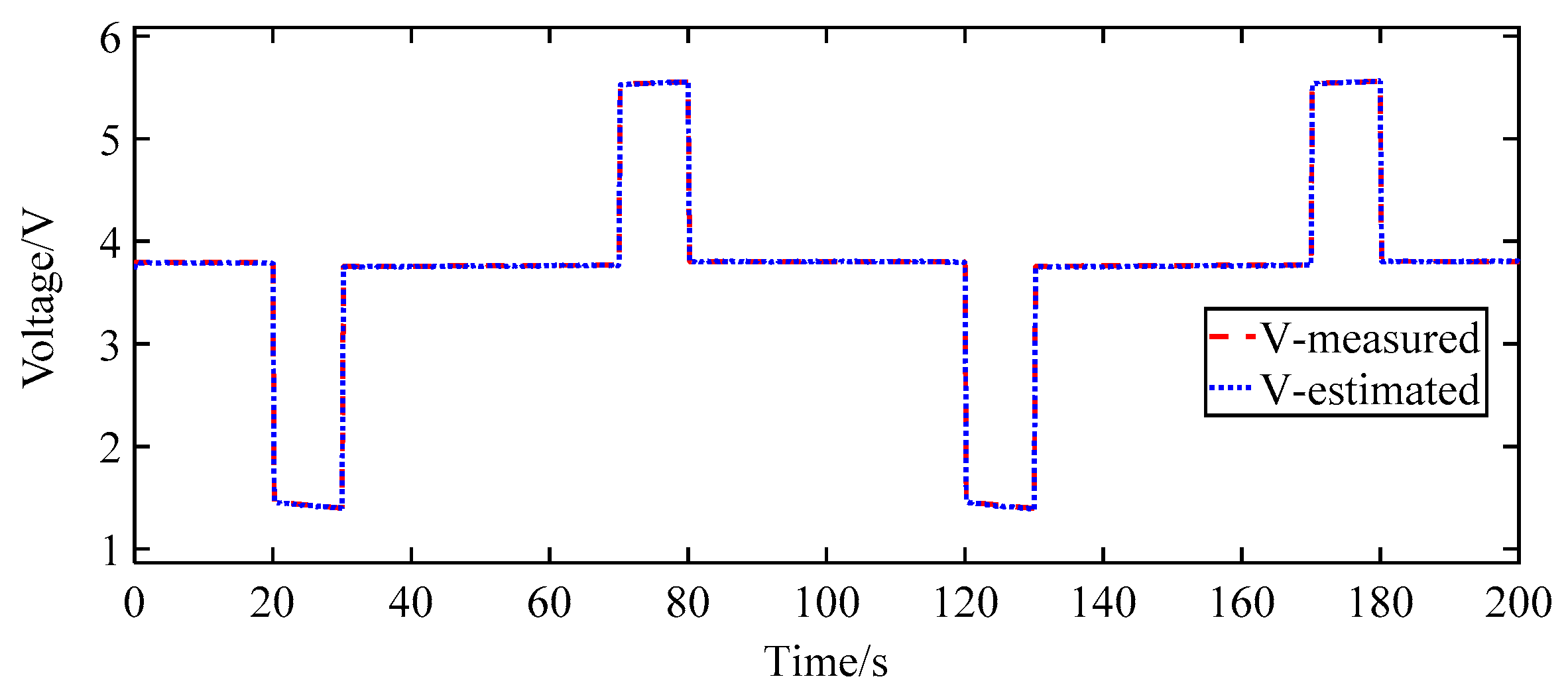
After the model parameters have been identified, the accuracy of the model needs to be verified to determine whether the model parameters can be used for SOC estimation and parameter optimization in this paper. The precision of the model is verified by referring to the hybrid pulse power characterization (HPPC) experiment [26]. The simulated initial SOC is set to 0.5. 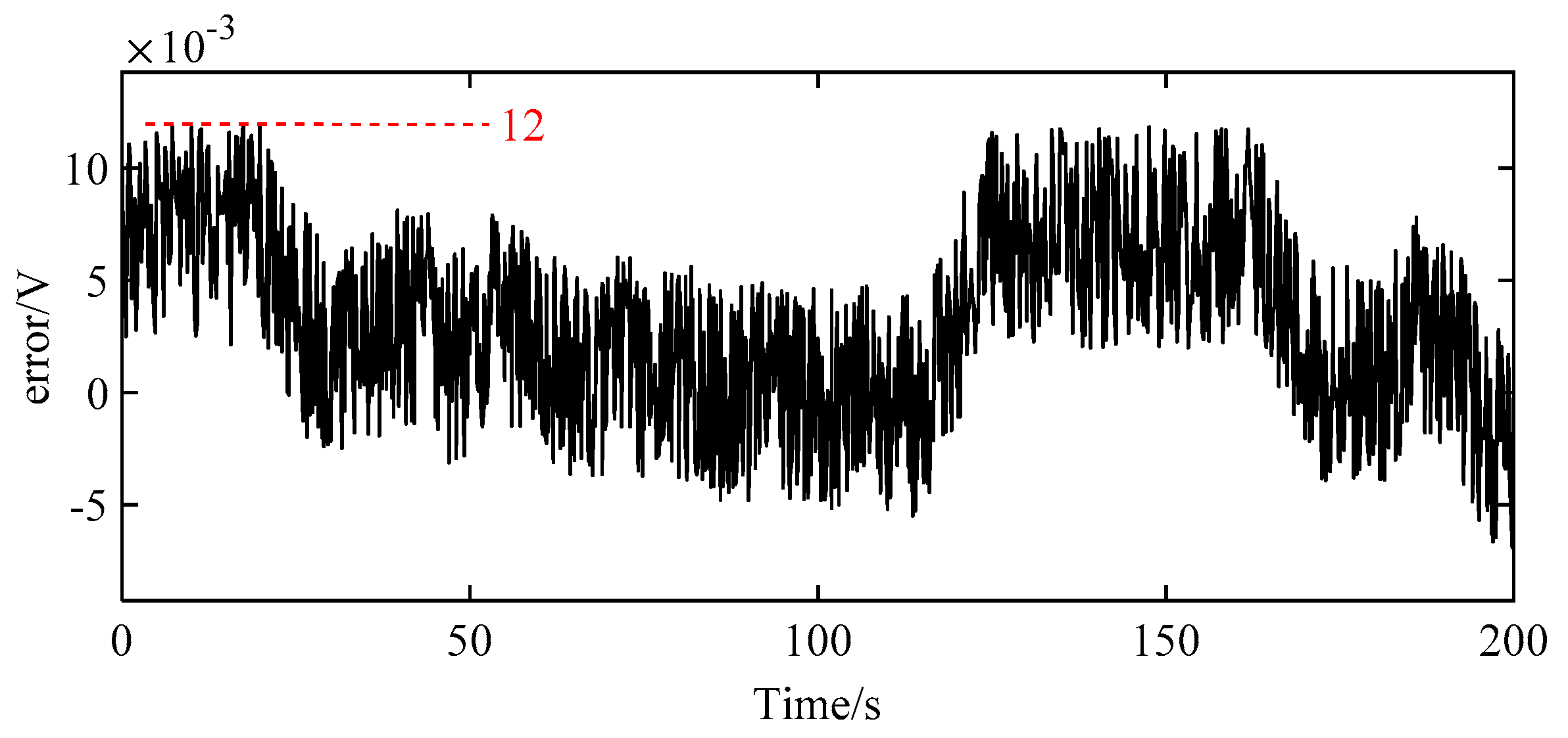The comparison between the experimentally measured voltage and the model simulation output voltage is shown in Figure 7. To better distinguish the difference, the error is presented in Figure 8.

As seen from Figure 7 and Figure 8, when the output voltage of the battery changes due to abrupt current changes, the output voltage of the simulation model can better track the measured voltage. The maximum error is 12 mV, which indicates that the model parameters can be used for the online SOC estimation of the Kalman filter and reasonable parameter optimization.

3. The AUKF Based on the Second-Order RC Equivalent Circuit Model

Based on the equivalent circuit model, the corresponding SOC estimation algorithm can be established. A power lithium battery is a typical nonlinear system. The nonlinear system is governed by the equations of state, and the observation equations are shown in Equation (9).

$$\{\begin{array}{l}{\mathrm{x}}_k=f\left(x_{k-1},u_{k-1}\right)+{\omega }_{k-1}\\ y_k=h(x_k,u_k)+v_k\end{array}$$

(9)

where the random variables w_k and v_k represent the process and measurement noise, respectively. For the UKF, the iteration equation is based on a certain set of sample points, which are chosen to make their mean value and variance consistent with the mean value and variance of the state variables. Then, these points will recycle the equation of the discrete-time process model to produce a set of predicted points. After, the mean value and the variance of the predicted points will be calculated to modify the results, and the mean value and the variance will be estimated. Before the UKF recursion, the state variables must be modified in a superposition of the process noise and the measurement noise of the original states. The SOC of the lithium battery pack can be calculated using the ampere-hour integral method:

$$SOC(t)=SOC(t^{\prime })-\frac{1}{C_N}{\displaystyle {\int }_{t^{\prime }}^t\eta idt}$$

(10)

In Equation (10), $\eta =\frac{k_i{k}_t}{k_c}$, where k_i is the compensation coefficient of the charge and discharge rate, k_t is the temperature compensation coefficient, k_c is the cycle compensation coefficient, and C_N is the actual available battery capacity. From the equivalent circuit model shown in Figure 3, the lithium battery equation of state can be obtained from Equations (2) and (10):

$$\left[\begin{array}{l}SO{C}_k\\ u_{s,k}\\ u_{p,k}\end{array}\right]=\left[\begin{array}{ccc}1& 0& 0\\ 0& a_s& 0\\ 0& 0& a_p\end{array}\right]\left[\begin{array}{l}SO{C}_{k-1}\\ u_{s,k-1}\\ u_{p,k-1}\end{array}\right]+\left[\begin{array}{c}\frac{\eta T}{C_N}\\ b_s\\ b_p\end{array}\right]I_{k-1}+\left[\begin{array}{l}{\omega }_1(k)\\ {\omega }_3(k)\\ {\omega }_5(k)\end{array}\right]$$

(11)

$$\begin{array}{l}{U}_k=E_k-I_{k}R-U_{s,k}-U_{p,k}+v(k)\\ =F(SO{C}_k)-I_{k}R-U_{s,k}-U_{p,k}+v(k)\end{array}$$

(12)

where the values of each coefficient are shown in Equation (5). For the circuit model shown in Equations (11) and (12):

$$X_k={[x_k^T,{\omega }_k^T,v_k^T]}^T={[SO{C}_k,u_{s,k},u_{p,k},{\omega }_{soc,k},{\omega }_{s,k},{\omega }_{p,k},v_k]}^T$$

(13)

To facilitate the distinction, we can take $x_k=\left[SO{C}_k,U_{s,k},U_{p,k}\right]$ as the initial state of the system, y_k as the raw output (its corresponding symbol is U_k in the circuit model of the lithium battery), and u_k as the control variable (its corresponding symbol is I_k), and we can make $\mathsf{\Psi }=\left[y_1,y_2,\cdots ,y_k\right]$. The operations of an ordinary UKF are as follows [27,28,29]:

(1) Time update of state estimation

The mean and variance of the extended state are obtained based on the optimal state estimation at the previous time. Select (2L + 1) sampling points (L is the dimension of the extended state, where L = 7). Finally, the sampling points are transformed by the state equation, and the state prediction is completed.

(1) Initialization, initial state determination:

$$\{\begin{array}{l}{\widehat{x}}_0=E\left[x_0\right]\\ P_0=E\left[\left(x_0-{\widehat{x}}_0\right){\left(x_0-{\widehat{x}}_0\right)}^T\right]\end{array}$$

(14)

(2) State expansion:

$$\{\begin{array}{l}{\widehat{X}}_0=E\left[X_0\right]=E\left[{\widehat{x}}_0,0,0\right]\\ P_{X,0}=E\left[\left(X_0-{\widehat{X}}_0\right){\left(X_0-{\widehat{X}}_0\right)}^T\right]=\left[\begin{array}{ccc}{P}_0& & \\ & Q& \\ & & R\end{array}\right]\end{array}$$

(15)

$$E\left[w_m,{\mathrm{w}}_n\right]=\{\begin{array}{l}Qm=n\\ 0m\ne n\end{array}$$

(16)

$$E\left[v_m,v_n\right]=\{\begin{array}{l}Rm=n\\ 0m\ne n\end{array}$$

(17)

Q and R are covariance matrices, which are symmetric, and the diagonal is the variance in each dimension.

State mean expansion:

$${\widehat{X}}_{k-1}={\left[{\left({\widehat{x}}_{k-1}\right)}^T,{\overline{\mathrm{w}}}_k^T,{\overline{v}}_k^T\right]}^T$$

(18)

State variance expansion:

$$P_{X,k-1}=\left[\begin{array}{ccc}{P}_{x,k-1}& & \\ & Q& \\ & & R\end{array}\right]$$

(19)

(3) Sample point selection

Sample $=\left\{z_i,X_{k-1},i\right\}$, $i=0,1,2,\dots ,2L+1$, where $X_{k-1,i}$ represents the selected points, and $z_i$ is the corresponding weighting value. Then, select the points in the following manner:

$$\{\begin{array}{ll}{X}_{k-1,0}={\widehat{X}}_{k-1}& \\ X_{k-1,i}={\widehat{X}}_{k-1}+{\left(\sqrt{\left(L+\lambda \right)P_{X,k-1}}\right)}_i& i=1\sim L\\ X_{k-1,i}={\widehat{X}}_{k-1}-{\left(\sqrt{\left(L+\lambda \right)P_{X,k-1}}\right)}_i& i=\left(L+1\right)\sim 2L\end{array}$$

(20)

The corresponding weighting values are:

$$\{\begin{array}{l}{z}_0^{\left(m\right)}=\frac{\lambda }{L+\lambda }\\ z_0^{\left(c\right)}=\frac{\lambda }{L+\lambda }+\left(1+{\alpha }^2+\beta \right)\\ z_i^{\left(m\right)}=z_i^{\left(c\right)}=\frac{1}{2\left(L+\lambda \right)} i=1\sim 2L\end{array}$$

(21)

where $\lambda ={\alpha }^2\left(L+t\right)-L$, $z^{\left(m\right)}$ is the corresponding weighting value of the mean, $z^{\left(c\right)}$ is the corresponding weighting value of the variance, and ${\left(\sqrt{\left(L+\lambda \right)P_{X,k-1}}\right)}_i$ denotes the values of column i in the square-root matrix $\left(L+\lambda \right)P_{X,k-1}$. To ensure that the covariance matrix is definitely positive, we must take $t\ge 0$; $\alpha$ controls the distance of the selected points, with ${10}^{-2}\le \alpha \le 1$, and $\beta$ is used to reduce the error of the higher-order terms. For a Gaussian [30], the optimal choice is $\beta =2$ in this paper, along with $t=0$ and $\alpha =1$. ${\widehat{X}}^{}{}_{k-1,i}$ consists of ${\widehat{X}}_{k-1,i}^x$, ${\widehat{X}}_{k-1,i}^w$ and ${\widehat{X}}_{k-1,i}^v$.

Based on this, the time update of the state estimation is performed:

$$\begin{array}{ll}{\widehat{x}}_{k|k-1}& =E\left\{\left[f\left(x_{k-1},u_{k-1}\right)+w_{k-1}\right]|{\mathsf{\Psi }}_{k-1}\right\}\\ & ={\displaystyle \sum _{i=0}^{2L}{z}_i{}^{\left(m\right)}}\left[A_{k-1}{X}_{k-1,i}^x+B_{k-1}{u}_{k-1}+X_{k-1,i}^w\right]\\ & ={\displaystyle \sum _{i=0}^{2L}{z}_i{}^{\left(m\right)}}{X}_{k|k-1,i}^x\end{array}$$

(22)

(2) Time update of mean square error:

$$\begin{array}{ll}{P}_{x,k|k-1}& =E\left[\left(x_k-{\widehat{x}}_{k|k-1}\right){\left(x_k-{\widehat{x}}_{k|k-1}\right)}^T\right]\\ & ={\displaystyle \sum _{i=0}^{2L}{z}_i{}^{\left(c\right)}}\left(X_{k|k-1,i}^x-{\widehat{x}}_{k|k-1}\right){\left(X_{k|k-1,i}^x-{\widehat{x}}_{k|k-1}\right)}^T\end{array}$$

(23)

(3) A priori estimate of system output:

$$\begin{array}{ll}{\widehat{y}}_k& =E\left\{\left[h\left(x_k,u_k\right)+v_k\right]|{\mathsf{\Psi }}_{k-1}\right\}\\ & ={\displaystyle \sum _{i=0}^{2L}{z}_i^{\left(m\right)}\left[h\left(X_{k|k-1}^x,u_k\right)+X_{k-1,i}^v\right]}\\ & ={\displaystyle \sum _{i=0}^{2L}{z}_i^{\left(m\right)}{y}_{k|k-1}}\end{array}$$

(24)

(4) Calculation of the filter gain matrix:

$$\begin{array}{ll}{L}_k& =P_{xy,k}{P}_{y,k}^{-1}\\ & ={\displaystyle \sum _{i=0}^{2L}{z}_i^{\left(c\right)}}\left(X_{\mathrm{k}|k-1,i}^x-{\widehat{x}}_{k|k-1}\right){\left(y_{k|k-1,i}-{\widehat{y}}_k\right)}^T{\left[{\displaystyle \sum _{i=0}^{2L}{z}_i^{\left(c\right)}}\left(y_{k|k-1,i}-{\widehat{y}}_k\right){\left(y_{k|k-1,i}-{\widehat{y}}_k\right)}^T\right]}^{-1}\end{array}$$

(25)

(5) Optimal state estimation:

$$x_k={\widehat{x}}_{k|k-1}+L_k\left(y_k-{\widehat{y}}_k\right)$$

(26)

where y_k is the actual measured value of the system output.

(6) Estimation of mean square error:

$$P_{x,k}=P_{x,k|k-1}-L_k{P}_{y,k}{L}_k^T$$

(27)

As the process noise and measurement noise are measured in real-time, and to update the covariance of the process noise and measurement noise in real time, the following is needed:

$$\{\begin{array}{l}{\mu }_k=y_k-h\left[{\widehat{x}}_k,u_k\right]\\ F_k={\mu }_k{\mu }_k^T\\ R_k^v=\left(F_k+{\displaystyle \sum _{i=0}^{2L}{z}_i^c\left(y_{k|k-1,i}-y_k\right){\left(y_{k|k-1,i}-y_k\right)}^T}\right)/2\\ R_k^w=L_k{F}_k{L}_k^T\end{array}$$

(28)

where ${\mu }_k$ is the residual error of the system measured output, and $y_{k|k-1,i}$ is the residual error of the system measured output estimated by the sigma points. Real-time updates of the process noise and measurement noise can be achieved by Equation (28). Thus, the establishment of the AUKF is completed.

4. Reasonable Optimization of Model Parameters

In the process of identifying the parameters of the battery model, it was found that the amount of experimental data is always limited for a battery that works continuously for a period of time. When these raw data are substituted into the model for SOC estimation, the parameter values before and after each measured model parameter are prone to abrupt changes.

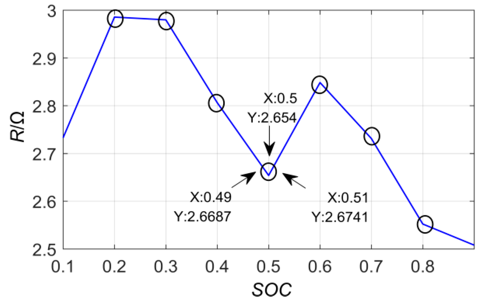
This paper reasonably optimizes the model parameters when the SOC is 0.1 X (where X is an integer from 1 to 9). In Figure 9, the ohmic resistance R₀ at the time when the experimentally measured SOC is equal to an integer multiple of 0.1 is shown.

When these raw data are substituted into the model for SOC estimation, there will be more abrupt changes or "spikes" in the variation curve of the parameters when the SOC is equal to an integer multiple of 0.1, as shown by the black circle in Figure 9. However, in actual continuous operation conditions, the change trend of each parameter of the battery is continuous and relatively flat, without an obvious inflection point. To make the data curve as flat as possible on the premise of approaching the real value, reasonable methods are considered to optimize the data measured in the test to eliminate the spike. Conventional polynomial fitting results in a very smooth fitting curve, but often has a large deviation from the true value, and the error trend at both ends of the curve is the most serious.

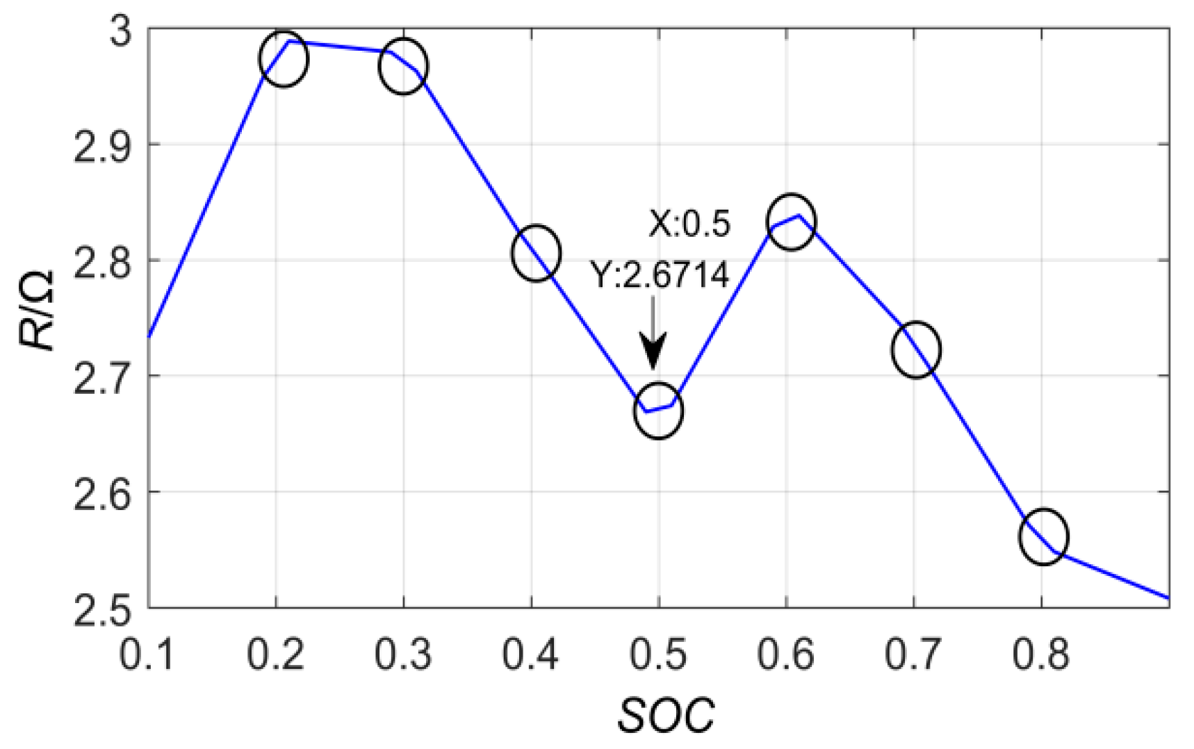
Given the data accuracy and the slowly changing curve characteristics, this paper adopts a reasonable optimization method to weaken data mutation. In time, $SOC=0.1X$($X=1,2\dots \dots 9$), the model parameters are the identified real values, and the model parameters are optimized before and after 0.1 X. That is, point $(0.1X-0.01)$ and point $(0.1X+0.01)$ are selected around point $SOC=0.1X$ to optimize the model parameters of the point $SOC=0.1X$. When $SOC=(0.1X-0.01)$, the model parameter values at times $SOC=0.1X$ and $SOC=(0.1X-0.1)$ are connected by a straight line, and the model parameter value at time $SOC=(0.1X-0.01)$ is obtained by the functional relationship of the straight line and set as $m$. When $SOC=(0.1X+0.01)$, the model parameter values when $SOC=0.1X$ and $SOC=(0.1X+0.1)$ are connected by a straight line, and the model parameter value at time $SOC=(0.1X+0.01)$ is obtained as $n$ according to the functional relationship of the straight line. $(m+n)/2$ is taken as the optimal value of the model parameter at time $SOC=0.1X$. After optimization, there is a small error in the model parameters at $SOC=0.1X$, but, in return, the model parameters are closer to the curve of continuous changes in the actual working conditions.

The data curve of the battery internal resistance $R0$ measured at 25 °C and $SOC=0.5$ is taken as an example. The $R0$ values of group $SOC=0.49$ and group $SOC=0.51$ are selected as model reference data before and after the mutation point, and the average value of the times $SOC=0.49$ and $SOC=0.51$ are calculated as the analysis values of the original "peak" point. The obtained optimized data curve is shown in Figure 10.

From the optimized data curve, it can be seen that each data mutation and spike is weakened or smoothed, making the change trend of each parameter of the model closer to the actual operating conditions of the EVs. Similarly, the rest of the model parameter data are reasonably optimized (where the $V_{oc}$ original data curve is relatively smooth and will not be optimized).

5. Comparison of Online SOC Estimation before and after Model Parameter Optimization

The verification of the AUKF based on the optimization of the model parameters is divided into three aspects. First, the estimation accuracy of the AUKF is compared to that of the normal UKF. Second, the superiority of the AUKF estimation accuracy before and after the optimization of the model parameters is verified. Finally, the convergence of the AUKF to the initial value error of the SOC before and after the optimization of the model parameters is verified.

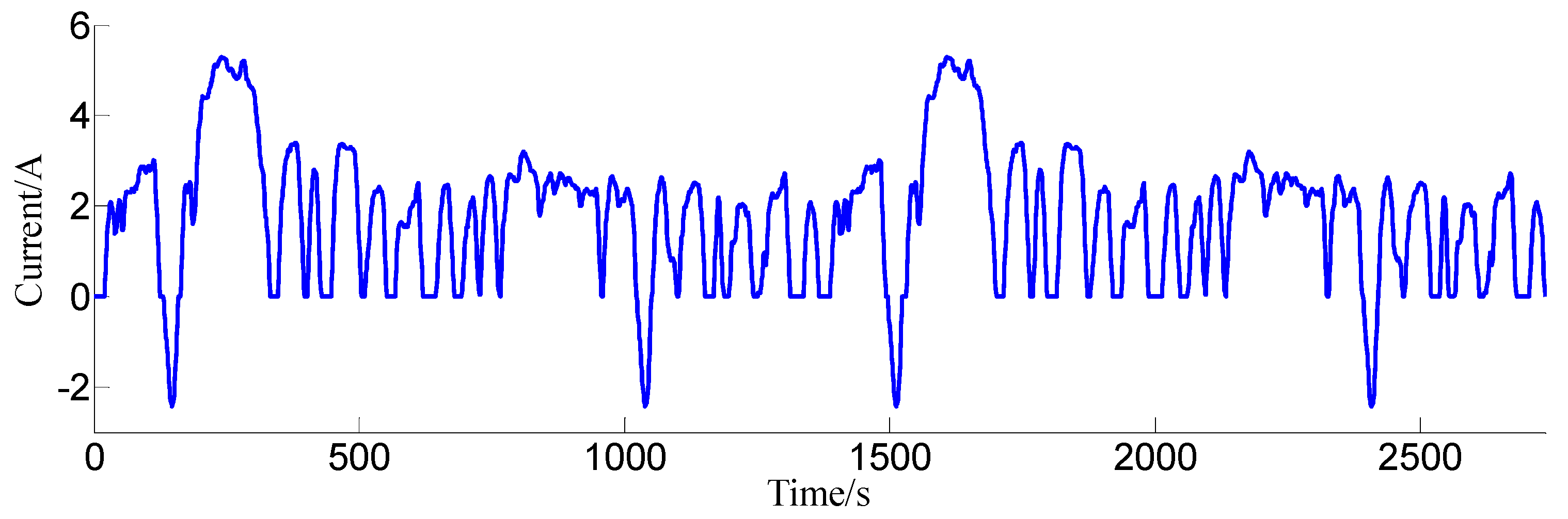
In the process of setting the battery charge and discharge state, the UDDS (Urban Dynamometer Driving Schedule) waveform [27] is used as a reference. To ensure correspondence with the experimental object (SANYO 18650 Li-ion battery) in the process of OCV–SOC calibration, the current signal in Figure 11 is adopted to describe the increase or decrease of the current in the discharging or charging process of the power battery. In one period, the average output current is 1.77 A, the maximum discharging current is 5.28 A, and the maximum charging current is 2.42 A. Each period is 1367 s, and the condition lasts for two periods.

5.1. Comparison of the Estimation Accuracy between the AUKF and the UKF

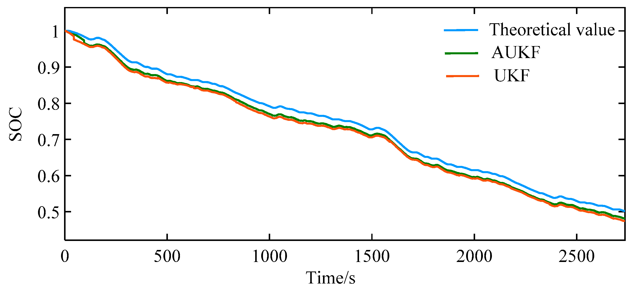
The third section explains in detail the process of establishing the AUKF. This section verifies the superiority of the AUKF and the UKF in terms of estimation accuracy in MATLAB/Simulink. The verification process is based on the model parameters before optimization. In this simulation model, the input current I(k) is integrated using the ampere-hour integral method. As there is no error in the current measurement due to outside disturbances, no accumulative error exists. Thus, the integration of the current in the simulation model can be regarded as the theoretical value of the SOC. 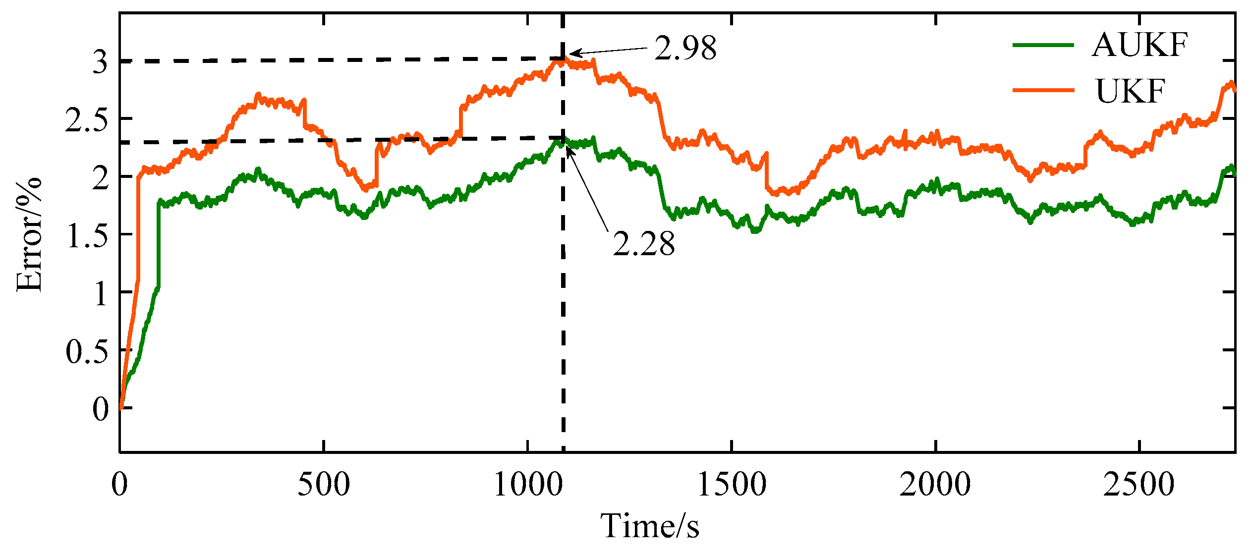The model simulation results and errors are shown in Figure 12 and Figure 13, respectively.

From the simulation results, the AUKF and the UKF can estimate the SOC online well under different charge and discharge rates. The UKF maximum estimation error is 2.98%, and the maximum estimated error of the AUKF is 2.28%; compared with the UKF, its estimation accuracy is significantly improved.

5.2. Comparison of the AUKF Estimation Accuracy before and after Optimization of the Model Parameters

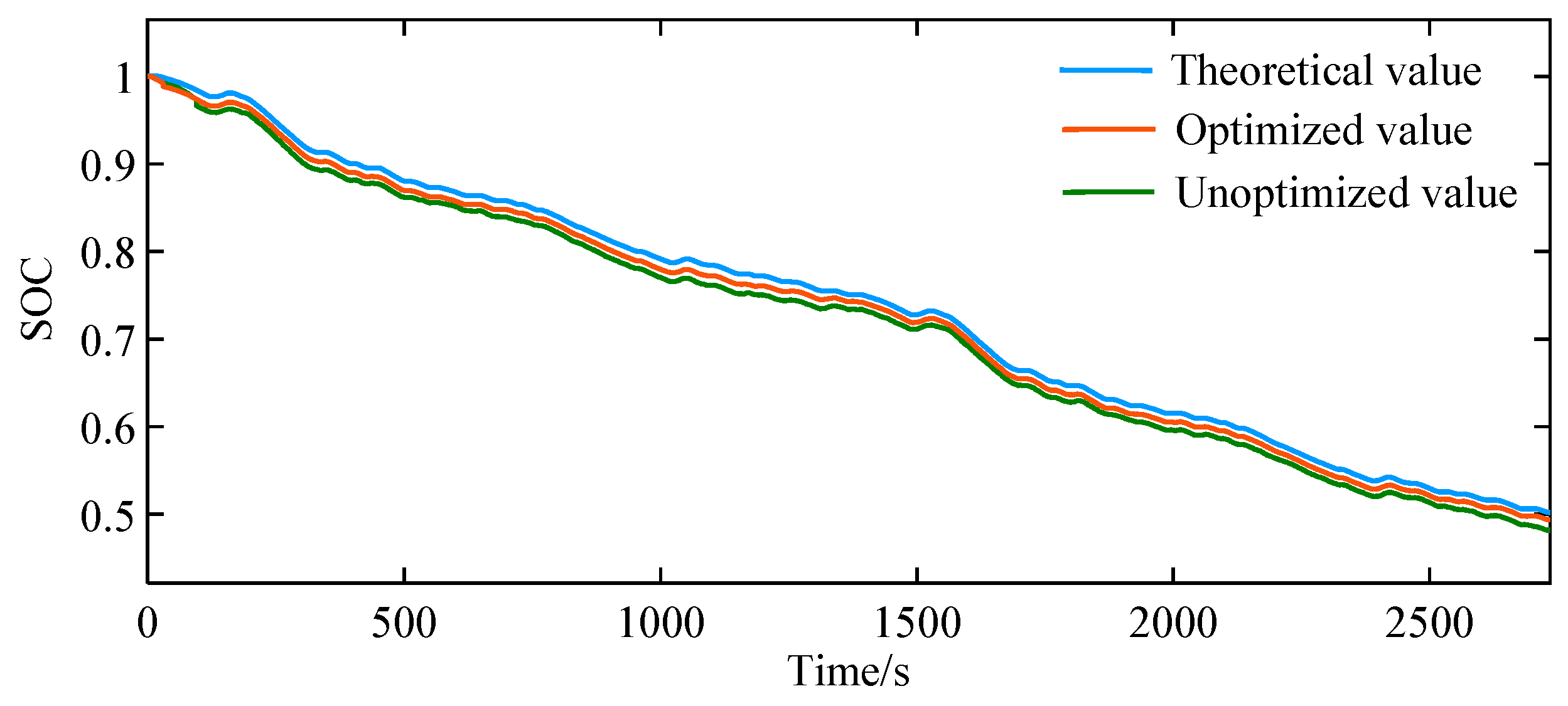
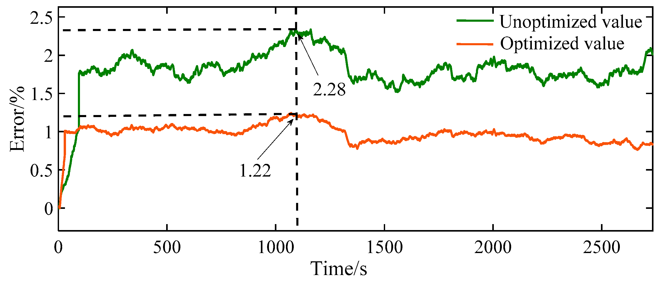
Substituting the optimized model parameters into the AUKF simulation model, the results are compared with the estimated values before the optimization of the model parameters. The simulation output is shown in Figure 14, and the error is shown in Figure 15.

From the simulation results shown in Figure 14 and Figure 15, the online estimation of the SOC is closer to the theoretical value after the reasonable optimization of the model parameters. The maximum SOC estimation error obtained after optimization of the model parameters is 1.22% and compared to the maximum error of 2.28% before parameter optimization, the error decreases significantly. It is verified that the optimization process can significantly improve the online estimation accuracy of the AUKF based on the original data.

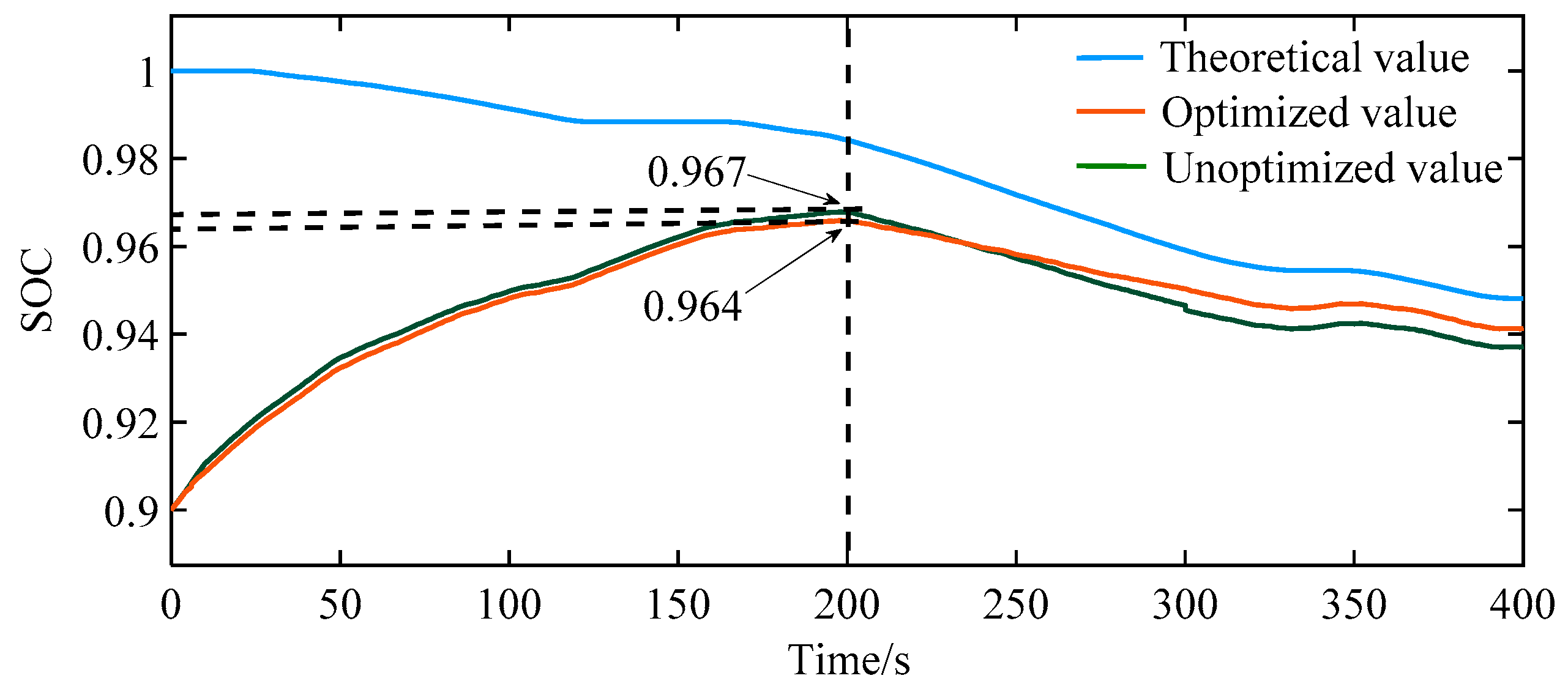
5.3. Convergence Comparison of the Initial Error of the AUKF before and after Parameter Optimization

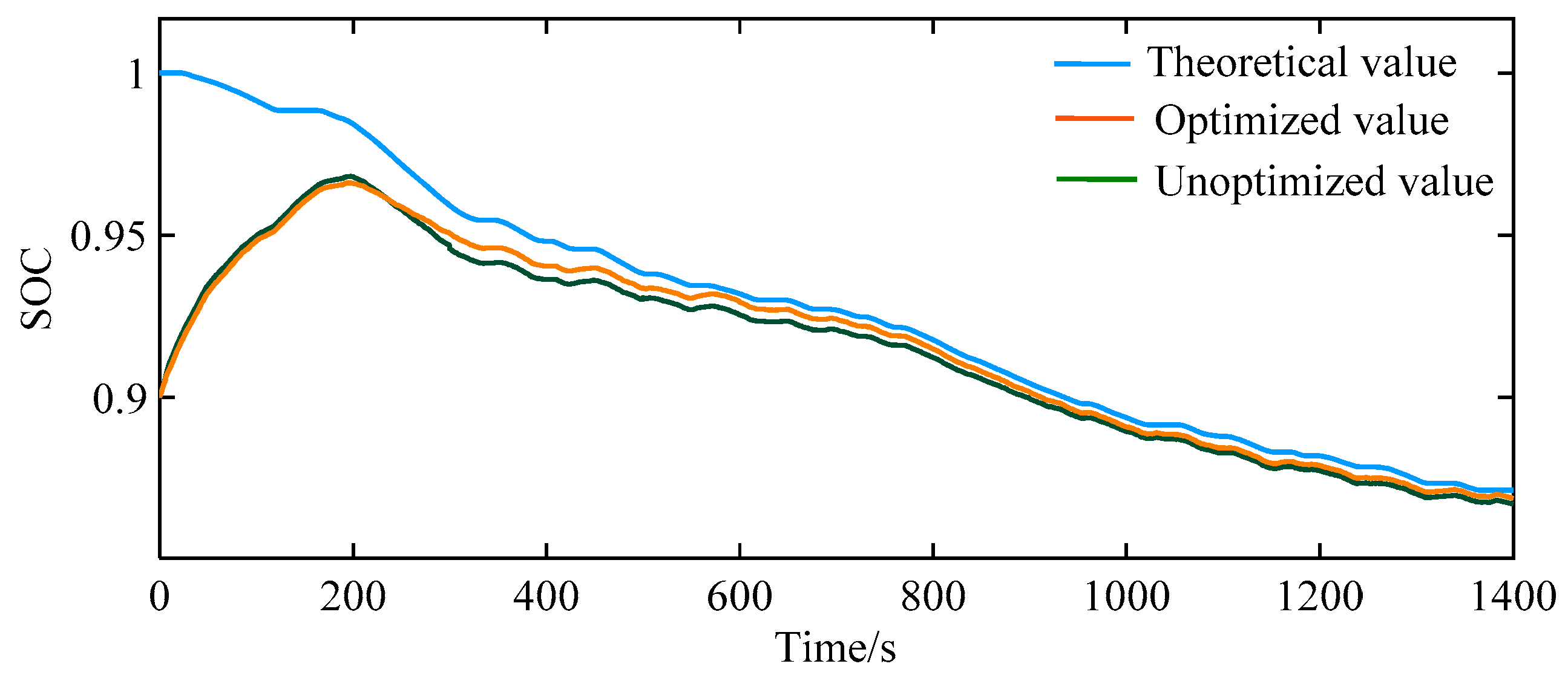
The Kalman filter has a strong convergence effect on the initial error of the SOC. This section verifies the effect of the reasonable optimization of the model parameters on the initial error convergence ability of the AUKF. The initial value of the system state SOC in the AUKF is set to the same value, and the output of the AUKF estimation before and after model parameter optimization is compared. The initial SOC value is 0.9, and the simulation lasts for one cycle. A waveform comparison between the SOC value of the simulation model and the theoretical value is shown in Figure 16. Figure 17 shows the convergence of the initial error before and after the model parameter optimization of the first 400 s. The SOC estimation values before and after optimization at 200 s are given.

As seen from Figure 16, before and after model parameter optimization, the SOC values estimated by the AUKF converge to the theoretical value quickly. In Figure 17, at 200 s, the estimated value before optimization is 0.967, which is closer to the theoretical value than the optimized estimated value of 0.964, but the difference is only 0.003; that is, the difference is only 0.3%, which can be ignored. This shows that the convergence ability of the AUKF algorithm to the initial error before and after optimization of the model parameters is approximately the same, and optimization of the model parameters has no effect on the convergence of the algorithm.

6. Conclusions

The SOC provides vital state information for EVs and is strongly nonlinear and time-varying. For the purpose of the accurate online estimation of the SOC, the parameters of a second-order RC equivalent circuit model are identified by combining circuit principles and optimized rationally. The AUKF with optimized model parameters is used to estimate the SOC. The conclusions of this work can be summarized as follows:

• The second-order RC model is proven to be the most suitable equivalent circuit model compared with the Thevenin and multi-order models.
• The covariances of the process noise and the measurement noise of the UKF are updated in real time to improve the accuracy of SOC estimation.
• A reasonable optimization method is adopted to weaken model parameter mutation. Optimized parameters can significantly improve the online estimation accuracy of the AUKF based on the original data and have little effect on the convergence of the algorithm.

In the future, to further improve the accuracy of SOC estimation, the influence of temperature and SOH on SOC estimation must be considered.