Article

An Initial Value Estimation Method for the Kalman and Extended Kalman Filters in Underground Metal Detection

1
School of Computer and Communication Engineering, University of Science and Technology Beijing, Beijing 100083, China
2
Sunkaisens(Beijing) Technology, Ltd. China, Hangfeng Road, Fengtai District, Beijing 100071, China
3
NetEase, 599 Shangshang Road, Binjiang District, Hangzhou 310052, Zhejiang, China
4
School of Mathematics and Physics, University of Science and Technology Beijing, Beijing 100083, China
5
School of Materials Science and Engineering, University of Science and Technology Beijing, Beijing 100083, China
*
Author to whom correspondence should be addressed.
Appl. Sci. 2019, 9(19), 4113; https://doi.org/10.3390/app9194113
Submission received: 21 August 2019 / Revised: 22 September 2019 / Accepted: 25 September 2019 / Published: 1 October 2019

Abstract

:
As an underground metal detection technology, the electromagnetic induction (EMI) method is widely used in many cases. Therefore, the EMI detection algorithms with excellent performance are worth studying. One of the EMI detection methods in the underground metal detection is the filter method, which first obtains the secondary magnetic field data and then uses the Kalman filter (KF) and the extended Kalman filter (EKF) to estimate the parameters of metal targets. However, the traditional KF methods used in the underground metal detection have an unsatisfactory performance of the convergence as the algorithms are given a random or a fixed initial value. Here, an initial state estimation algorithm for the underground metal detection is proposed. The initial state of the target’s horizontal position is estimated by the first order central moments of the secondary field strength map. In addition, the initial state of the target’s depth is estimated by the full width at half maximum (FWHM) method. In addition, the initial state of the magnetic polarizability tensor is estimated by the least squares method. Then, these initial states are used as the initial values for KF and EKF. Finally, the position, posture and polarizability of the target are recursively calculated. A simulation platform for the underground metal detection is built in this paper. The simulation results show that the initial value estimation method proposed for the filtering algorithm has an excellent performance in the underground metal detection.

1. Introduction

Underground metal detection technology has been widely used in military fields [1] and also plays an important role in archeology [2], prospecting [3], medical positioning [4], underground metal pipeline modeling [5] and other fields. Electromagnetic induction (EMI) detection technology is an underground metal detection method that uses secondary field information generated by a changing magnetic field acting on the metal target to detect the state of a target [6]. In the EMI model, the secondary field is related to nine parameters of a target, which are grouped into the target’s position r = r x r y r z T , polarizability β = β x β y β z T , and posture ψ θ ϕ T [7]. ψ , θ , ϕ are the yaw angle, pitch angle and roll angle of the target, respectively. Compared with other underground metal detection technologies, such as infrared imaging and seismic wave technology, EMI detection technology has the advantages of having a strong penetration capability and being nondestructive [8], so it is widely used in the underground metal detection field. EMI technology includes time domain electromagnetic (TDEM) induction [9,10] and frequency domain electromagnetic (FDEM) induction [11]. In the TDEM method, a pulse signal is transmitted. Then, the position and polarizability of the target are obtained by analyzing the attenuation characteristics of the secondary field signal. Unlike the TDEM method, the FDEM method transmits harmonic signals with multiple frequencies. Through analyzing the amplitude and phase information of the secondary field signal, the position, polarizability and posture of the target can be obtained. Both TDEM induction and FDEM induction are based on the same fundamental physical principles, but the types of information obtained from secondary fields are different. The FDEM method measures the phase and amplitude of the secondary fields, which is different from the primary fields, mainly due to the subsurface properties [12]. We focus on the FDEM method in this paper.
Inversion algorithms are used to calculate the target’s physical parameters from the observed data. It includes recursive inversion algorithms [8,13] and nonrecursive inversion algorithms [1,14]. For example, filter methods are classified as recursive inversion algorithms, and gradient methods are classified as nonrecursive inversion algorithms. The filter method uses the system’s dynamic state space model (DSSM) to solve the target detection problems and offers good real-time performance. Filter algorithms mainly include particle filters (PFs) and Kalman filters (KFs). When PFs are in the face of high-dimensional problems such as dipole tracking, the number of required particles increases exponentially, which results in the “curse of dimensionality”. When the noise satisfies the Gaussian distribution, the KFs have the best performance, and this assumption is also reasonable in practical applications. Consequently, we focus on KFs in this paper. Although nonrecursive inversion algorithms have higher accuracy than recursive algorithms, their computational efficiency is lower than that of filter algorithms. We focus on improving the accuracy of KF algorithm in underground target detection.
Filter methods have long been used to solve underground metal detection problems. For example, Grzegorczyk et al. used a KF and an extended Kalman filter (EKF) to solve the problem of underground unexploded ordnance detection [8]. However, in the traditional EMI model, the secondary field of the target has a nonlinear relationship with six parameters that relate to the position and posture and has a linear relationship with the three parameters of polarizability. The high nonlinearity of the model results in poor performance of the filter algorithm. Dekdouk et al. used the concept of the magnetic polarizability tensor to reduce the number of nonlinear parameters from six to three in the traditional model [15]. Ambruš et al. used a linearized model to solve the problem of underground metal detection [16]. However, one problem that cannot be avoided in the current research is that the performance of filter algorithms is extremely sensitive to the initial value of the filter. In the case of a large initial value error, the precision is low, and the results sometimes are divergent. In [17], Chan et al. used a least squares estimator to yield an estimation of the acceleration input vector for maneuvering targets. In [18], Koopman used maximum likelihood estimation to solve the initialization problem of the KF. Based on their research, the least squares method and two image processing algorithms are combined to obtain initial values for the filter algorithm in underground metal detection. Early research in the underground metal detection is mostly based on the assumption of Gaussian noise distribution. Tomasz et al. investigate KF and EKF for the inversion of unexploded ordnance (UXO) polarizabilities and positions under the dipole model approximation and the assumption of Gaussian noise distribution, respectively [19]. There are also some researchers studied the application of detection algorithm in non-Gaussian noise. Tantum et al. studied the effects of assuming i.i.d. white Gaussian noise on the performance of likelihood ratio detectors and maximum likelihood classifiers implemented in a non-Gaussian noise environment. In addition, they had illustrated the effects of mismatch between the assumed and actual noise distributions on detection and classification performance for likelihood ratio processors derived under several assumptions regarding the noise distribution [20]. Gordon et al. had proposed the bootstrap filter for implementing recursive Bayesian filters [21]. In addition, the method is not restricted by assumptions of linearity or Gaussian noise. In [22], Jay et al. derived a theoretical expression of the optimum non-Gaussian radar detector. The researchers above had made certain research about non-Gaussian noise. In this paper, we focus on the improvement of the filter algorithm’s performance in the environment of non-Gaussian noise.
In this paper, we propose an initial value estimation method for the KF and the EKF (IVE-KF) for underground metal detection. In IVE-KF, the horizontal position of the target is estimated by the first-order central moments of the map that are composed of secondary field data, the depth of the target is estimated by the full width at half maximum (FWHM), and the initial states of the other six linear parameters are estimated by the least square method combined with Tikhonov regularization. Finally, these initial states are used as the initial values of the filter algorithm, and the parameters of the metal target are solved simultaneously by combining the KF and the EKF algorithms. To evaluate the performance of IVE-KF, a simulation platform for EMI detection is built in this paper. The simulation results show that the convergence of IVE-KF is better than that of the filter algorithm with random initial values in the application of underground metal detection, and the detection accuracy is close to that of the Levenberg–Marquardt (LM) algorithm of inversion when the signal-to-noise ratio (SNR) is greater than 30 dB; in addition, the computational complexity of IVE-KF is lower than that of the LM algorithm.
The detailed content of this paper is arranged as follows: Section 2 introduces the system model. Section 3 introduces the IVE-KF algorithm, which includes the initial value estimation algorithm and the filter algorithm. Section 4 introduces the simulation system and evaluates the performance of the IVE-KF algorithm. Section 5 concludes the paper.

2. System Model

Notation: In this paper, bold letters denote vectors and matrices; ω omega denotes the angular frequency of electric current in the transmitter; w denotes the number of sets of secondary field data we collected in the process of detection; H P , B P and B s respectively denote the values of the primary field magnetic field intensity, primary field magnetic induction and secondary field magnetic induction, which contain x, y, and z components; C denotes the collected secondary field data generated by the simulation system; θ , ϕ , and ψ denote the pitch angle, roll angle and yaw angle for a vertically placed cylinder target, respectively; and j denotes the imaginary unit.
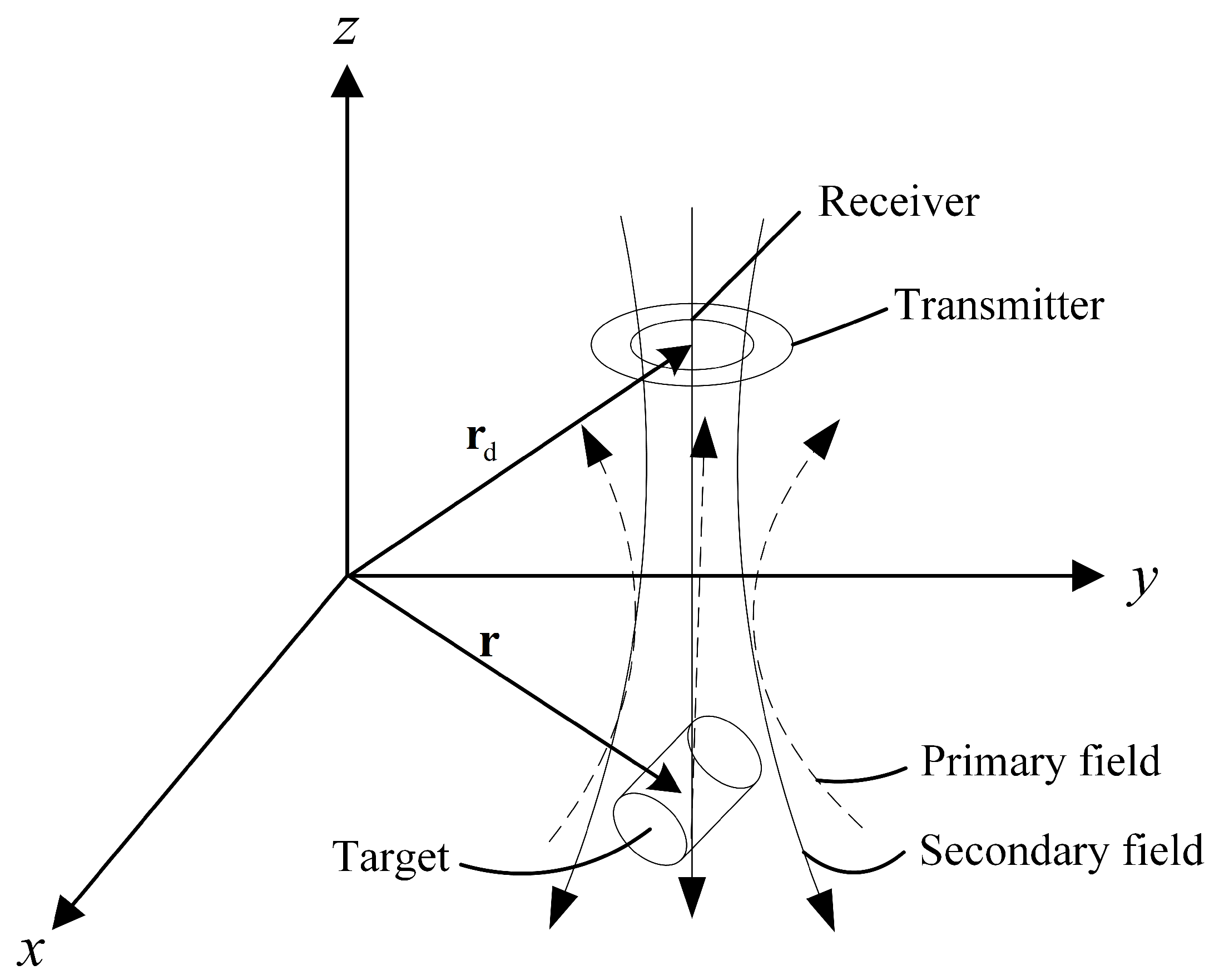
In the detection system, the metal target is located at a certain position in the underground space. When the primary field (generated by the transmitter) acts on the metal target, a secondary field is generated by the eddy current of the metal target. The secondary field data are collected by a detector sequentially placed in different positions on the detection plane (the detector includes a transmitter and a receiver; in this paper, we assume that these two components are coincident). Estimation of the target’s parameters can be obtained from these secondary field data. As shown in Figure 1, in EMI detection, the commonly used data collection scheme is 2D scanning [14,23,24]. The detector is placed on the scanning line to collect data successively. On each scanning line, the distance between two adjacent sampling points is called the point interval p s , and the distance between the scanning lines is called the line interval l s . The plane where the scanning line is located is called the detection plane. Assuming that there are 2 M + 1 scanning lines, 2 N + 1 sets of data are collected on each scanning line, ultimately producing w = ( 2 M + 1 ) ( 2 N + 1 ) sets of data collected on the detection plane. Each set of data are represented by C k ( k = 1 w ) . Based on these collected data, the initial value estimation algorithm can be used to obtain the approximate estimation of the target state, and, by using these initial values, an accurate estimation of the metal target’s parameters can be obtained quickly by the KF and EKF algorithms. In Figure 1, the target position vector is r , the posture is ψ , θ , ϕ , and the polarizability is β = β x β y β z T . To obtain an estimation of the target’s parameters from secondary field data, it is necessary to characterize the EMI response with a suitable forward model.
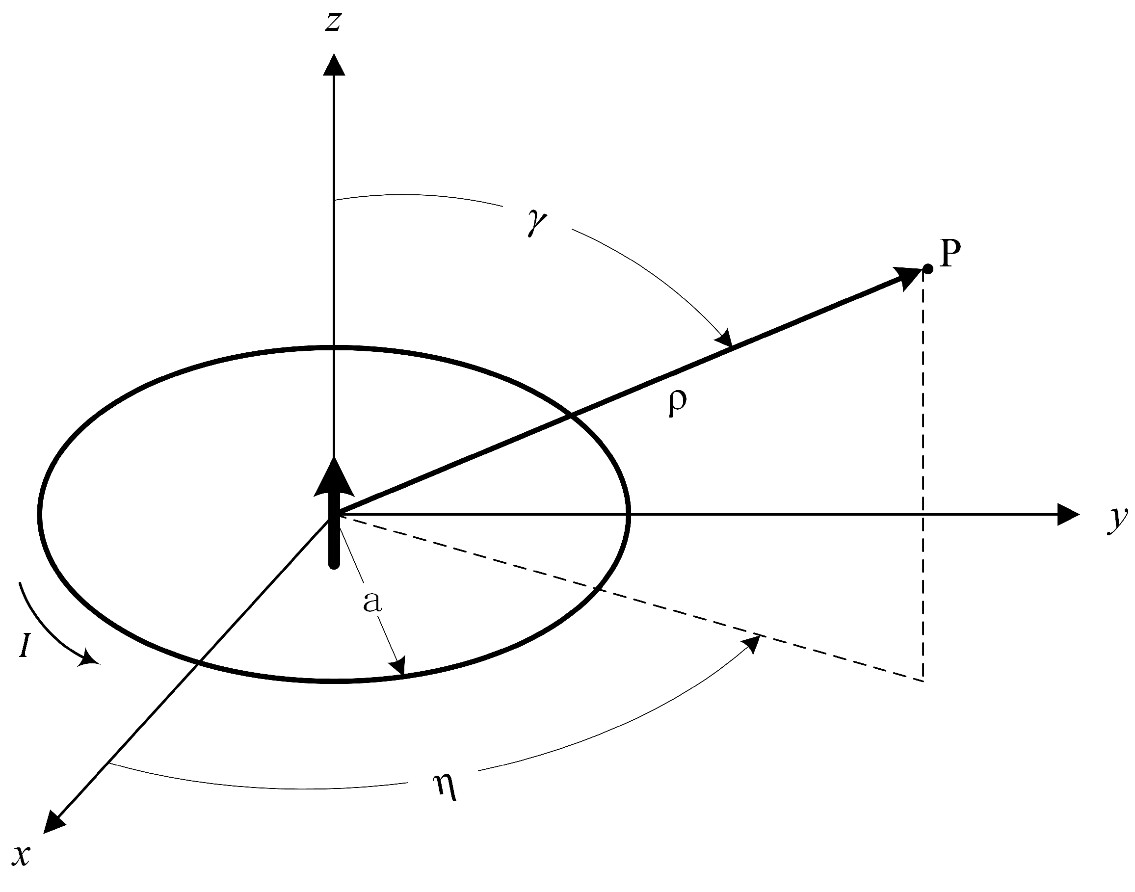
A spherical coordinate system is used in the primary field calculation because calculating the primary field in this coordinate system is simpler than that in a Cartesian coordinate system. As shown in Figure 2, there is a circular coil with a radius of a in the space, and a harmonic current I = I 0 e j ω t with an angular frequency of ω is applied to the coil. In the spherical coordinate system, the center of the toroidal coil lies at the origin. ρ , γ , η are the radial distance, polar angle and azimuthal angle, respectively. The inducted field strength at any position P ( ρ , γ , η ) in space is [25]:
H ρ = j μ 0 k r a 2 I 0 cos γ 2 ρ 2 1 + 1 j k r ρ exp j k r ρ ,
H γ = μ 0 k r a 2 I 0 sin γ 4 ρ 1 + 1 j k r ρ 1 k r ρ 2 exp j k r ρ ,
H η = 0
where μ 0 is the vacuum permeability, k r = 2 π λ is the wave number of electromagnetic waves in the propagation medium, λ = 2 π v ω is the wavelength of the electromagnetic waves, and v is the wave velocity in the medium. Then, the spherical coordinates can be converted to rectangular coordinates according to Formula (4):
H x = H ρ sin γ cos η + H γ cos γ cos η H η sin η , H y = H ρ sin γ sin η + H γ cos γ sin η + H η cos η , H z = H ρ cos γ H γ sin γ .
The principle of electromagnetic induction in underground metal detection is illustrated by Figure 3, the detector position is r d , and the target position is r . When the length of the detected target is much shorter than the distance between the detector and the detected target, the detected target can be idealized as a magnetic dipole, which satisfies the requirements of engineering applications. When the primary field acts on the metal target, an eddy current is generated inside the metal. The magnetic field sensor can be used to obtain the secondary field B s generated by the eddy current [26]:
B s = μ 0 4 π 3 m · r r r 5 m r 3 ,
where m is the induced dipole moment at the metal target position, μ 0 is the permeability of vacuum, r is the distance from the detector center to the metal target center, and r is the vector of the metal target center pointing to the detector center. The value of the induced dipole moment is related to the detected target’s posture and polarizability and the primary field strength [26]:
m = U β U T H P ,
where U T represents the transpose of the matrix U and U is the transformation matrix between the observation coordinate system and the metal target coordinate system, also known as the Euler rotation matrix [27]. H P = H x H y H z T is the primary field strength calculated according to Formulas (1)–(3) at the detected target position. β , the polarizability of the metal target, is an intrinsic feature of the target and is independent of the position and posture:
β = β x 0 0 0 β y 0 0 0 β z .
Formulas (5) and (6) imply that the secondary field has a nonlinear relationship with the position and posture angle of the detected target and scales linearly with the polarizability. Therefore, a nonlinear equation needs to be solved to obtain the position and posture angle, which is a relatively complicated undertaking. In [15], Formula (6) is written as follows:
m = M H P ,
where M is a 3 × 3 magnetic polarizability tensor, which is related to the polarizability and posture of the metal target. M fully reflects the dipole response of the metal target and it can be proven that M is a 3 × 3 symmetric matrix [28]; thus, there are only six different elements in M . M can be expressed as follows:
M = M 11 M 12 M 13 M 12 M 22 M 23 M 13 M 23 M 33 .
Magnetic polarizability tensor M is related only to the posture and the polarizability of the target; therefore, it is constant during the detection process. M can be directly obtained from the secondary field data without obtaining the target’s polarizability and three posture angles. Because the secondary field strength and M are linearly related, the use of M reduces the number of nonlinear parameters in the EMI model and greatly improves the computational efficiency in the calculation process. Once the six parameters in M are obtained, the polarizability β and the three posture angles can be obtained directly. Eigendecomposition is performed on M to obtain:
M = U U 1 ,
where ∑ is a diagonal matrix, each element on the diagonal line is the eigenvalue of M , and β are the elements on the diagonal line of ∑. Since M is a symmetric matrix, U T = U 1 , and the corresponding posture angles can be obtained:
θ = si n 1 U 13 ,
ϕ = si n 1 U 23 cos θ ,
ψ = co s 1 U 11 sin θ .
Finally, the secondary field is represented as (with the constant being omitted for conciseness):
B s r , r d , ψ , θ , ϕ , β = Gm = G M B P ,
where r and r d are the position vectors of the detected target and detector, respectively. ψ , θ , and ϕ are the posture angles of the target, β = β x , β y , β z T is the target’s polarizability, μ 0 is the permeability of vacuum, G is Green function, which is related only to the position vector r d r , M is the magnetic polarization tensor, B P is the primary field magnetic induction at the detected target and B P = μ 0 H P , and μ 0 is the permeability of vacuum.
The Formula (14) can be further abstracted as:
B s = F α ,
where α = [ x , y , z , M 11 , M 22 , M 33 , M 12 , M 13 , M 23 ] is a nine-dimensional vector and x, y and z are the positions of the target object in the coordinate system.

3. IVE-KF Algorithm

The metal target parameters in the process of detection can be considered equivalent to a state vector in a dynamic system. Since the noise can be approximated by a Gaussian distribution during the detection process [8], the KF method can be used to predict the state information of the metal target. However, since the optimized model still has three nonlinear parameters related to the position, the EKF must be used to solve the nonlinear parameters in the model. The EKF uses the first derivative in the Taylor series to approximate the nonlinear function of the model. Therefore, in the detection process, the linear and nonlinear parameters in the target state vector are estimated by KF and EKF, respectively. However, the performance of the KF algorithm is sensitive to its initial value. In the case of a large initial value error, the filtering accuracy is low, and the results are sometimes divergent. In order to overcome this problem, it is necessary to provide an initial value α ^ 0 that is relatively accurate for the filter algorithm. α ^ 0 contains the position estimation and magnetic polarizability tensor estimation of the metal target.

3.1. Initial Value Estimation

In the data collection process, the detector is evenly distributed on the detection plane. The detector position is denoted by r d , and the area of the detection plane is 2 N + 1 p s × 2 M + 1 l s . After all data are collected on the detection plane, the secondary field strength at each r d k ( k = 1 w ) is calculated. The secondary field strength map is composed of these data. According to the secondary field strength map, a relatively accurate estimation of the metal target’s parameters is obtained. The horizontal position estimation is [29]:
X ^ 0 , Y ^ 0 T = Hor r a r g m a x C k ,
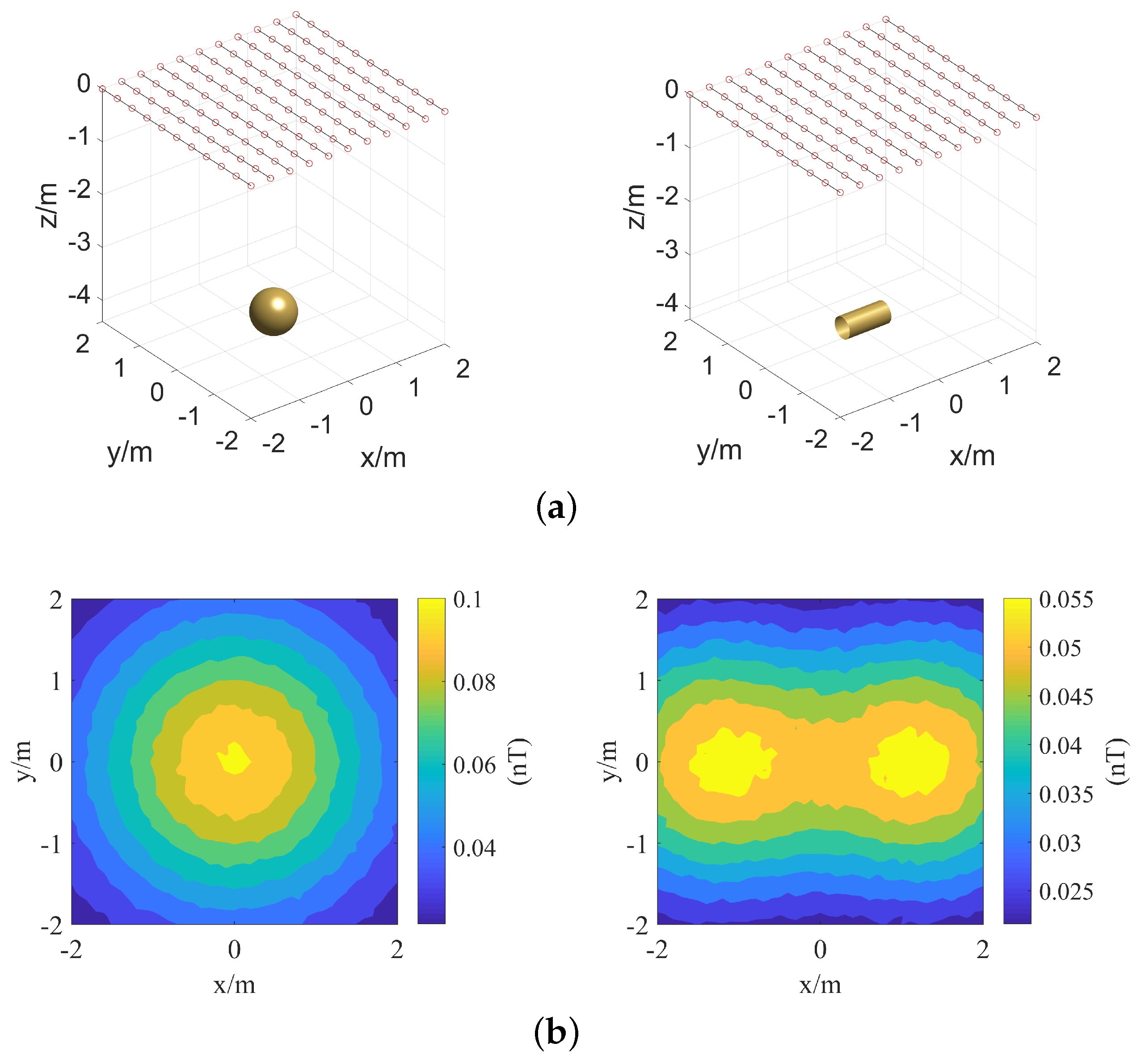
where X ^ 0 , Y ^ 0 is the estimation of the target’s x-coordinate and y-coordinate, a r g m a x · is used to obtain the variable value when the function reaches its maximum value, C k is the collected data, and Hor r represents the horizontal component of the position vector r . The secondary field strength maps of the sphere and the cylinder objects are shown in Figure 4.
When the detected target is a sphere of uniform material, a circular bullseye shape occurs in the secondary field strength map, and the position of maximum strength is exactly the horizontal position of the spherical target, as shown on the left side of Figure 4. However, for cylindrical targets in different postures, the secondary field strength map is asymmetrical and may have multiple local maxima, as shown on the right side of Figure 4. In such a case, an inaccurate estimation of the target’s horizontal position is obtained according to Formula (16). To make the algorithm more universal, the first-order central moment of the secondary field strength map is used to estimate the initial state of the target’s horizontal position in this paper [30]:
X ^ 0 = i = 1 w C k X k i = 1 w C k , Y ^ 0 = i = 1 w C k Y k i = 1 w C k ,
where X k and Y k are the x-axis component and the y-axis component of the detector position r d k , respectively.
The FWHM method is used to estimate the depth of the target [31]:
Z ^ 0 = 2 S π ,
where S is the area in which the value is greater than half of the maximum value on the secondary field strength map. After depth estimation, the target’s initial position vector r ^ 0 = X ^ 0 Y ^ 0 Z ^ 0 T is obtained. According to Formula (14), the secondary field strength B s , Green function G , magnetic polarizability tensor M and primary field strength B P are all linearly related. G can be calculated according to the detector’s and target’s positions, and B P can be calculated according to Formulas (1)–(3); thus, M can be directly calculated by the linear equation:
M B P = G 1 B s .
The magnetic polarizability tensor M is a symmetric matrix with six different parameters. In practice, only three sets of equations can be obtained from a set of collected data, so at least two sets of collected data are needed to calculate the six parameters M 11 , M 22 , M 33 , M 12 , M 13 , M 23 and the sets of data we collected are much more than two sets. Therefore, as long as the position estimation of the detected target is obtained, the other six parameters can be obtained.
Assuming that the kth set of data C k is collected, let T k = G 1 C k = T x k , T y k , T z k T , with primary field strength B p k = B x k , B y k , B z k T , and then combine the Formulas (9) and (19):
M 11 B x k + M 12 B y k + M 13 B z k = T x k , M 12 B x k + M 22 B y k + M 23 B z k = T y k , M 13 B x k + M 23 B y k + M 33 B z k = T z k .
Formula (20) can be written in matrix form [9]:
B x k 0 0 B y k B z k 0 0 B y k 0 B x k 0 B z k 0 0 B z k 0 B x k B y k M 11 M 22 M 33 M 12 M 13 M 23 = T x k T y k T z k .
For simplicity, Formula (21) is written as:
W k M 0 = T k ,
where M 0 = M 11 , M 22 , M 33 , M 12 , M 13 , M 23 T . When there are multiple sets of collected data C k 1 , C k 2 , . . . , C k L , let W = W k 1 T W k 2 T W k L T T , T = T k 1 T T k 2 T T k L T T . Formula (22) can be written as:
W M 0 = T .
When L = 2 , W is a square matrix and reversible, Formula (23) has a unique solution:
M ^ 0 = W 1 T .
When L > 2 , Formula (23) becomes an overdetermined system. Due to the noise in the collected data, it is usually impossible to find a set of solutions M ^ 0 that strictly satisfy all the equations in Formula (23), that is, the equations have no solution. However, we can find a set of solutions M ^ 0 that satisfy all the equations in Formula (23) as much as possible:
M ^ 0 = arg min M 0 T W M 0 2 ,
where 2 is the Euclidean norm. Solving the above Formula, we can obtain:
M ^ 0 = W T W 1 W T T .
In the process of solving Formula (26), an ill-posed problem may occur, which leads to an obtained solution that has no practical significance. The reason for this problem is that W T W may be an ill-conditioned matrix [32]. A small error in the measured value is amplified by the ill-conditioned system, causing the solution to change drastically. Specifically, a small error in T causes the result M ^ 0 to be abnormal and to lose its practical significance. In this paper, the Tikhonov regularization method [33] is used to solve the ill-posed problem.

3.2. KF and EKF Algorithm

When the metal target’s initial state α ^ 0 has been estimated, the filter algorithm can be used to accurately estimate the metal target’s parameters.
Applying DSSM to the underground metal detection field produces unusual results because the state of the target (position, posture, and polarizability) is constant. Therefore, the changes in the state can be omitted:
α k = α k 1 + v k 1 ,
where α k is the state of the target so that when the kth set of data are collected, v k 1 consists of independent and identically distributed Gaussian noise. Formula (27) is called the state transition equation. The collected data at the kth sampling point are:
C k = F α k + n k ,
where F · is a nonlinear function for α . Formula (28) is called the observation equation.
In IVE-KF, the magnetic polarizability tensor M is estimated by the KF algorithm, and the target’s position r is estimated by the EKF algorithm. After the IVE-KF algorithm converges, the estimation of the target’s state α ^ k is obtained.
Assuming that the magnetic polarizability tensor of the target is M k when the kth set data are processed, according to (27) and (28), we can obtain:
M k = M k 1 + v k 1 ,
h k = F r , M k + n k = G k M k B P k + n k = G k W k M k + n k ,
where h k is the observed value, the target position r is considered as a known value, and G k is the Green function when the kth set of data are collected. W k is already defined in Formula (22). The KF algorithm for the magnetic polarizability tensor is [13]:
M k | k 1 = M k 1 | k 1 , P k | k 1 = Q k 1 + P k 1 | k 1 , M k | k = M k | k 1 + K k f , k C k G k W k M k | k 1 , P k | k = P k | k 1 K k f , k G k W k P k | k 1 ,
where the Kalman gain K k f , k is:
K k f , k = P k | k 1 G k W k G k W k P k | k 1 G k W k T + R k 1 .
Assuming that the position of the target is r k when processing the kth set of data, according to (27) and (28), we can obtain:
r k = r k 1 + v k 1 ,
h k = F r k , M + n k = G r d k r k M B P r k r d k + n k ,
where G · and B P · are both nonlinear functions for r , so r k needs to be calculated with the EKF algorithm [19]:
r k | k 1 = r k 1 | k 1 , P k | k 1 = Q k 1 + P k 1 | k 1 , r k | k = r k | k 1 + K e k f , k C k H k r k | k 1 , P k | k = P k | k 1 K e k f , k H k P k | k 1 ,
where the Kalman gain K e k f , k is:
K e k f , k = P k | k 1 H k H k P k | k 1 H k T + R k 1 .
H k is the Jacobian matrix of h k at r = r k | k 1 :
H k = h x k x h x k y h x k z h y k x h y k y h y k z h z k x h z k y h z k z ,
where h x , h y , and h z are the components of the secondary field on the x-, y-, and z-axes, respectively.
The process of the IVE-KF algorithm is shown in Table 1. After initial value estimation, the KF is used to predict and update the linear parameter M ^ with r ^ treated as a known value. Then, the EKF is used to predict and update the nonlinear parameter r ^ with M ^ being treated as a known value. After iteration, M ^ and r ^ ultimately converge. When the algorithm is completed, the estimation of the target parameters is obtained:
α ^ = r ^ T , M ^ T T .
α ^ contains the estimation information of the detected target’s position and the magnetic polarizability tensor. Formulas (9)–(13) imply that, once the M ^ is obtained, the polarizability β = β x , β y , β z T , and the posture angle ψ , θ , ϕ of the detected target can be easily obtained by eigendecomposition of the magnetic polarizability tensor M ^ .

4. Simulation Platform and Algorithm Performance

To verify the performance of the IVE-KF algorithm, an EMI detection simulation platform is built in this paper.
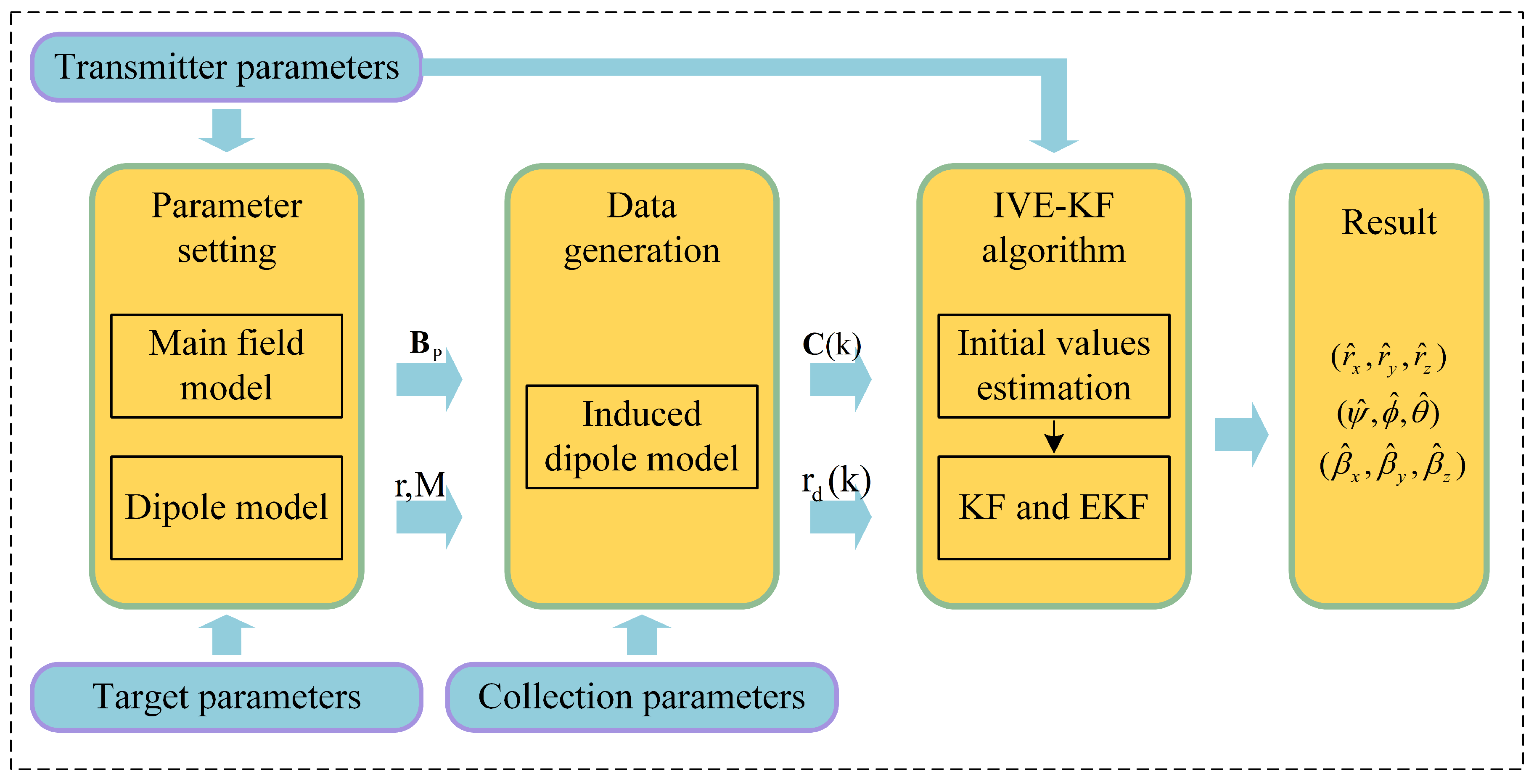
Figure 5 is the diagram of the simulation system. The transmitter parameters, target parameters and collection parameters can be set in the simulation system. According to the primary field model, the primary field B P at the detected target’s position can be obtained. Then, the target’s induced dipole moment and secondary field data C k at the detector position r d k can be obtained according to the induced dipole model. Finally, the generated data are processed by using the IVE-KF algorithm, and the parameters, including the position, posture and polarizability of the detected target are calculated. In Figure 5, the primary field model, the induced dipole model, and the IVE-KF algorithm are given as determined in Section 2 and Section 3. For irregular shaped targets, the calculation of the polarizability is very difficult, but, for spherical and cylindrical (axisymmetric) targets with uniform material, the process is relatively easy. The detected targets in the actual scene are mostly axisymmetric targets. Therefore, this paper selects a cylindrical object as the detected target to verify the feasibility and performance of the IVE-KF algorithm.
For a cylindrical target with radius a s and length L, let the length direction be the z-axis and radial direction be the x- and y-axis. The polarizability of the cylinder is [34]:
β x = β y = 1 2 V 0 . 35 + j ω τ 2 j ω τ + 1 ,
β z = LV 4 a j ω τ L 2 j ω τ L + 1 0 . 7 ,
where j is the imaginary unit 1 and σ is the conductivity of the target. μ and μ r are the magnetic permeability and relative permeability of the target, respectively. τ is the time constant, τ = a s 2 σ μ / μ r 2 , with τ L = 31 τ . The parameters to be set in the stimulation system are shown in Table 2, Table 3 and Table 4. In the subsequent simulation experiments, the simulation parameters are set as the values in these tables.
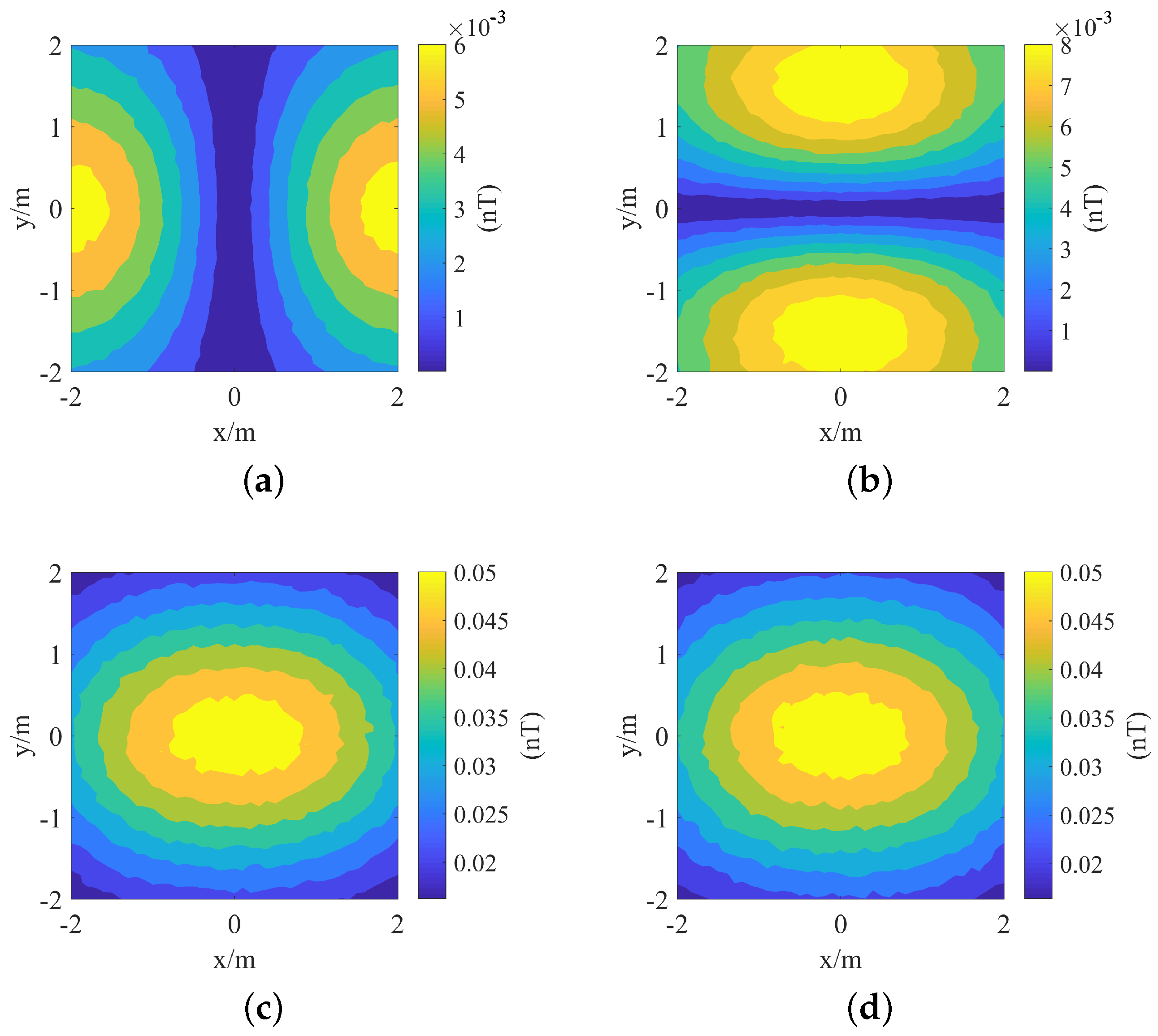
The secondary field strength map for the case in which a cylindrical target is parallel to the x-axis (that is, θ = 9 0 , as shown in Figure 6) is shown in Figure 7.
The maps of B x and B y are symmetric about the lines x = 0 and y = 0 , respectively. Considering that the B s response is consistent with the B z response but the amplitude of the B s is larger than the B z , B s is used in the following analysis.

4.1. Initial Value Estimation Performance

The performance of the initial value estimation algorithm is discussed from three aspects: horizontal position estimation performance, depth estimation performance, and magnetic polarizability tensor estimation performance. To objectively evaluate the horizontal position estimation performance, the horizontal position estimation errors at different simulation conditions are compared in this paper. The horizontal position estimation error u ¯ at each simulation condition is the average value obtained from 100 Monte Carlo experiments, which is:
u ¯ = i = 1 100 X ^ 0 i X 0 2 + Y ^ 0 i Y 0 2 100 ,
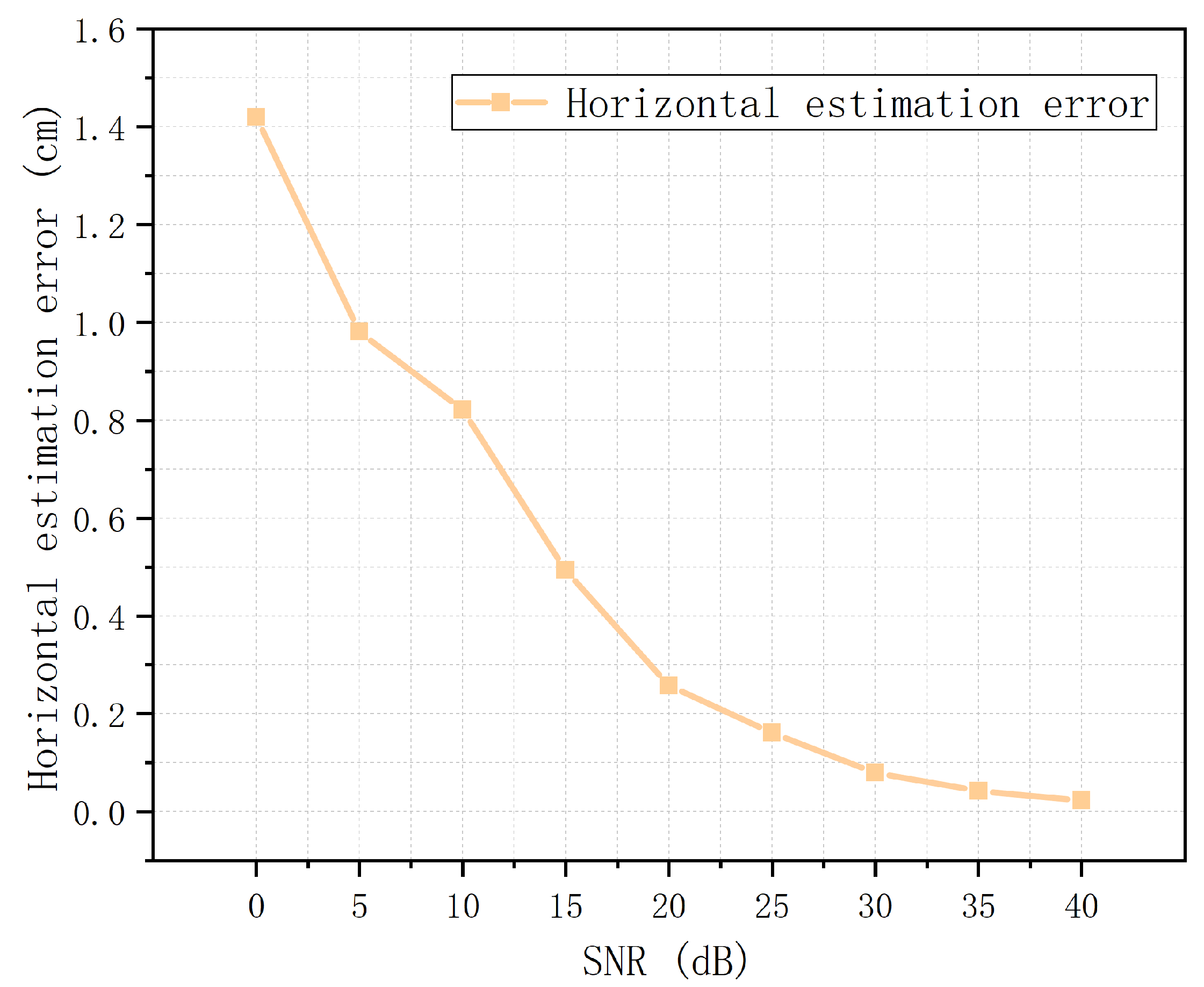
where X ^ 0 i , Y ^ 0 i is the horizontal position estimation obtained by the ith Monte Carlo experiment, and X 0 , Y 0 is the true position of the detected target. The results of the horizontal position estimation error for the cylindrical target at different S N R are shown in Figure 8. As S N R increases, the error gradually decreases. When S N R 10 dB, the error is less than 1 cm. The horizontal position estimation exhibits an excellent performance.
To evaluate the depth estimation performance, the depth estimation errors at different simulation conditions are compared in this paper. The depth estimation error d ¯ at each simulation condition is the average value obtained from 100 Monte Carlo experiments:
d ¯ = i = 1 100 Z ^ 0 i Z 0 100 ,
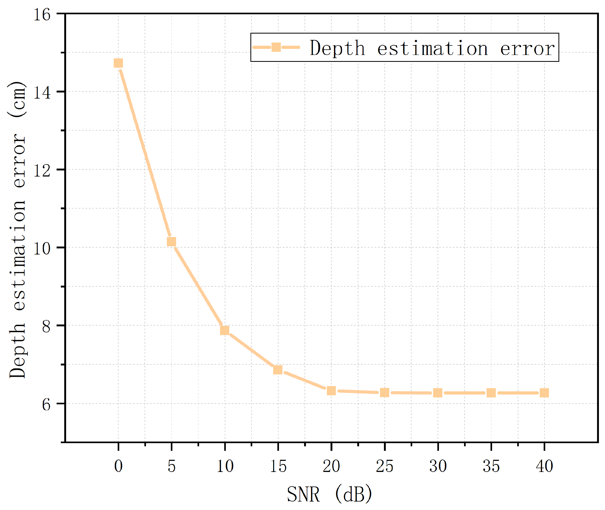
where Z ^ 0 i is the depth obtained by the ith Monte Carlo experiment and Z 0 is the true depth of the target. The depth estimation errors of cylindrical targets at different S N R are compared in Figure 9. It can be seen from the figure that, as S N R increases, the depth estimate error gradually decreases. After S N R reaches a certain threshold, the error gradually stabilizes to approximately 6 cm. The FWHM method can obtain only an approximate estimation of the target depth. Even in the case of no noise, there are errors in depth estimation. The depth estimation errors of cylindrical targets with depths in the range of 35–105 cm are compared in Figure 10. The error increases with increasing depth but remains within 8 cm. In summary, the FWHM method provides a method for depth estimation with acceptable performance.
To evaluate the estimation performance of the magnetic polarizability tensor M , the relative error of M under different simulation conditions is compared in this paper. The relative error e ¯ r for each simulation condition is the average value obtained from 100 Monte Carlo experiments:
e ¯ r = i = 1 100 M ^ 0 i M 2 100 M 2 ,
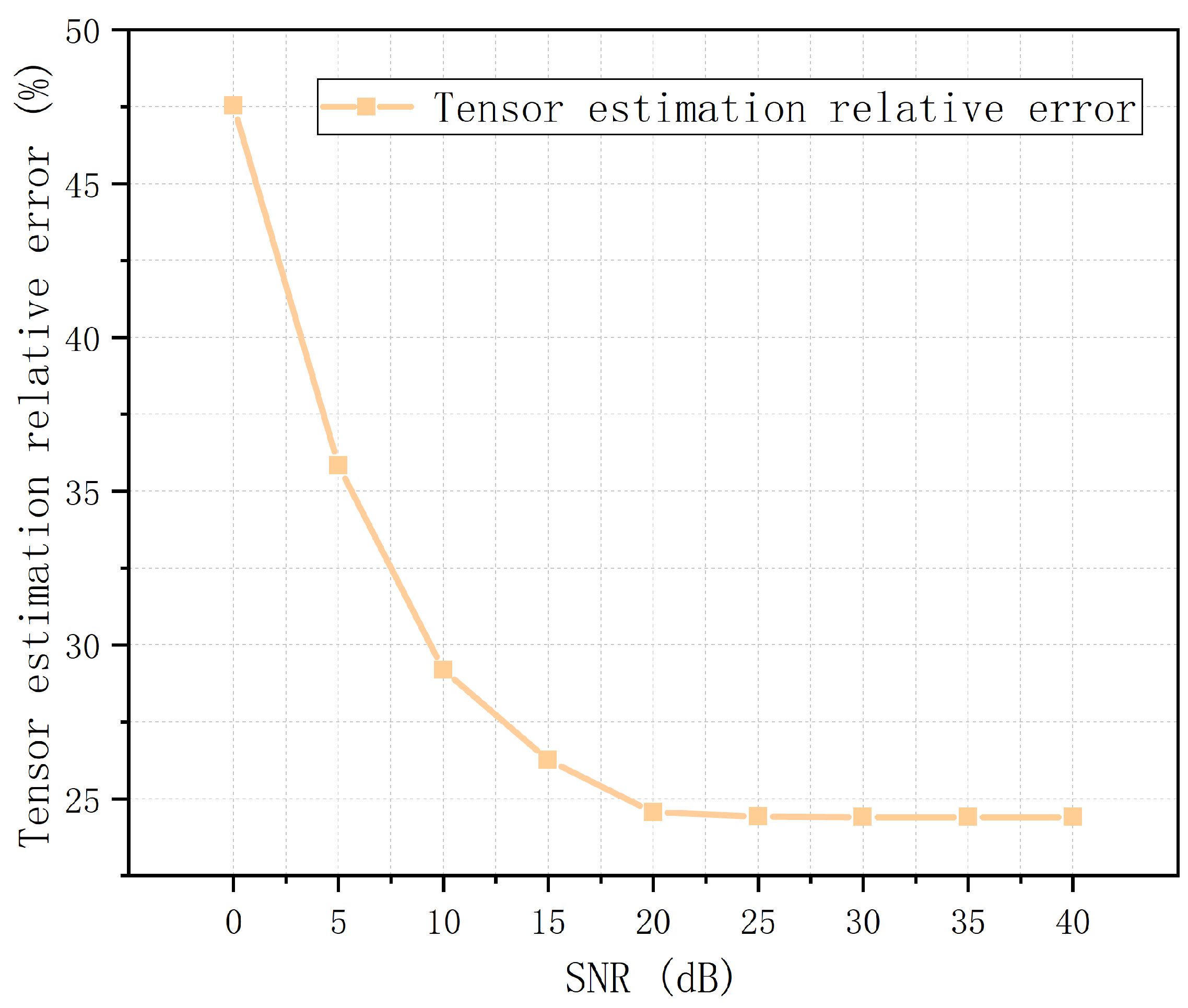
where M ^ 0 i is the estimation of M obtained by using the least squares method in the ith Monte Carlo experiment. The changes in the relative error e ¯ r at different S N R are shown in Figure 11. The changes in e ¯ r are the same as those in d ¯ in Figure 9, which indicate that e ¯ r is related mainly to the depth estimation performance. This result occurs because the horizontal estimation error is much less than the depth estimation error. However, the depth estimation can be kept within an order of magnitude from the true parameter, which is accurate enough for subsequent filter algorithms.

4.2. Target Parameter Estimation Performance

To evaluate the performance of the IVE-KF algorithm, the position estimation error r ¯ , the polarizability estimation error β ¯ e , and the posture angle estimation errors θ ¯ , ϕ ¯ at different simulation conditions are discussed. r ¯ , the values of β ¯ e , θ ¯ and ϕ ¯ for each simulation condition are the average values obtained from 100 Monte Carlo experiments:
r ¯ = i = 1 100 r ^ i r 2 100 ,
β ¯ e = i = 1 100 β ^ i β 2 100 β 2 ,
θ ¯ = i = 1 100 θ i θ ^ i 100 ,
ϕ ¯ = i = 1 100 ϕ i ϕ ^ i 100 ,
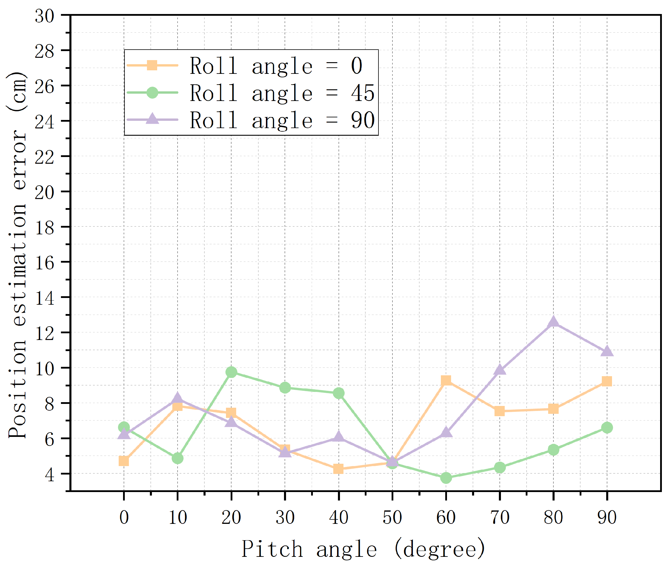
where r ^ i , β ^ i , θ ^ i , ϕ ^ i are respectively the position estimation, polarizability estimation, pitch angle estimation and roll angle estimation obtained by the IVE-KF algorithm at the ith Monte Carlo experiment. r ¯ , β ¯ e , θ ¯ and ϕ ¯ of a cylinder at different postures are shown in Figure 12, Figure 13 and Figure 14. The errors fluctuate as the posture changes, but the position errors are always within 13 cm, the polarization relative errors are within 32 % , and the angle errors are within 10 . When θ = 90 , the phenomenon of gimbal lock [35] occurs, so the angle simulation is performaed only up to 85 .
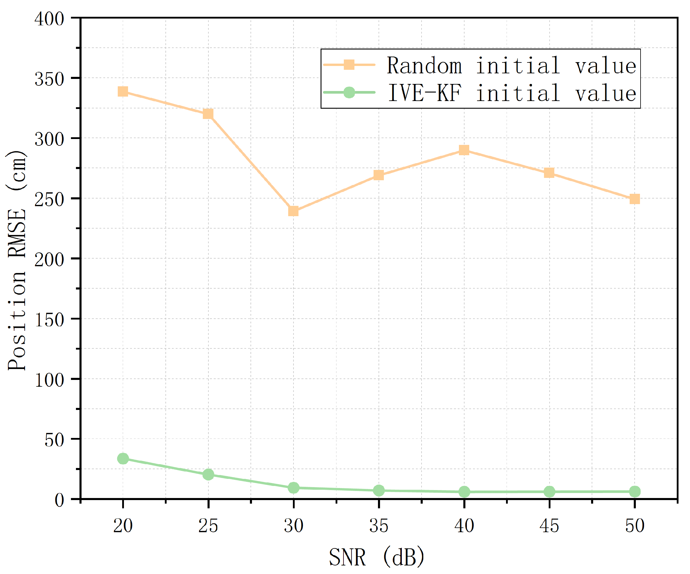
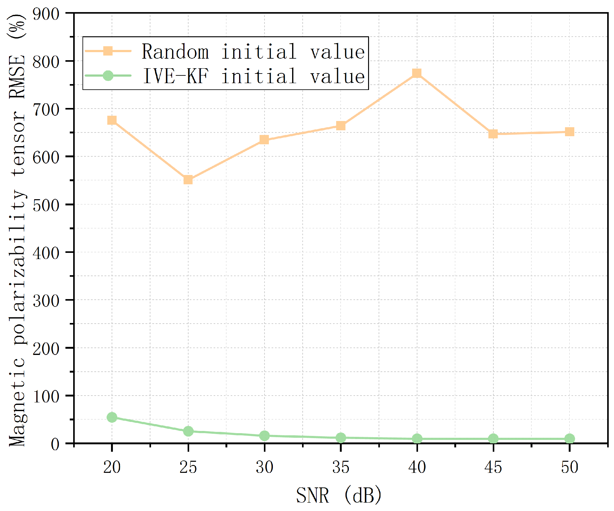
The convergence performances of the IVE-KF algorithm and the filter algorithm with a random initial value are compared in this paper. The convergence results of the algorithm are evaluated using the root mean square error (RMSE) of position and magnetic polarizability tensor.
Figure 15 and Figure 16 show that the filter algorithm with a random initial value cannot converge to the true value at all. Our initial value estimation algorithm provides a relatively accurate initial value for the KF and EKF and improves the convergence and accuracy of the filter algorithm.
The computational complexities of the inversion algorithm and IVE-KF algorithm in this project are also compared. We use the number of floating point operations (FLOPs) to measure the computational complexity of an algorithm. A FLOP is defined as one operation of addition, subtraction, multiplication, or division of two floating point numbers. The FLOPs of the basic algebraic operations are defined in Table 5 [36]:
According to the processes listed in Table 1 and the corresponding Formulas, and assuming that w sets data are collected in the process of detection, the FLOPs of IVE-KF algorithm can be obtained and are shown in Table 6.
The LM algorithm can be analyzed using the same method. The computational complexity of the LM algorithm per iteration is 988 w + 969 FLOPs. The FLOPs comparison of the IVE-KF algorithm and LM algorithm is shown in Table 7:
In Table 7, N i is the iteration times of the LM algorithm. The computational complexity of iterating the LM algorithm twice is equal to the computational complexity of the IVE-KF algorithm. However, the LM algorithm generally iterates 5–8 times in our experiments.
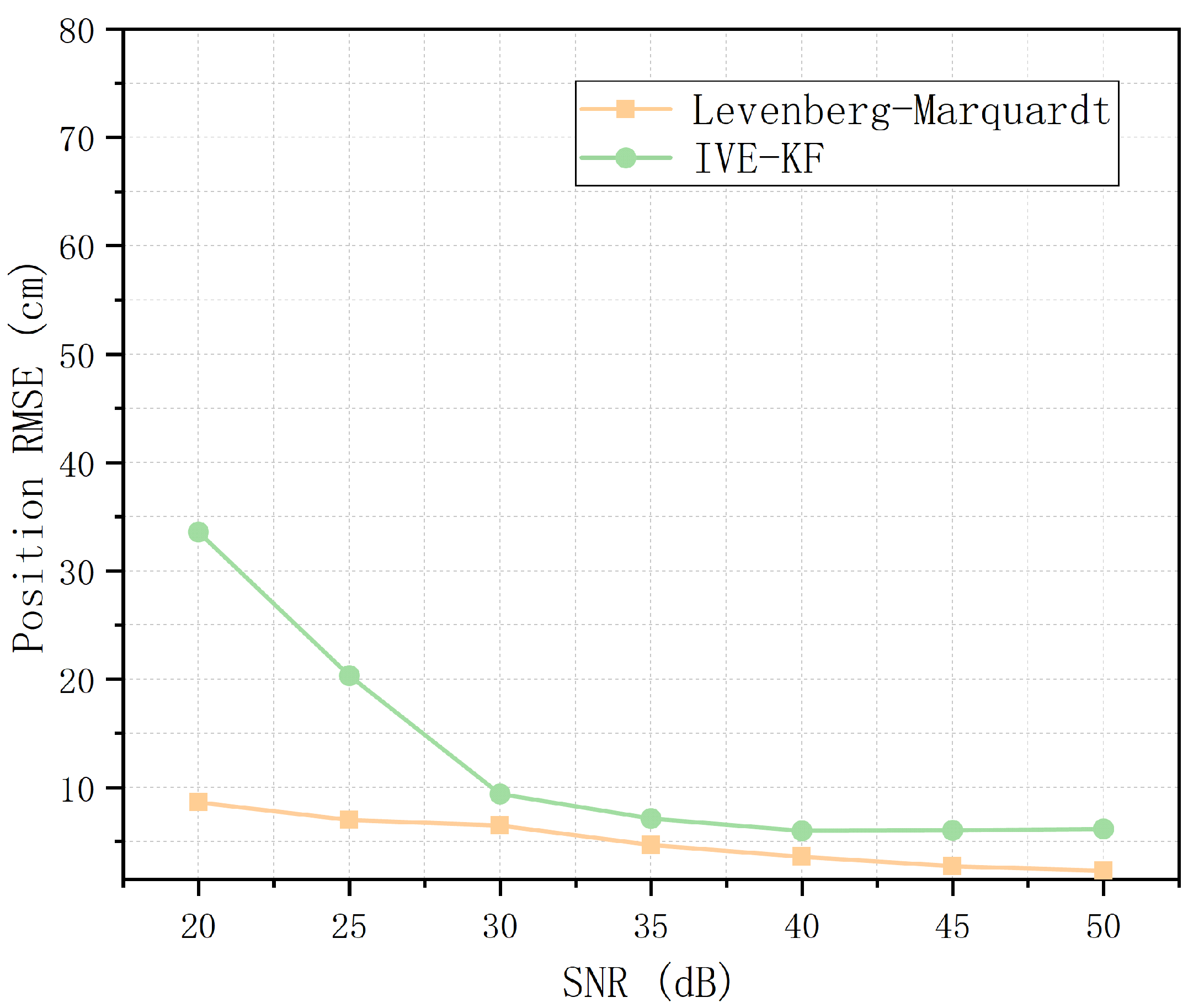
The accuracy performances of the LM algorithm and IVE-KF algorithm are also discussed in terms of the RMSE of the position and magnetic polarizability tensor. Figure 17 and Figure 18 show that the results of the IVE-KF algorithm are not as good as those of the LM algorithm, but the accuracies are very similar when the SNR exceeds 30 dB. This result occurs because of the characteristics of the filter algorithm and inversion algorithm. However, the computational complexity of the LM algorithm is much higher than that of the IVE-KF algorithm. Therefore, future research should focus on the accuracy of the filtering algorithm.

5. Conclusions and Future Work

The traditional filter method in underground metal detection typically receives a fixed or random initial value, resulting in unsatisfactory convergence performance. To improve the convergence performance of the filter algorithm in underground metal detection, the initial value estimation algorithm for the KF and EKF is studied in this paper. To verify the performance of the IVE-KF algorithm, a simulation platform is built. The simulation results show that, in a simulation environment where the detection area is 4 m × 4 m and S N R is 20 dB, the accuracy of the horizontal initial value estimation can be stabilized within 0.5 cm, and the accuracy of depth initial value estimation is stable within 7 cm. The performances of the filter algorithm with a random initial value and the IVE-KF algorithm are compared in this paper. The results show that the convergence of IVE-KF is far better than the convergence of the filter algorithm with a random initial value. The performances of the LM algorithm and IVE-KF algorithm are also compared, and the results show that, when S N R is greater than 30 dB, the detection accuracy of IVE-KF is close to the LM algorithm accuracy. Our method provides a relatively accurate initial value for the filter algorithm in underground metal detection. In future work, we plan to focus on improving the accuracy of the filtering algorithm under low- S N R conditions. On the other hand, our research about underground metal detection is based on the assumption of Gaussian noise distribution. The analysis of the underground metal detection method in non-Gaussian noise is very helpful for practical application. Our next step is to improve the algorithm’s performance in the non-Gaussian noise environment.

Author Contributions

Conceptualization, Y.W. and P.W.; Data curation, Z.W. and Z.L.; Formal analysis, P.W., N.L. and C.Z.; Funding acquisition, Y.W.; Investigation, Z.W. and P.W.; Methodology, P.W., N.L. and C.Z.; Project administration, P.W.; Resources, Y.W.; Software, Z.W. and Z.L.; Supervision, Y.W. and P.W.; Validation, Y.W. and Z.W.; Writing—original draft, Z.W.; Writing—review and editing, P.W.

Funding

This research was funded by the China Postdoctoral Science Foundation under Grant No. 2019M650778, Fundamental Research Funds for the Central Universities under Grant No. 2302018FRF-GF-18-016B and the National Natural Science Foundation of China under Grant No. 61971031.

Acknowledgments

The authors would like to thank all other members of the research team for their contributions to this research.

Conflicts of Interest

The authors declare no conflict of interest.

References

  1. Shubitidze, F.; Barrowes, B.E.; Sigman, J.B.; O’Neill, K.; Shamatava, I. UXO classification procedures applied to advanced EMI sensors and models. In Proceedings of the XXIst International Seminar/Workshop on Direct and Inverse Problems of Electromagnetic and Acoustic Wave Theory (DIPED), Tbilisi, Georgia, 26–29 September 2016; pp. 173–177. [Google Scholar]
  2. Alrumaih, T.N.I. The Construction of a Robotic Vehicle Metal Detector as a Tool for Searching Archaeology Sites. In Proceedings of the 1st International Conference on Computer Applications & Information Security (ICCAIS), Riyadh, Saudi Arabia, 4–6 April 2018; pp. 1–6. [Google Scholar]
  3. Tsukamoto, A.; Hato, T.; Adachi, S.; Motoori, M.; Sugisaki, M.; Tanabe, K. Development of magnetic prospecting system with HTS SQUID gradiometer for exploration of metal resources. In Proceedings of the 15th International Superconductive Electronics Conference (ISEC), Nagoya, Japan, 6–9 July 2015; pp. 1–3. [Google Scholar]
  4. Pham, D.; Aziz, S.M. A real-time localization system for an endoscopic capsule using magnetic sensors. Sensors 2014, 14, 20910–20929. [Google Scholar] [CrossRef] [PubMed]
  5. Guo, Z.Y.; Liu, D.J.; Pan, Q.; Zhang, Y.Y. Forward modeling of total magnetic anomaly over a pseudo-2D underground ferromagnetic pipeline. J. Appl. Geophys. 2015, 113, 14–30. [Google Scholar] [CrossRef]
  6. Grant, F.S.; West, G.F. Interpretation Theory in Applied Geophysics; McGraw-Hill Book Co.: New York, NY, USA, 1965. [Google Scholar]
  7. Grzegorczyk, T.M.; Barrowes, B.E.; Shubitidze, F.; Fernandez, J.P.; O’Neill, K. Simultaneous identification of multiple unexploded ordnance using electromagnetic induction sensors. IEEE Trans. Geosci. Remote Sens. 2011, 49, 2507–2517. [Google Scholar] [CrossRef]
  8. Grzegorczyk, T.M.; Barrowes, B.; Shubitidze, F.; Fernandez, J.; Shamatava, I.; O’Neill, K.A. Kalman filters applied to the detection of unexploded ordnance. In Proceedings of the Detection and Sensing of Mines, Explosive Objects, and Obscured Targets Xv, Orlando, FL, USA, 5–9 April 2010; Volume 7664. [Google Scholar]
  9. Ambruš, D.; Vasić, D.; Bilas, V. Robust estimation of metal target shape using time-domain electromagnetic induction data. IEEE Trans. Instrum. Meas. 2016, 65, 795–807. [Google Scholar] [CrossRef]
  10. Song, L.P.; Oldenburg, D.W.; Pasion, L.R.; Billings, S.D.; Beran, L. Temporal orthogonal projection inversion for EMI sensing of UXO. IEEE Trans. Geosci. Remote Sens. 2015, 53, 1061–1072. [Google Scholar] [CrossRef]
  11. Abedi, M.; Mosazadeh, K.; Dehghani, H.; MADANCHI, Z.A. Geological noise removal in geophysical magnetic survey to detect unexploded ordnance based on image filtering. Iran. Geophys. 2016, 9, 11–23. [Google Scholar]
  12. Sadatcharam, K. Assessing Potential Applications of Multi-Coil and Multi-Frequency Electromagnetic Induction Sensors for Agricultural Soils in Western Newfoundland. Ph.D. Thesis, Memorial University of Newfoundland, St. John’s, NL, Canada, 2019. [Google Scholar]
  13. Grzegorczyk, T.M.; Barrowes, B.E. Real-time processing of electromagnetic induction dynamic data using Kalman filters for unexploded ordnance detection. IEEE Trans. Geosci. Remote Sens. 2012, 51, 3439–3451. [Google Scholar] [CrossRef]
  14. Wang, H.; Chen, S.; Zhang, S.; Yuan, Z.; Zhang, H.; Fang, D.; Zhu, J. A high-performance portable transient electro-magnetic sensor for unexploded ordnance detection. Sensors 2017, 17, 2651. [Google Scholar] [CrossRef]
  15. Dekdouk, B.; Marsh, L.A.; Armitage, D.W.; Peyton, A.J. Estimating magnetic polarizability tensor of buried metallic targets for land mine clearance. In Ultra-Wideband, Short-Pulse Electromagnetics 10; Springer: Berlin/Heidelberg, Germany, 2014; pp. 425–432. [Google Scholar]
  16. Ambruš, D.; Vasić, D.; Bilas, V. Characterization of buried targets from planar electromagnetic induction sensor data in a moving reference frame. Int. Soc. Opt. Photonics 2017, 10182, 1018215. [Google Scholar]
  17. Chan, Y.; Hu, A.; Plant, J. A Kalman filter based tracking scheme with input estimation. IEEE Trans. Aerosp. Electron. Syst. 1979, 15, 237–244. [Google Scholar] [CrossRef]
  18. Koopman, S.J. Exact initial Kalman filtering and smoothing for nonstationary time series models. J. Am. Stat. Assoc. 1997, 92, 1630–1638. [Google Scholar] [CrossRef]
  19. Grzegorczyk, T.M.; Barrowes, B.; Shubitidze, F.; Fernandez, J.; Shamatava, I.; O’Neill, K.A. Kalman filters applied to the detection of unexploded ordnance. Int. Soc. Opt. Photonics 2010, 7664, 766402. [Google Scholar]
  20. Tantum, S.L.; Collins, L.M. Detection and classification of land-mine-like targets in a non-Gaussian noise environment. Int. Soc. Opt. Photonics 2000, 4038, 900–909. [Google Scholar]
  21. Gordon, N.J.; Salmond, D.J.; Smith, A.F. Novel approach to nonlinear/non-Gaussian Bayesian state estimation. Radar Signal Process. 1993, 140, 107–113. [Google Scholar] [CrossRef] [Green Version]
  22. Jay, E.; Ovarlez, J.P.; Declercq, D.; Duvaut, P. Bayesian optimum radar detector in non-Gaussian noise. In Proceedings of the IEEE International Conference on Acoustics, Speech, and Signal Processing, Orlando, FL, USA, 13–17 May 2002. [Google Scholar]
  23. Qu, X.; Li, Y.; Fang, G.; Yin, H. A portable frequency domain electromagnetic system for shallow metal targets detection. Prog. Electromagn. Res. 2017, 53, 167–175. [Google Scholar] [CrossRef]
  24. Xiaodong, Q.; Chen, W.; Guangyou, F.; Hejun, Y. Detecting anomaly targets using handheld frequency domain electromagnetic system. Sens. Actuators 2017, 268, 155–163. [Google Scholar] [CrossRef]
  25. Stutzman, W.L.; Thiele, G.A. Antenna Theory and Design; John Wiley & Sons: Hoboken, NJ, USA, 2012. [Google Scholar]
  26. Shubitidze, F. A Complex Approach to UXO Discrimination: Combining Advanced EMI Forward MODELS and Statistical Signal Processing; Technical Report; Sky Research Inc.: Ashland, OR, USA, 2012. [Google Scholar]
  27. Arfken, G.B.; Weber, H.J. Mathematical Methods for Physicists; Academic Press: Cambridge, MA, USA, 1999. [Google Scholar]
  28. Abdel-Rehim, O.A.; Davidson, J.L.; Marsh, L.A.; O’Toole, M.D.; Peyton, A.J. Magnetic polarizability tensor spectroscopy for low metal anti-personnel mine surrogates. IEEE Sens. J. 2016, 16, 3775–3783. [Google Scholar] [CrossRef]
  29. Pasion, L.R. Detecting Unexploded Ordnance with Time Domain Electromagnetic Induction. Ph.D. Thesis, University of British Columbia, Vancouver, BC, Canada, 1999. [Google Scholar]
  30. Hu, M.K. Visual pattern recognition by moment invariants. IRE Trans. Inf. Theory 1962, 8, 179–187. [Google Scholar]
  31. Pasion, L.R.; Oldenburg, D.W. Locating and Characterizing Unexploded Ordnance Using Time Domain Electromagnetic Induction; Technical Report; British Columbia University: Vancouver, BC, Canada, 2001. [Google Scholar]
  32. Neumaier, A. Solving ill-conditioned and singular linear systems: A tutorial on regularization. SIAM Rev. 1998, 40, 636–666. [Google Scholar] [CrossRef]
  33. Golub, G.H.; Hansen, P.C.; O’Leary, D.P. Tikhonov regularization and total least squares. SIAM J. Matrix Anal. Appl. 1999, 21, 185–194. [Google Scholar] [CrossRef]
  34. Bell, T.; Barrow, B.; Miller, J.; Keiswetter, D. Time and frequency domain electromagnetic induction signatures of unexploded ordnance. Subsurf. Sens. Technol. Appl. 2001, 2, 153–175. [Google Scholar] [CrossRef]
  35. Strickland, J. What Is a Gimbal—And What Does It Have to Do with NASA. Available online: https://science.howstuffworks.com/gimbal.htm (accessed on 20 September 2019).
  36. Grewal, M.S.; Andrews, A.P.; Bass, R. Kalman filtering: Theory and practice. IEEE Trans. Autom. Control 1995, 40, 1983. [Google Scholar]
Figure 1. Process of the metal detection system.
Applsci 09 04113 g001
Figure 2. Primary field model in spherical coordinates.
Applsci 09 04113 g002
Figure 3. Diagram of electromagnetic induction (EMI) detection.
Applsci 09 04113 g003
Figure 4. Secondary field spatial response of spherical and cylindrical objects. (a) shows detection scenes, and the red lines and small circles denote the track of the detector; (b) shows the secondary field strength map of (a).
Applsci 09 04113 g004
Figure 5. EMI simulation system diagram.
Applsci 09 04113 g005
Figure 6. Cylinder in the detection system.
Applsci 09 04113 g006
Figure 7. The secondary field strength map of a cylindrical target ( θ = 9 0 ). (a) the component B x of the secondary field in the x-axis direction; (b) the component B y of the secondary field in the y-axis direction; (c) the component B z of the secondary field in the z-axis direction; (d) total secondary field B s .
Applsci 09 04113 g007
Figure 8. Estimation error of the horizontal position of the cylindrical target at different signal-to-noise ratio (SNR) values.
Applsci 09 04113 g008
Figure 9. Cylindrical target depth estimation error at different SNR values.
Applsci 09 04113 g009
Figure 10. Depth estimation error of a cylindrical target at different depths.
Applsci 09 04113 g010
Figure 11. Estimation error of the magnetic polarizability tensor element of a cylindrical target at different SNR values.
Applsci 09 04113 g011
Figure 12. Position error accuracy of the initial value estimation method for the Kalman filter (KF) and the extend Kalman filter (EKF) (IVE-KF) algorithm at different posture angles.
Applsci 09 04113 g012
Figure 13. Error of the polarizability error of the IVE-KF algorithm at different posture angles.
Applsci 09 04113 g013
Figure 14. Posture error accuracy of the IVE-KF algorithm at different posture angles.
Applsci 09 04113 g014
Figure 15. Root mean square error (RMSE) comparison of the position error between the IVE-KF algorithm and filter algorithm given random initial values.
Applsci 09 04113 g015
Figure 16. RMSE comparison of the magnetic polarizability tensor errors between the IVE-KF algorithm and filter algorithm given random initial values.
Applsci 09 04113 g016
Figure 17. RMSE comparison of the position error between the inversion algorithm and filter algorithm.
Applsci 09 04113 g017
Figure 18. RMSE comparison of the magnetic polarizability tensor error of the inversion algorithm and filter algorithm.
Applsci 09 04113 g018
Table 1. Initial value estimation method for the Kalman filter (KF) and the extend Kalman filter (EKF) (IVE-KF) algorithm iteration process.
Input: collected data C 1 : w , detector position r d 1 : w
- Initial value estimation: r ^ 0 is calculated according to Formulas (17) and (18), and  M ^ 0 is calculated according to Formula (26)
- Traverse each detector position r d k
KF: Recursively update M ^
   - Calculate the Green function G r d k r ^ according to Formula (5)
   - Calculate the primary field B p r ^ r d k according to Formulas (1)–(3)
   - Calculate W k according to Formulas (21) and (22)
   - Update M ^ according to Formulas (31) and (32)
EKF: Recursively update r ^
   - Calculate the Jacobian matrix H k r = r ^ according to Formulas (34) and (37)
   - Update r ^ according to Formulas (35) and (36)
- End
Output: α ^ = r ^ T , M ^ T T
Table 2. Transmitter simulation parameters and default values.
Parameter NameSymbolDefault Value
Coil radiusa0.5 m
Peak of the harmonic current I 0 20 A
Angular frequency ω 1000 Hz
Table 3. Detected target simulation parameters and default values.
Parameter NameSymbolDefault Value
Position vector r 0 , 0 , 4 m
Radius a s 0.2 m
Height (cylindrical targets only)L1.0 m
Conductivity σ 5 . 17 × 10 7 ; (S/m)
Relative permeability μ r 1
Yaw angle ψ 0
Pitch angle θ 0
Roll angle ϕ 0
Table 4. Data collection simulation parameters and default values.
Parameter NameSymbolDefault Value
Line interval l s 0.1 m
Point interval p s 0.1 m
Number of scanning lines 2 M + 1 41
Sampling points of each scanning line 2 N + 1 41
Signal to noise ratio S N R 20 dB
Table 5. Floating point operations (FLOPs) of basic algebraic operations.
OperationSymbolDescriptionFLOPs
Matrix addition A + B A R n × m , B R n × m n m
Matrix subtraction A B A R n × m , B R n × m n m
Matrix multiplication A B A R n × m , B R m × l 2 n m l n l
Matrix inversion A 1 A R n × n n 3
Table 6. FLOPs of IVE-KF algorithm.
OperationFLOPs
Estimating the initial value 324 w + 360
Calculating the Green function 27 w
Calculating the primary field 31 w
KF algorithm 1161 w
EKF algorithm 738 w
Total 2281 w + 360
Table 7. Comparison of FLOPs.
AlgorithmFLOPs
IVE-KF 2281 w + 360
Levenberg–Marquardt (LM) N i ( 988 w + 969 )