Air Quality Index and Air Pollutant Concentration Prediction Based on Machine Learning Algorithms

Abstract

Air pollution has become an important environmental issue in recent decades. Forecasts of air quality play an important role in warning people about and controlling air pollution. We used support vector regression (SVR) and random forest regression (RFR) to build regression models for predicting the Air Quality Index (AQI) in Beijing and the nitrogen oxides (NO_X) concentration in an Italian city, based on two publicly available datasets. The root-mean-square error (RMSE), correlation coefficient (r), and coefficient of determination (R²) were used to evaluate the performance of the regression models. Experimental results showed that the SVR-based model performed better in the prediction of the AQI (RMSE = 7.666, R² = 0.9776, and r = 0.9887), and the RFR-based model performed better in the prediction of the NO_X concentration (RMSE = 83.6716, R² = 0.8401, and r = 0.9180). This work also illustrates that combining machine learning with air quality prediction is an efficient and convenient way to solve some related environment problems.

1. Introduction

Many environmental crises currently confront us: global warming, hazardous waste, resource depletion, air pollution, and many more [1,2,3,4]. Millions of people die every year from diseases caused by exposure to outdoor air pollution [5]. In China, the health risk from overexposure to particles is becoming an important public health concern [6]. China’s capital, Beijing, has experienced rapid development in economy and energy consumption. Along with this rapid development, hazy weather caused by air pollution has become increasingly serious in Beijing. Air-pollution-weather occurs often and lasts for a long time, although it has seemed better in the last two years [7].

The Air Quality Index (AQI) is an important indicator to reflect and evaluate air quality [8]. According to the Chinese Standard GB3095-2012 [9], AQI is calculated by six major pollutants: fine particulate matter (PM_2.5), ozone (O₃), sulfur dioxides (SO₂), inhalable particles (PM₁₀), nitrogen dioxides (NO₂), and carbon monoxide (CO) [10]. The AQI measures the overall quality of the air on a scale with a range of 0 to 500 that is divided into six levels (good, moderate, lightly polluted, moderately polluted, heavily polluted, and severely polluted); these levels show the impact on human health and provide a good reference for people’s outdoor activities in a numerical form [11]. A low number means good air quality, while a higher number means worse air quality, which has ramifications for people’s outdoor activities.

Governing and solving air pollution problems is a long-term process. Air quality forecasting can help with the prevention of damage caused by air pollution. Therefore, it is necessary for air quality forecasting to occur in a timely manner, to allow government departments and the public to take protective measures and prevent serious pollution incidents. For instance, some plants in Beijing, such as coal-fired power plants and coking plants, have shut down temporarily as a result of the predicted air quality [12].

Machine learning is the scientific study of algorithms and statistical models that computer systems use to make predictions or decisions without being explicitly programmed to perform the task [13]. Machine learning has gained tremendous popularity for its powerful and fast predictions with big data [14]. Big data means enormous datasets, including masses of unstructured data that need more real-time analysis to help us to gain an in-depth understanding of its hidden values [15].

Some researchers have applied machine learning algorithms to the short- and long-term prediction of air quality successfully [16,17,18,19]. Pérez et al. predicted the hourly concentration of PM_2.5 in Santiago using a multilayer neural network [20]. Focusing on the problem of poor prediction, authors have discussed using a larger dataset for improvements. Zhu et al. proposed two hybrid models (empirical mode decomposition (EMD)–support vector regression (SVR) hybrid and EMD–intrinsic mode functions (IMF) hybrid) to forecast AQI in Xingtai, with the EMD–SVR hybrid model achieving a highest overall accuracy of 80% [11]. However, in the experiment, the authors used only a single indicator (past AQI data) to predict the present AQI, and ignored the correlation between different pollutants (such as PM_2.5, PM₁₀, and so on). Corani et al. used feed-forward neural networks to predict ozone and PM₁₀ in Milan [21]. Although the predictions showed a satisfactory reliability, the model still has the tendency toward overfitting, as the authors reported. Biancofiore et al. used a recursive neural network model to forecast PM₁₀ concentration 1, 2, and 3 days ahead [22]. The recursive neural network model forecasted correctly 95% of the days. However, the percentage of false positives was 30%, which highlights the limits of the neural network model in simulating concentration peaks. Fuller et al. devised an empirical model to predict concentrations of PM₁₀ at background and roadside locations in London [23]. However, the performance of the model relied heavily on the currently observed ratio between NO_X and PM₁₀.

Motivated by prior studies, we first explored the correlation of various air indicators, such as the AQI, the concentration of PM_2.5, the concentration of total nitrogen oxides (NO_X), and so on. Second, we used support vector regression (SVR) and random forest regression (RFR) to build prediction models. Finally, we used RMSE, correlation coefficient r, and coefficient of determination R² to evaluate the performance of the regression models.

The rest of this paper is organized as follows. Details about the datasets and pattern recognition methods (SVR and RFR) are briefly reviewed in Section 2. Section 3 shows the results of the models’ prediction, along with corresponding discussion. Conclusions are drawn in Section 4.

2. Materials and Methods

2.1. Area of Investigation and Datasets

In this study, two publicly available datasets were used.

The first dataset, the Beijing Air Quality Dataset (December 2013 to August 2018), is from the Beijing Municipal Environmental Monitoring Center [24]. The dataset has 1738 instances. Each instance consists of hourly averaged AQI and the concentrations for PM_2.5, O₃, SO₂, PM₁₀, and NO₂ in Beijing, provided by an officially certified analyzer.

The second dataset comes from an air quality recording that contains the responses of a gas multi-sensor device deployed on a field in an Italian city. The dataset [3,25,26] contains 9358 instances of hourly averaged responses from an array of five metal oxide chemical sensors embedded in an air quality chemical multi-sensor device. Data were recorded from March 2004 to February 2005 (one year), representing the longest freely available recordings of an air quality chemical sensor device deployed in the field. Hourly averaged concentrations for CO, non-methane hydrocarbons, benzene, NO_X, and NO₂ were provided by a co-located reference certified analyzer. Missing values are tagged with −200 value. For the purposes of this study, we focus on NO_X prediction, using the second dataset. As we know, NO_X is another important indicator for air quality evaluation. NO_X emissions have been linked to acid rain, photochemical smog, and tropospheric ozone destruction [27]. Moreover, when nitrogen oxides are inhaled by the human body, they disrupt the alveolar structures and their function in lungs, posing a great threat to human health [28].

2.2. Pattern Recognition Methods

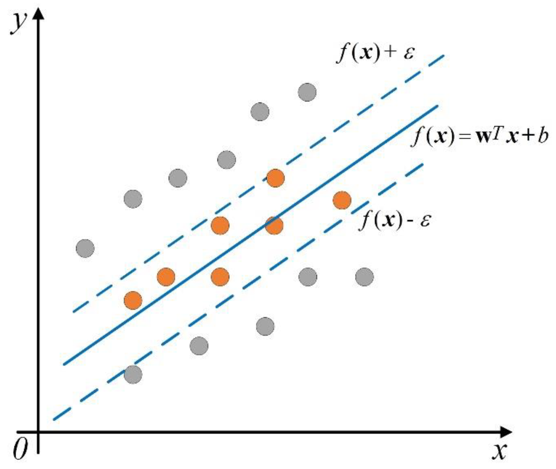
2.2.1. Support Vector Machines (SVMs)

Support vector machines (SVMs) are supervised learning models, with associated learning algorithms that analyze the data used for classification and regression analyses [29,30].

A type of SVM for regression, support vector regression (SVR), was originally proposed by Vapnik and his coworkers [28]. In SVR, the set of training data includes predictor variables and observed response values. The goal is to find a function f(x) that deviates from y_n (sample labels) by a value no greater than ε (bias) for each training point x—that is, remain as flat as possible. Therefore, SVR is also known as tube regression. Its schematic diagram is shown in Figure 1.

According to the literature on SVM linear regression [28], the solution to SVR is as follows:

$$f(\mathit{x})={\displaystyle \sum _{n=1}^N(a_n-a_n^{*})}({\mathit{x}}_n^{\mathrm{T}}\mathit{x})+b.$$

(1)

Where x is the input feature vector, b is the distance parameter, $a_n$ and $a_n^{*}$ are the introduced Lagrange multipliers. However, some regression problems cannot be described adequately using a linear model. In that case, we can obtain a nonlinear SVR model by replacing the dot product ${\mathit{x}}_n^{\mathrm{T}}\mathit{x}$ with a nonlinear kernel function K(x₁, x₂) = <φ(x₁), φ(x₂)>, where φ(x) is a transformation that maps x to a high-dimensional space. Therefore, the final solution to nonlinear SVR can be obtained as:

$$f(\mathit{x})={\displaystyle \sum _{n=1}^N(a_n-a_n^{*})}K(\mathit{x},{\mathit{x}}_n)+b.$$

(2)

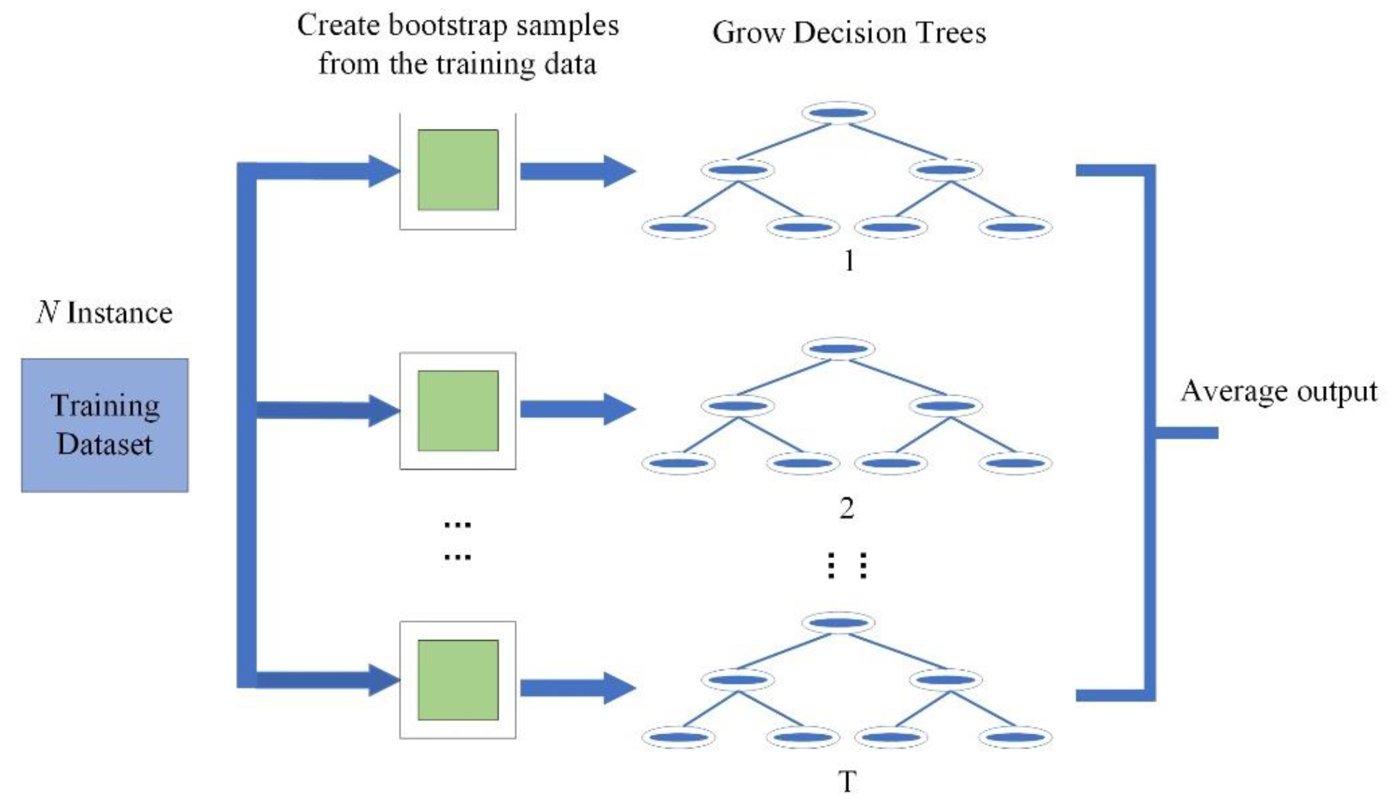
2.2.2. Random Forest (RF)

Random forests (RFs), or random decision forests, are an ensemble learning method for classification, regression, and other tasks. An RF operates by constructing multiple decision trees at different training times, and outputting the class representing the mode of classes (classification) or the mean prediction (regression) of individual trees [31].

The RF algorithm incorporates growing classification and regression trees (CARTs). Each CART is built using random vectors. For the RF-based classifier model, the main parameters were the number of decision trees, as well as the number of features (N_F) in the random subset at each node in the growing trees. During model training, the number of decision trees was determined first. For the number of trees, a larger number is better, but takes longer to compute. A lower N_F leads to a greater reduction in variance, but a larger increase in bias. N_F can be defined using the empirical formula $N_F=\sqrt{M}$, where M denotes the total number of features [32].

RF can be applied to classification and regression problems, depending on whether the trees are classification or regression trees. The regression model is shown in Figure 2. Assuming that the model includes T regression trees (learners) for regression prediction, the final output of the regression model is

$$H(\mathit{x})=\frac{1}{T}{\displaystyle \sum _{i=1}^T{\mathrm{h}}_{\mathrm{i}}(\mathit{x})},$$

(3)

where T is the number of regression trees, and h_i(x) is the output of the i-th regression tree (h_i) on sample x. Therefore, the prediction of the RF is the average of the predicted values of all the trees.

3. Results and Discussion

In this work, SVR and RFs were used to build prediction models for the AQI of Beijing and the NO_X of an Italian city, respectively.

RMSE, r, and R² were used to evaluate the performance of the regression models. To obtain a good regression model, the following criteria could be used as references: (1) low RMSE, (2) high r, and (3) high R². The mathematical expressions of the parameters are shown in Equations (4)–(6), where $y_i$ is the label of the i-th sample, $\widehat{y_i}$ is the predicted value of the i-th sample, and the superscript horizontal line indicates the average value. RMSE represents the sample’s standard deviation of the differences between the predicted values and the observed values. The correlation coefficient (r) is a number that quantifies the type of correlation and dependence, implying the statistical relationships between two or more values in fundamental statistics. The coefficient of determination (R²) is proportional to the variance in the dependent variable that is predictable from the independent variable(s) [33].

$$\mathrm{RMSE}=\sqrt{\frac{1}{n}{\displaystyle \sum _{i=1}^n{(\widehat{y_i}-y_i)}^2}}$$

(4)

$$\mathrm{r}=\frac{{\displaystyle \sum _{i=1}^n(y_i-\overline{y})(\widehat{y_i}-\overline{\widehat{y}})}}{\sqrt{{{\displaystyle \sum _{i=1}^n(y_i-\overline{y})}}^2}\sqrt{{{\displaystyle \sum _{i=1}^n(\widehat{y_i}-\overline{\widehat{y}})}}^2}}$$

(5)

$${\mathrm{R}}^2=1-\frac{{\displaystyle \sum _i^n{(y_i-\widehat{y_i})}^2}}{{\displaystyle \sum _i^n{(y_i-\overline{y})}^2}}$$

(6)

We know that the AQI and the concentration of air pollutants (CAP) are affected by many factors. In particular, when gas diffusion conditions are poor, the concentration of various pollutants increases, so there are correlations between the concentration of each pollutant. Before the regression model was established, we studied the correlation of various indicators.

Figure 3a,b shows the correlation between the 6 and 11 air pollution indicators, respectively; we found that these indicators are highly correlated. Therefore, when one or more indicators is missing, it is feasible to use the remaining indicators to predict missing indicators. Taking the AQI prediction and NO_X concentration prediction as examples, we constructed a regression model to verify the feasibility of our proposed method.

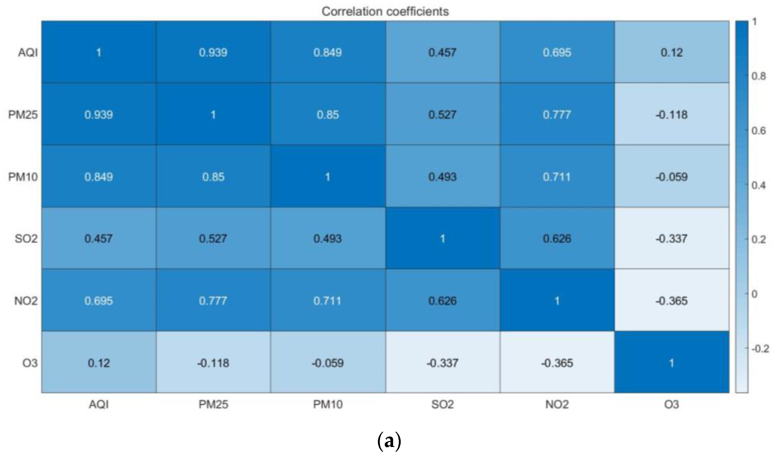
3.1. Air Quality Index Prediction of Beijing

In this experiment, we took the AQI of Beijing as the regression target. The data from the first four years of the dataset were used to train the model, and the data from the last year were used for the model testing.

For the SVR-based model training, radial basis function (RBF) was chosen as the kernel function. The kernel parameter gamma (γ) and the penalty parameter (C) were selected by a grid search method. The experimental results showed that the best combination for the SVR model was C = 10 and γ = 0.1.

Table 1. The statistical parameters of the experiments for the Air Quality Index (AQI) and total nitrogen oxide (NO_X) prediction.

Algorithm	Result of AQI Prediction			Result of NOX Prediction
	r	R2	RMSE	r	R2	RMSE
SVR	0.9887	0.9766	7.666	0.8923	0.7960	94.4918
RFR	0.9823	0.9633	9.602	0.9180	0.8401	83.6716

summarizes the statistical parameters of the SVR regression model for AQI prediction. The statistical parameters for the testing set were as follows: r = 0.9887, R² = 0.9776, and RMSE = 7.666. These results demonstrate that the SVR-based method was a good substitute for analyzing the regression on the AQI.

In this experiment, for the RF-based model, 100 regression trees were used to build the regression model; N_F was defined using the empirical formula ($N_F=\sqrt{M}$) mentioned earlier. The statistical parameters (r = 0.9823, R² = 0.9633, and RMSE = 9.602) of the RFR-based model are also shown in Table 1.

As shown in Figure 4, the AQI of the testing samples was estimated using SVR and RFR, with the x-axis denoting the sequence number of the testing samples and the y-axis (target value) representing the AQI of Beijing. Subplots 4a and 4b, the line chart of the actual values, and the values predicted using different regression models, all reflect the regression of the AQI very well. In particular, the SVR-based model shows better performance.

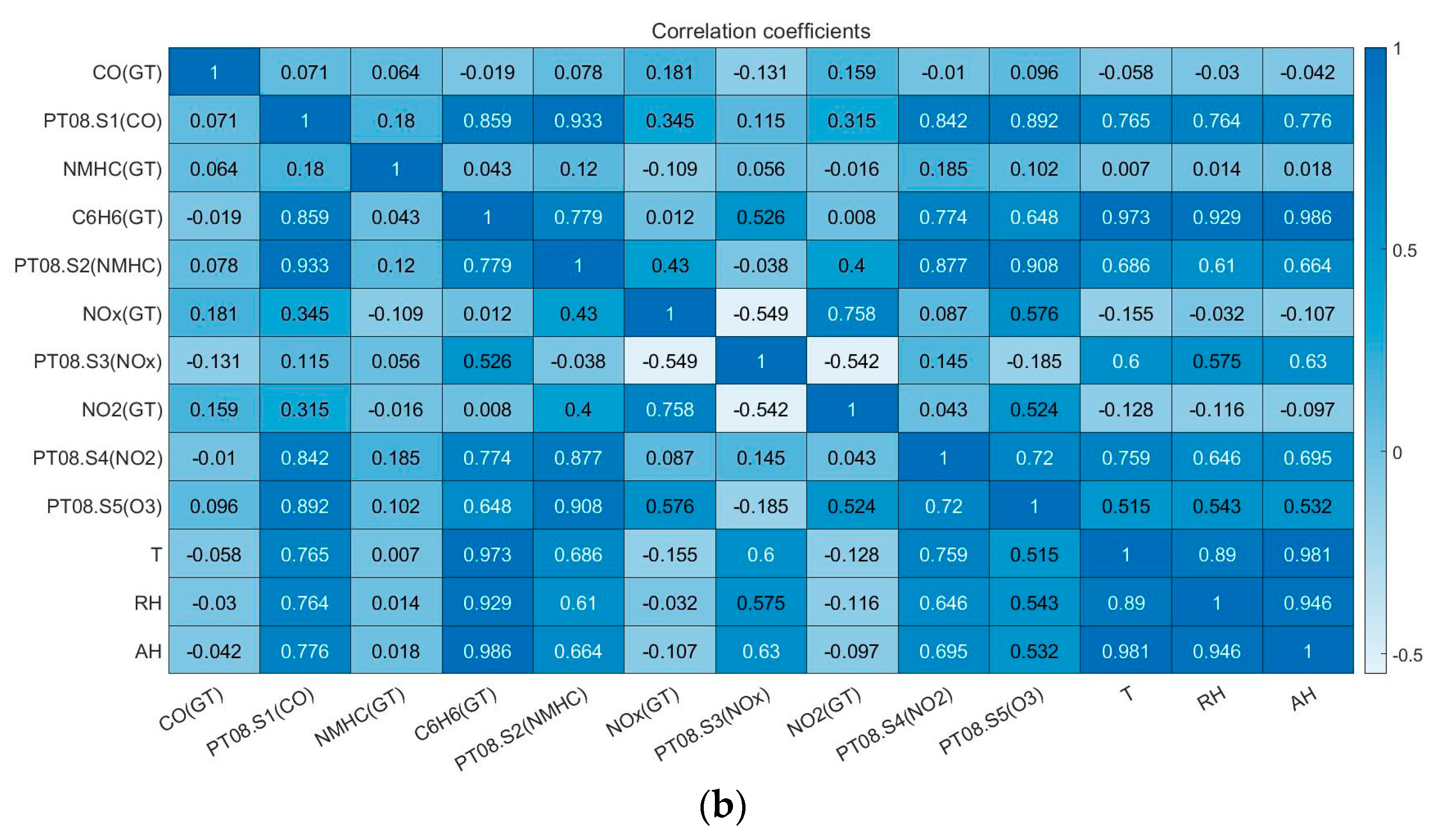
3.2. NO_X Prediction in an Italian City

In this experiment, we took the NO_X concentration of an Italian city as the regression target. Data from the last three months were used to test the model, and the remaining data were used for the model training.

For the SVR-based model training, RBF was also chosen as the kernel function. The kernel parameter gamma (γ) and the penalty parameter (C) were also selected by a grid search method. The experimental results showed that the best combination for the SVR model was C = 20 and γ = 0.15. Table 1 summarizes the statistical parameters of the SVR regression model for the AQI prediction. In the testing set, the statistical parameters were as follows: r = 0.8923, R² = 0.7960, and RMSE = 94.4918.

For the RF-based model in our experiment, we also used 100 regression trees to build the regression model. The model achieved the criteria for good performance, with r = 0.9180, R² = 0.8401, and RMSE = 83.6716, which is also shown in Table 1. The results showed that the RFR-based method was a better substitute for analyzing the regression on the NO_X.

As shown in Figure 5, the NOx of the testing samples was estimated using SVR and RFR, with the x-axis denoting the sequence number of the testing samples and the y-axis (target value) representing the NO_X of the Italian city. In Figure 5, the line chart of the actual values and the values predicted using different regression models demonstrates that the regression model based on RFR is a better predictor than the model based on SVR.

4. Conclusions

Accurate air quality forecasting has important theoretical and practical value for the public; without it, neither the government nor the public can effectively avoid the health damage caused by air pollution or improve the emergency response capability of heavy pollution days. In this study, we built regression models to predict air indicators based on machine learning algorithms, taking the AQI prediction of Beijing and the pollutant concentration prediction of an Italian city as examples. The experimental results show that both the SVR-based model and the RFR-based model can achieve good results, but the RFR model performs better in experiments. In addition, with the increasing number of samples, the time complexity of the SVR model increased cubically. Therefore, the SVR model is not suitable for processing a large number of samples. In summary, this study established two prediction models based on different prediction scenarios, which improved the prediction accuracy of air indicators and provides guidance for modeling and analyzing urban air quality.

References

1. Vitousek, P.M. Beyond global warming: Ecology and global change. Ecology 1994, 75, 1861–1876. [Google Scholar] [CrossRef]
2. Yilmaz, O.; Kara, B.Y.; Yetis, U. Hazardous waste management system design under population and environmental impact considerations. J. Environ. Manag. 2017, 203, 720–731. [Google Scholar] [CrossRef] [PubMed] [Green Version]
3. De Vito, S.; Piga, M.; Martinotto, L.; Di Francia, G. CO, NO2 and NOX urban pollution monitoring with on-field calibrated electronic nose by automatic bayesian regularization. Sens. Actuators B 2009, 143, 182–191. [Google Scholar] [CrossRef]
4. Northey, S.A.; Mudd, G.M.; Werner, T.T. Unresolved complexity in assessments of mineral resource depletion and availability. Nat. Resour. Res. 2018, 27, 241–255. [Google Scholar] [CrossRef]
5. Zhang, Q.; Jiang, X.; Tong, D.; Davis, S.J.; Zhao, H.; Geng, G.; Feng, T.; Zhang, B.; Lu, Z.; Streets, D.G.; et al. Transboundary health impacts of transported global air pollution and international trade. Nature 2017, 543, 705. [Google Scholar] [CrossRef] [PubMed]
6. Du, X.A.; Kong, Q.A.; Ge, W.H.; Zhang, S.J.; Fu, L.X. Characterization of personal exposure concentration of fine particles for adults and children exposed to high ambient concentrations in Beijing, China. J. Environ. Sci. China 2010, 22, 1757–1764. [Google Scholar] [CrossRef]
7. Annual Average Concentration of Air Pollutants of Beijing, China in 2018 (in Micrograms per Cubic Meter). Available online: https://www.statista.com/statistics/1042215/china-average-concentration-of-air-pollutants-in-beijing/ (accessed on 24 September 2019).
8. Kyrkilis, G.; Chaloulakou, A.; Kassomenos, P.A. Development of an aggregate Air Quality Index for an urban Mediterranean agglomeration: Relation to potential health effects. Environ. Int. 2007, 33, 670–676. [Google Scholar] [CrossRef]
9. China Ministry of Environmental Protection. Ambient Air Quality Standards. GB 3095-2012; China Environmental Science Press: Beijing, China, 2012. [Google Scholar]
10. Sheng, N.; Tang, U.W. The first official city ranking by air quality in China—A review and analysis. Cities 2016, 51, 139–149. [Google Scholar] [CrossRef]
11. Zhu, S.; Lian, X.; Liu, H.; Hu, J.; Wang, Y.; Che, J. Daily air quality index forecasting with hybrid models: A case in China. Environ. Pollut. 2017, 231, 1232–1244. [Google Scholar] [CrossRef]
12. Zhang, H.; Wang, S.; Hao, J.; Wang, X.; Wang, S.; Chai, F.; Li, M. Air pollution and control action in Beijing. J. Clean. Prod. 2016, 112, 1519–1527. [Google Scholar] [CrossRef]
13. Bishop, C.M. Pattern Recognition and Machine Learning; Springer: New York, NY, USA, 2006. [Google Scholar]
14. Machine Learning Algorithms. Available online: https://www.packtpub.com/big-data-and-business-intelligence/machine-learning-algorithms-second-edition (accessed on 9 September 2019).
15. Chen, M.; Mao, S.; Liu, Y. Big data: A survey. Mob. Netw. Appl. 2014, 19, 171–209. [Google Scholar] [CrossRef]
16. Cabaneros, S.M.S.; Calautit, J.K.S.; Hughes, B.R. A review of artificial neural network models for ambient air pollution prediction. Environ. Model. Softw. 2019, 119, 285–304. [Google Scholar] [CrossRef]
17. Cabaneros, S.M.S.; Calautit, J.K.S.; Hughes, B.R. Hybrid artificial neural network models for effective prediction and mitigation of urban roadside NO2 pollution. Energy Procedia 2017, 142, 3524–3530. [Google Scholar] [CrossRef]
18. Lightstone, S.; Moshary, F.; Gross, B. Comparing CMAQ Forecasts with a Neural Network Forecast Model for PM2.5 in New York. Atmosphere 2017, 8, 161. [Google Scholar] [CrossRef]
19. Ibarra-Berastegi, G.; Elias, A.; Barona, A.; Saenz, J.; Ezcurra, A.; de Argandoña, J.D. From diagnosis to prognosis for forecasting air pollution using neural networks: Air pollution monitoring in Bilbao. Environ. Model. Softw. 2008, 23, 622–637. [Google Scholar] [CrossRef]
20. Pérez, P.; Trier, A.; Reyes, J. Prediction of PM2.5 concentrations several hours in advance using neural networks in Santiago, Chile. Atmos. Environ. 2000, 34, 1189–1196. [Google Scholar] [CrossRef]
21. Corani, G. Air quality prediction in Milan: Feed-forward neural networks, pruned neural networks and lazy learning. Ecol. Model. 2005, 185, 513–529. [Google Scholar] [CrossRef]
22. Biancofiore, F.; Busilacchio, M.; Verdecchia, M.; Tomassetti, B.; Aruffo, E.; Bianco, S.; Di Tommaso, S.; Colangeli, C.; Rosatelli, G.; Di Carlo, P. Recursive neural network model for analysis and forecast of PM10 and PM2.5. Atmos. Pollut. Res. 2017, 8, 652–659. [Google Scholar] [CrossRef]
23. Fuller, G.W.; Carslaw, D.C.; Lodge, H.W. An empirical approach for the prediction of daily mean PM10 concentrations. Atmos. Environ. 2002, 36, 1431–1441. [Google Scholar] [CrossRef]
24. Beijing Municipal Environmental Monitoring Center. Available online: www.bjmemc.com.cn (accessed on 9 September 2019).
25. De Vito, S.; Massera, E.; Piga, M.; Martinotto, L.; Di Francia, G. On field calibration of an electronic nose for benzene estimation in an urban pollution monitoring scenario. Sens. Actuators B 2008, 129, 750–757. [Google Scholar] [CrossRef]
26. De Vito, S.; Fattoruso, G.; Pardo, M.; Tortorella, F.; Di Francia, G. Semi-supervised learning techniques in artificial olfaction: A novel approach to classification problems and drift counteraction. IEEE Sens. J. 2012, 12, 3215–3224. [Google Scholar] [CrossRef]
27. Man, C.K.; Gibbins, J.R.; Witkamp, J.G.; Zhang, J. Coal characterisation for NOX prediction in air-staged combustion of pulverised coals. Fuel 2005, 84, 2190–2195. [Google Scholar] [CrossRef]
28. Boningari, T.; Smirniotis, P.G. Impact of nitrogen oxides on the environment and human health: Mn-based materials for the NOx abatement. Curr. Opin. Chem. Eng. 2016, 13, 133–141. [Google Scholar] [CrossRef]
29. Vapnik, V.; Cortes, C. Support Vector Networks. Mach. Learn. 1995, 20, 273–297. [Google Scholar]
30. Drucker, H.; Burges, C.J.; Kaufman, L.; Smola, A.J.; Vapnik, V. Support vector regression machines. In Advances in Neural Information Processing Systems; MIT Press: Cambridge, MA, USA, 1997; pp. 155–161. [Google Scholar]
31. Leo, B. Random forests. Mach. Learn. 2001, 45, 5–32. [Google Scholar]
32. Liu, H.; Li, Q.; Yan, B.; Zhang, L.; Gu, Y. Bionic Electronic Nose Based on MOS Sensors Array and Machine Learning Algorithms Used for Wine Properties Detection. Sensors 2019, 19, 45. [Google Scholar] [CrossRef] [PubMed]
33. Coefficient of Determination. Available online: https://en.wikipedia.org/wiki/Coefficient_of_determination (accessed on 9 September 2019).
Figure 1. The schematic diagram of support vector regression (SVR).
Applsci 09 04069 g001
Figure 2. The schematic diagram of random forest regression (RFR).
Applsci 09 04069 g002
Figure 3. The matrix of correlation coefficients for air pollution indicators of (a) Beijing and (b) an Italy city.
Applsci 09 04069 g003aApplsci 09 04069 g003b
Figure 4. Scatterplots of the actual values and the predicted values: (a) SVR model, (b) RFR model.
Applsci 09 04069 g004
Figure 5. Scatterplots of the actual values and the predicted values (10% testing instances randomly): (a) SVR model, (b) RFR model.
Applsci 09 04069 g005