Article

Using a GPU to Accelerate a Longwave Radiative Transfer Model with Efficient CUDA-Based Methods

1
School of Information Engineering, China University of Geosciences, Beijing 100083, China
2
School of Computer Science, The University of Sydney, Sydney, NSW 2006, Australia
3
Computer Network Information Center, Chinese Academy of Sciences, Beijing 100190, China
*
Author to whom correspondence should be addressed.
Appl. Sci. 2019, 9(19), 4039; https://doi.org/10.3390/app9194039
Submission received: 8 August 2019 / Revised: 22 September 2019 / Accepted: 24 September 2019 / Published: 27 September 2019
(This article belongs to the Collection Energy-efficient Internet of Things (IoT))

Abstract

:
Climatic simulations rely heavily on high-performance computing. As one of the atmospheric radiative transfer models, the rapid radiative transfer model for general circulation models (RRTMG) is used to calculate the radiative transfer of electromagnetic radiation through a planetary atmosphere. Radiation physics is one of the most time-consuming physical processes, so the RRTMG presents large-scale and long-term simulation challenges to the development of efficient parallel algorithms that fit well into multicore clusters. This paper presents a method for improving the calculative efficiency of radiation physics, an RRTMG long-wave radiation scheme (RRTMG_LW) that is accelerated on a graphics processing unit (GPU). First, a GPU-based acceleration algorithm with one-dimensional domain decomposition is proposed. Then, a second acceleration algorithm with two-dimensional domain decomposition is presented. After the two algorithms were implemented in Compute Unified Device Architecture (CUDA) Fortran, a GPU version of the RRTMG_LW, namely G-RRTMG_LW, was developed. Results demonstrated that the proposed acceleration algorithms were effective and that the G-RRTMG_LW achieved a significant speedup. In the case without I/O transfer, the 2-D G-RRTMG_LW on one K40 GPU obtained a speed increase of 18.52× over the baseline performance on a single Intel Xeon E5-2680 CPU core.

1. Introduction

With the rapid development of computer technology, high-performance computing (HPC) is employed in a wide range of real-world applications [1,2,3]. Earth system models (ESMs) have a large amount of calculation and high resolution, so HPC is widely used to accelerate their computing and simulation [4]. In the past few years, the modern graphics processing unit (GPU), which combines features of high parallelism, multi-threaded multicore processor, high-memory bandwidth, general-purpose computing, low cost, and compact size far beyond a graphics engine, has substantially outpaced its central processing unit (CPU) counterparts in dealing with data-intensive, computing-intensive, and time-intensive problems [5,6,7,8,9]. In the era of pursuing green computing, the booming GPU capability has attracted more and more scientists and engineers to use GPUs instead of CPUs to accelerate climate system models or ESMs [10,11]. Due to the advent of NVIDIA’s Compute Unified Device Architecture (CUDA) [12], GPU support has been added to many scientific and engineering applications. At present, CUDA, a general-purpose parallel computing architecture, supports many high-level languages, such as C/C++ and Fortran.
An atmospheric general circulation model (GCM) usually consists of dynamical core and physics processes. As one of the important atmospheric physics processes, the radiative process is used to calculate atmospheric radiative fluxes and heating rates [13]. To simulate the radiative process, many radiative parameterization schemes and radiative transfer models have been developed, such as the line-by-line radiative transfer model (LBLRTM) [14,15]. As the foundational model for all radiation development, the LBLRTM is an accurate, efficient, and highly flexible model for calculating spectral transmittance and radiance, but it still demands enormous computing resources for long-term climatic simulation [16]. To address this issue, several rapid radiative models with fast calculations of radiative flux and heating rates have already appeared, such as the rapid radiative transfer model (RRTM) [17]. As a validated model computing long-wave and shortwave radiative fluxes and heating rates, RRTM uses the correlated-k method to provide the required accuracy and computing efficiency [18]. Moreover, the rapid radiative transfer model for general circulation models (RRTMG), an accelerated version of RRTM, provides improved efficiency with minimal loss of accuracy for GCM applications [19,20].
The Chinese Academy of Sciences–Earth System Model (CAS–ESM) [21,22,23], developed by the Institute of Atmospheric Physics (IAP) of the Chinese Academy of Sciences, is a coupled climate system model that is composed of eight separate component models and one central coupler. In the current version of the CAS–ESM, the atmospheric model is the IAP Atmospheric General Circulation Model Version 4.0 (IAP AGCM4.0) [24,25]. This version uses the RRTMG as its radiative parameterization scheme.
Although the RRTMG is more efficient, it is still computationally expensive, so it cannot be performed with finer grid resolutions and shorter time steps in operational models [26]. Many studies show that radiative transfer is relatively time-consuming, taking up to 30–50 percent of the total computing time in numerical weather and climate simulations [27,28]. To address this issue, it is beneficial to use GPU technology to accelerate the RRTMG in order to greatly improve its computational performance. Therefore, this study focused on the implementation of sophisticated accelerating methods for the RRTMG long-wave radiation scheme (RRTMG_LW) on a GPU.
The remainder of this paper is organized as follows. Section 2 presents representative approaches that aim to improve computational efficiency of the RRTM or the RRTMG. Section 3 introduces the RRTMG_LW model and the GPU environment. Section 4 details the two CUDA-based parallel algorithms of the RRTMG_LW with one-dimensional and two-dimensional domain decompositions and the parallelization of the GPU version of the RRTMG_LW (G-RRTMG_LW). Section 5 evaluates the performance of the G-RRTMG_LW in terms of run-time efficiency and speedup and discusses some of the problems that arose in the experiment. The last section concludes the paper with a summary and proposal for future work.

2. Related Work

A number of successful attempts have been made to accelerate the RRTM or the RRTMG with multicore and multi-thread computing techniques. In this section, the most salient work along this direction is described.
Ruetsch et al. used CUDA Fortran [29] to port the long-wave RRTM code of the Weather Research and Forecasting (WRF) model to GPU [30]. In the porting, data structures were modified, the code was partitioned into different kernels, and these kernels were configured. The RRTM attained a 10× performance improvement on Tesla C1060 GPUs. However, the RRTM relied heavily on lookup tables, so the performance optimization became extremely data dependent.
Lu et al. accelerated the RRTM long-wave radiation scheme (RRTM_LW) on the GTX470, GTX480, and C2050 and obtained 23.2×, 27.6×, and 18.2× speedups, respectively, compared with the baseline wall-clock time. Furthermore, they analyzed its performance with regard to GPU clock rates, execution configurations, register file utilizations, and characteristics of the RRTM_LW [13]. Afterwards, they continued to accelerate the RRTM_LW by exploiting CPUs and GPUs on a Tianhe-1A supercomputer and proposed a workload distribution scheme based on the speedup feedback [16].
Zheng et al. developed the CUDA Fortran version of the RRTM_LW in the the GRAPES_Meso model [27]. Some optimization methods such as code tuning, asynchronous memory transfer, and a compiler option were adopted to enhance the computational efficiency. After the optimization, a 14.3× speedup was obtained.
Mielikainen et al. rewrote the Fortran code of the RRTMG shortwave radiation scheme (RRTMG_SW) in C to implement its GPU-compatible version [31]. Compared to its single-threaded Fortran counterpart running on Intel Xeon E5-2603, the RRTMG_SW based on CUDA C had a 202× speedup on Tesla K40 GPU.
Bertagna et al. also rewrote the Fortran code of the High-Order Methods Modeling Environment (HOMME) in C++ and used the Kokkos library to express on-node parallelism. Then, HOMME achieved good performance on the GPU [32].
Rewriting the Fortran code of a radiative transfer model or climate model in C or C++ can achieve good performance on the GPU, but it would take considerable time. In a significantly different approach from the previous work, the current study proposes a systematic, detailed, and comprehensive parallel algorithm on a GPU for the RRTMG_LW in the CAS–ESM, resulting in increased speed performance. The parallelization is implemented by adopting CUDA Fortran rather than CUDA C. CUDA now supports Fortran, so it is not necessary to adopt CUDA C to implement the GPU computation of the CAS–ESM RRTMG_LW. Major concerns addressed by the proposed algorithms include (a) run-time efficiency; (b) common processes and technologies of GPU parallelization; and (c) feasibility of applying the research outputs in other physical parameterization schemes.

3. Model Description and Experiment Platform

3.1. RRTMG Radiation Scheme

The RRTM is not fast enough for GCMs. To improve its computational efficiency without significantly degrading its accuracy, the RRTM was modified to produce the RRTMG [33,34]. The RRTMG and the RRTM have the same basic physics and absorption coefficients, but there are several modifications in the RRTMG [35]. (1) The total number of quadrature points (g points) in the RRTMG_LW is 140, while it is 256 in the RRTM_LW. In the shortwave, the number of g points is reduced from 224 in the RRTM shortwave radiation scheme (RRTM_SW) to 112 in the RRTMG_SW. (2) The RRTMG_LW includes McICA (Monte–Carlo Independent Column Approximation) capability to represent sub-grid cloud variability with random, maximum-random, and maximum options for cloud overlap [36]; the RRTM_LW does not have the McICA, but it does include representations for random and maximum-random cloud overlap. (3) The RRTMG_LW performs radiative transfer only for a single (diffusivity) angle (angle = 53 deg, secant angle = 1.66) and varies this angle to improve accuracy in profiles with high water; the RRTM_LW can use multiple angles for radiative transfer. (4) The RRTMG_LW coding has been reformatted to use many Fortran 90 features. (5) The RRTMG_LW includes aerosol absorption capability. (6) The RRTMG_LW can be used as a callable subroutine and can be adapted for use within global or regional models. (7) The RRTMG_LW can optionally read the required input data either from a netCDF file or from the original RRTM_LW source data statements. (8) The RRTMG_LW can provide the change in upward flux with respect to surface temperature, dF/dT, and by layer for total sky and clear sky.
The further description on g points in the RRTM or RRTMG is as follows. The RRTM uses the correlated k-distribution method to calculate the broadband radiative fluxes. In this method, the radiative spectrum is first divided into bands. Because of the rapid variation of absorption lines within the bands of gas molecules, the values of the absorption intensities within each band are further binned into a cumulative distribution function of the intensities. This distribution function is then discretized by using g intervals for integration within each band to obtain the band radiative fluxes, which are further integrated across the bands to obtain the total radiative flux to calculate atmospheric radiative heating or cooling. The g points are the discretized absorption intensities within each band. RRTM_LW has 16 bands and 256 g points. RRTM_SW has 16 bands and 224 g points. To speed up the calculations for climate and weather models, the spectral resolutions of RRTM_LW and RRTM_SW are further coarsened for applications in GCMs as RRTMG_LW and RRTMG_SW. RRTMG_LW has 16 bands and 140 g points. RRTMG_SW has 16 bands and 112 g points [35].
The spectrally averaged outgoing radiance from an atmospheric layer is calculated according to the following formula:
I v ( μ ) = 1 v 2 v 1 v 1 v 2 d v I 0 ( v ) + T v 1 [ B ( v , θ ( T v ) ) I 0 ( v ) ] d T ,
where v is the wavenumber; θ is temperature; μ is the zenith direction cosine; v 1 and v 2 are the beginning and ending wavenumbers of the spectral interval, repectively; I 0 is the radiance incoming to the layer; B ( v , θ ) is the Planck function at v and θ ; T v is the transmittance for the layer optical path; and T v is the transmittance at a point along the optical path in the layer. Under some assumptions, Equation (1) becomes
I g ( μ , φ ) = 0 1 d g B e f f ( g , T g ) + [ I 0 ( g ) B e f f ( g , T g ) ] e x p [ k ( g , P , θ ) ρ Δ z c o s φ ] ,
where g is the fraction of the absorption coefficient, P is layer pressure, ρ is the absorber density in the layer, Δ z is the vertical thickness of the layer, φ is the angle of the optical path in the azimuthal direction, k ( g , P , θ ) is the absorption coefficient at P and θ , and B e f f ( g , T g ) is an effective Planck function for the layer.
The monochromatic net flux is expressed as
F v = F v + F v ,
where F v + = 2 π 0 1 I v ( μ ) μ d μ and F v = 2 π 0 1 I v ( μ ) μ d μ .
The total net flux is obtained by integrating over v
F n e t = F n e t + F n e t .
The radiative heating (or cooling) rate is expressed as
d θ d t = 1 c p ρ d F n e t d z = g c p d F n e t d P ,
where c p is the specific heat at constant pressure, P is pressure, g is the gravitational acceleration, and ρ is the air density in a given layer [37].

3.2. RRTMG_LW Code Structure

A profiling graph of the original RRTMG_LW Fortran code is shown in Figure 1. The subroutine r a d _ r r t m g _ l w is the driver of long-wave radiation code. The subroutine m c i c a _ s u b c o l _ l w is used to create McICA stochastic arrays for cloud physical or optical properties. The subroutine r r t m g _ l w is the driver subroutine for the RRTMG_LW that has been adapted from the RRTM_LW for improved efficiency. The subroutine r r t m g _ l w (a) calls the subroutine i n a t m to read in the atmospheric profile from the GCM for use in the RRTMG_LW and to define other input parameters; (b) calls the subroutine c l d p r m c to set cloud optical depth for the McICA based on the input cloud properties; (c) calls the subroutine s e t c o e f to calculate information needed by the radiative transfer routine that is specific to this atmosphere, especially some of the coefficients and indices needed to compute the optical depths, by interpolating data from stored reference atmospheres; (d) calls the subroutine t a u m o l to calculate the gaseous optical depths and Planck fractions for each of the 16 spectral bands; (e) calls the subroutine r t r n m c (for both clear and cloudy profiles) to perform the radiative transfer calculation using the McICA to represent sub-grid scale cloud variability; and (f) passes the necessary fluxes and heating rates back to the GCM.
As depicted in Figure 1, r r t m g _ l w takes most of the computation time in r a d _ r r t m g _ l w , so the study target was to use the GPU to accelerate r r t m g _ l w . The computing procedure and code structure of r r t m g _ l w are shown in Algorithm 1. Therefore, more specifically, the subroutines i n a t m , c l d p r m c , s e t c o e f , t a u m o l , and r t r n m c are accelerated on the GPU.
Algorithm 1: Computing procedure of original rrtmg_lw.
subroutinerrtmg_lw(parameters)
     //ncol is the number of horizontal columns
1.  do iplon=1, ncol
2.     call inatm(parameters)
3.     call cldprmc(parameters)
4.     call setcoef(parameters)
5.     call taumol(parameters)
6.     if aerosol is active then
        //Combine gaseous and aerosol optical depths
7.       taut(k, ig) = taug(k, ig) + taua(k, ngb(ig))
8.     else
9.       taut(k, ig) = taug(k, ig)
10.   end if
11.   call rtrnmc(parameters)
12.   Transfer fluxes and heating rate to output arrays
13.end do
end subroutine

3.3. Experimental Platform

Experiments in this paper were conducted over two GPU clusters (a K20 cluster and a K40 cluster). The K20 cluster is at the Computer Network Information Center of the Chinese Academy of Sciences and has 30 GPU nodes, each having two CPUs and two NVIDIA Tesla K20 GPUs. The CPU is the Intel Xeon E5-2680 v2 processor. In each GPU node, the CPU cores share 64 GB of DDR3 system memory through QuickPath Interconnect. The PGI Fortran compiler Version 14.10 that supports CUDA Fortran was used as the basic compiler in the tests. The K40 cluster is at the China University of Geosciences (Beijing). Their detailed configurations are listed in Table 1. The serial RRTMG_LW implementation was executed on an Intel Xeon E5-2680 v2 processor of the K20 cluster. The G-RRTMG_LW implementation was tested on GPUs of the K20 and K40 clusters.

4. GPU-Enabled Acceleration Algorithms

4.1. Parallel Strategy

To run the subroutines i n a t m , c l d p r m c , s e t c o e f , t a u m o l , and r t r n m c on a GPU, they are each implemented with a separate kernel. t a u m o l and r t r n m c are too large to run efficiently as a single kernel, so they can each be split into more than one. The RRTMG_LW uses a collection of three-dimensional (3-D) cells to describe the atmosphere. The computation in the RRTMG_LW is independent in the horizontal direction, so for these kernels, each CUDA thread is assigned the workload of one “column” shown in Figure 2, where the x-axis represents longitude, the y-axis represents latitude, and the z-axis represents the vertical direction. To further exploit the fine-grained data parallelism, the computational amount in the vertical dimension is even divided. Moreover, the parallelization between kernels should be also considered in addition to the one within kernels.
In the CAS–ESM, the IAP AGCM4.0 is with a 1.4 × 1.4 horizontal resolution and 51 levels in the vertical direction, so here, the RRTMG_LW has 128 × 256 = 32,768 horizontal grid points. If one GPU is applied, the GPU will finish computing the 32,768 grid points in the horizontal direction at each time step. Due to the limitation of global memory on a GPU, a K20 GPU only can compute for n c o l = 2048 horizontal grid points and start 2048 CUDA threads. Thus, the 32,768 grid points will be divided into 32,768/2048 = 16 chunks, each having 2048 points. In other words, a K20 GPU will finish all the computations of 32,768 points by 16 iterations at each time step.

4.2. Acceleration Algorithm with One-Dimensional Domain Decomposition

The computation of the RRTMG_LW in the horizontal direction is independent, so each CUDA thread is assigned the computation of one column. It means that the RRTMG_LW is able to be parallel in the horizontal direction. It is noteworthy that the first dimension of 3-D arrays in the CAS–ESM RRTMG_LW CUDA code represents the number of horizontal columns, the second dimension represents the number of model layers, and the third dimension represents the number of g points. Figure 3 illustrates the one-dimensional (1-D) domain decomposition for the RRTMG_LW accelerated on the GPU. The acceleration algorithm in the horizontal direction or with a 1-D decomposition is illustrated in Algorithm 2. Here, n is the number of threads in each thread block and m = ( real ) n c o l / n is the number of blocks used in each kernel grid. In Algorithm 1, i n a t m , c l d p r m c , s e t c o e f , t a u m o l , and r t r n m c are all called repeatedly for n c o l times. However, due to using n c o l CUDA threads to execute these subroutines, they are only called once in Algorithm 2. Theoretically, their computing time will be reduced by n c o l times. These kernels in Algorithm 2 are described as follows:
(1)
The implementation of the kernel i n a t m _ d based on CUDA Fortran is illustrated in Algorithm 3. Within, t h r e a d I d x % x identifies a unique thread inside a thread block, b l o c k I d x % x identifies a unique thread block inside a kernel grid, and b l o c k D i m % x identifies the number of threads in a thread block. i p l o n , the coordinate of the horizontal grid points, also represents the ID of a global thread in CUDA that can be expressed as i p l o n = ( b l o c k I d x % x 1 ) × b l o c k D i m % x + t h r e a d I d x % x . According to the design shown in Algorithm 3, n c o l threads can execute i n a t m _ d concurrently.
(2)
The other kernels are designed in the same way, as shown in Algorithms A1–A4 of Appendix A.1. To avoid needless repetition, these algorithms are described only in rough form.
(3)
t a u m o l _ d needs to call 16 subroutines ( t a u g b 1 _ d t a u g b 16 _ d ). In Algorithm A3 of Appendix A.1, t a u g b 1 _ d with the device attribute is described. With respect to the algorithm, the other 15 subroutines ( t a u g b 2 _ d t a u g b 16 _ d ) are similar to t a u g b 1 _ d , so they are not described further here.
Algorithm 2: CUDA-based acceleration algorithm of RRTMG_LW with 1-D domain decomposition and the implementation of 1-D GPU version of the RRTMG_LW (G-RRTMG_LW).
subroutinerrtmg_lw_d1(parameters)
1.  Copy input data to GPU device
     //Call the kernel inatm_d
2.  call inatm_d m , n (parameters)
     //Call the kernel cldprmc_d
3.  call cldprmc_d m , n (parameters)
     //Call the kernel setcoef_d
4.  call setcoef_d m , n (parameters)
     //Call the kernel taumol_d
5.  call taumol_d m , n (parameters)
     //Call the kernel rtrnmc_d
6.  call rtrnmc_d m , n (parameters)
7.  Copy result to host
     //Judge whether atmospheric horizontal profile data is completed
8.  if it is not completed goto 1
end subroutine
Algorithm 3: Implementation of inatm_d based on CUDA Fortran in 1-D decomposition.
attributes(global) subroutine inatm_d(parameters)
1.  iplon=(blockIdx%x−1) × blockDim%x+threadIdx%x
2.  if (iplon≥1 .and. iplon≤ncol) then
3.     Initialize variable arrays
        //nlayers=nlay + 1, nlay is number of model layers
4.     do lay = 1, nlayers-1
5.        pavel(iplon,lay) = play_d(iplon,nlayers-lay)
6.        tavel(iplon,lay) = tlay_d(iplon,nlayers-lay)
7.        pz(iplon,lay) = plev_d(iplon,nlayers-lay)
8.        tz(iplon,lay) = tlev_d(iplon,nlayers-lay)
9.        wkl(iplon,1,lay) = h2ovmr_d(iplon,nlayers-lay)
10.      wkl(iplon,2,lay) = co2vmr_d(iplon,nlayers-lay)
11.      wkl(iplon,3,lay) = o3vmr_d(iplon,nlayers-lay)
12.      wkl(iplon,4,lay) = n2ovmr_d(iplon,nlayers-lay)
13.      wkl(iplon,6,lay) = ch4vmr_d(iplon,nlayers-lay)
14.      wkl(iplon,7,lay) = o2vmr_d(iplon,nlayers-lay)
15.      amm = (1._r8 - wkl(iplon,1,lay)) * amd + wkl(iplon,1,lay) * amw
16.      coldry(iplon,lay) = (pz(iplon,lay-1)-pz(iplon,lay)) * 1.e3_r8 * avogad / (1.e2_r8 * grav * amm * (1._r8 + wkl(iplon,1,lay)))
17.   end do
18.   do lay = 1, nlayers-1
19.      wx(iplon,1,lay) = ccl4vmr_d(iplon,nlayers-lay)
20.      wx(iplon,2,lay) = cfc11vmr_d(iplon,nlayers-lay)
21.      wx(iplon,3,lay) = cfc12vmr_d(iplon,nlayers-lay)
22.      wx(iplon,4,lay) = cfc22vmr_d(iplon,nlayers-lay)
23.   end do
24.   do lay = 1, nlayers-1
           //ngptlw is total number of reduced g-intervals
25.      do ig = 1, ngptlw
26.         cldfmc(ig,iplon,lay) = cldfmcl_d(ig,iplon,nlayers-lay)
27.         taucmc(ig,iplon,lay) = taucmcl_d(ig,iplon,nlayers-lay)
28.         ciwpmc(ig,iplon,lay) = ciwpmcl_d(ig,iplon,nlayers-lay)
29.         clwpmc(ig,iplon,lay) = clwpmcl_d(ig,iplon,nlayers-lay)
30.      end do
31.   end do
32.end if
end subroutine

4.3. Acceleration Algorithm with Two-Dimensional Domain Decomposition

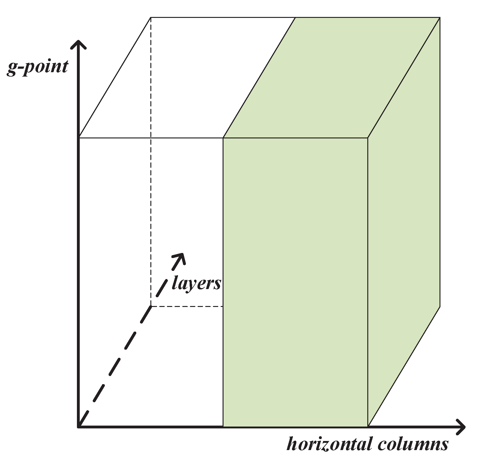
n l a y , the number of model layers in the vertical direction of the RRTMG_LW, is 51 in the CAS–ESM. Besides the parallelization in the horizontal direction, the one in the vertical direction for the RRTMG_LW is also considered to make full use of the performance of the GPU. Figure 4 illustrates the two-dimensional (2-D) domain decomposition for the RRTMG_LW accelerated on the GPU. The acceleration algorithm in the horizontal and vertical directions or with a 2-D domain decomposition for the RRTMG_LW is illustrated in Algorithm 4. Here, t B l o c k defines the number of threads used in each thread block of the x, y, and z dimensions by the derived type d i m 3 . g r i d defines the number of blocks in the x, y, and z dimensions by d i m 3 . Because of data dependency, cldprmc and r t r n m c are unsuitable for the parallelization in the vertical direction. These kernels with 2-D decomposition in Algorithm 4 are described as follows:
(1) The implementation of CUDA-based i n a t m _ d with 2-D decomposition is illustrated in Algorithm 5. Here, t h r e a d I d x % x identifies a unique thread inside a thread block in the x dimension, b l o c k I d x % x identifies a unique thread block inside a kernel grid in the x dimension, and b l o c k D i m % x identifies the number of threads in a thread block in the x dimension. In the same way, t h r e a d I d x % y , b l o c k I d x % y , and b l o c k D i m % y identify the corresponding configuration in the y dimension. l a y , the coordinate of the vertical direction, also represents the ID of a global thread in the y dimension, which can be expressed as l a y = ( b l o c k I d x % y 1 ) × b l o c k D i m % y + t h r e a d I d x % y . Therefore, a grid point in the horizontal and vertical directions can be identified by the i p l o n and l a y variables as two-dimensional linear data.
Due to data dependency, a piece of code in i n a t m _ d can be parallel only in the horizontal direction, so the kernel i n a t m _ d 3 in Algorithm 4 uses 1-D decomposition. The other code in i n a t m _ d is able to use 2-D decomposition. Due to the requirement of data synchronization, i n a t m _ d with the 2-D decomposition is divided into four kernels ( i n a t m _ d 1 , i n a t m _ d 2 , i n a t m _ d 3 , and i n a t m _ d 4 ). The 2-D parallelization of i n a t m _ d 1 , i n a t m _ d 2 , and i n a t m _ d 4 is similar to Algorithm 5. Their detailed implementations will not be described further here. According to the design shown in Algorithm 5, n c o l × n l a y e r s threads can execute 2-D i n a t m _ d concurrently.
(2) Similarly, due to data dependency, a piece of code in s e t c o e f _ d can be parallel only in the horizontal direction, so the kernel s e t c o e f _ d 2 in Algorithm 4 uses 1-D decomposition. The other code in s e t c o e f _ d is able to use 2-D decomposition, as shown in the kernel s e t c o e f _ d 1 . The 2-D parallelization of s e t c o e f _ d 1 is described in rough form in Algorithm A5 of Appendix A.2.
(3) The 2-D acceleration algorithm of t a u m o l _ d is illustrated in Algorithm A6 of Appendix A.2. Here, the 2-D parallelization of t a u g b 1 _ d with the device attribute is also described. The 2-D parallelization of the other 15 subroutines ( t a u g b 2 _ d t a u g b 16 _ d ) is similar to t a u g b 1 _ d .
Algorithm 4: CUDA-based acceleration algorithm of RRTMG_LW with 2-D domain decomposition and the implementation of 2-D G-RRTMG_LW.
subroutinerrtmg_lw_d2(parameters)
1.  Copy input data to GPU device
     //Call inatm_d1 with 2-D decomposition
2.  call inatm_d1 g r i d , t B l o c k (parameters)
     //Call inatm_d2 with 2-D decomposition
3.  call inatm_d2 g r i d , t B l o c k (parameters)
     //Call inatm_d3 with 1-D decomposition
4.  call inatm_d3 m , n (parameters)
     //Call inatm_d4 with 2-D decomposition
5.  call inatm_d4 g r i d , t B l o c k (parameters)
     //Call cldprmc_d with 1-D decomposition
6.  call cldprmc_d m , n (parameters)
     //Call setcoef_d1 with 2-D decomposition
7.  call setcoef_d1 g r i d , t B l o c k (parameters)
     //Call setcoef_d2 with 1-D decomposition
8.  call setcoef_d2 m , n (parameters)
     //Call taumol_d with 2-D decomposition
9.  call taumol_d g r i d , t B l o c k (parameters)
    //Call rtrnmc_d with 1-D decomposition
10.call rtrnmc_d m , n (parameters)
11.Copy result to host
     //Judge whether atmospheric horizontal profile data is completed
12.if it is not completed goto 1
end subroutine
Algorithm 5: Implementation of inatm_d based on CUDA Fortran in 2-D decomposition.
attributes(global) subroutine inatm_d(parameters)
1.  iplon = (blockIdx%x − 1) × blockDim%x + threadIdx%x
2.  lay = (blockIdx%y − 1) × blockDim%y + threadIdx%y
3.  if ((iplon≥1 .and. iplon≤ncol) .and. (lay≥1 .and. lay≤nlayers-1)) then
4.     Initialize variable arrays
5.     do ig = 1, ngptlw
6.        cldfmc(ig,iplon,lay) = cldfmcl_d(ig,iplon,nlayers-lay)
7.        taucmc(ig,iplon,lay) = taucmcl_d(ig,iplon,nlayers-lay)
8.        ciwpmc(ig,iplon,lay) = ciwpmcl_d(ig,iplon,nlayers-lay)
9.        clwpmc(ig,iplon,lay) = clwpmcl_d(ig,iplon,nlayers-lay)
10.   end do
11. end if
end subroutine

5. Result and Discussion

To fully investigate the parallel performance of the proposed acceleration algorithms described above, an ideal climate simulation experiment for one model day was conducted. The time step of the RRTMG_LW in the experiment was 1 h.

5.1. Performance of 1-D G-RRTMG_LW

5.1.1. Influence of Block Size

The run-time of the serial RRTMG_LW on one core of an Intel Xeon E5-2680 v2 processor is shown in Table 2. Here, the computing time of the RRTMG_LW on the CPU or GPU, T r r t m g _ l w , is calculated by the following formula:
T r r t m g _ l w = T i n a t m + T c l d p r m c + T s e t c o e f + T t a u m o l + T r t r n m c ,
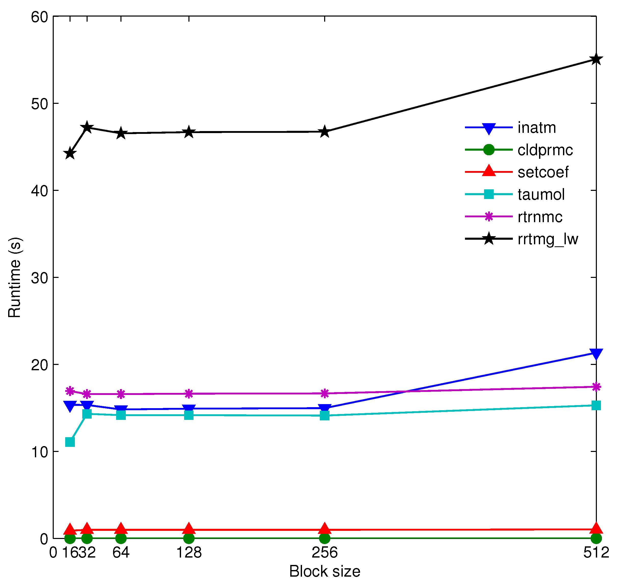
where T i n a t m is the computing time of the subroutine i n a t m or kernel i n a t m _ d and where T c l d p r m c , T s e t c o e f , T t a u m o l , and T r t r n m c are the corresponding computing time of the other kernels. To explore whether/how the number of threads in a thread block may affect the computation performance for a given scale, the execution time of the G-RRTMG_LW with a tuned number of threads was measured over one GPU. Taking the case of no I/O transfer as an example, Figure 5 portrays the run-time of the 1-D G-RRTMG_LW on one K20 GPU. Indeed, the number of threads per block or block size affected the computation performance to some extent. The G-RRTMG_LW achieved optimal performance when block size was 16. The G-RRTMG_LW on one K40 GPU resulted in a similar rule, as shown in Figure 6. Some conclusions and analysis are drawn as follows.
(1)
Generally speaking, increasing the block size can hide memory access latency to some extent and can improve the computational performance of parallel algorithms. Therefore, kernels with simple computations usually show optimal performance when the block size is 128 or 256.
(2)
The kernel t a u m o l with a large amount of calculation achieved optimal performance when the block size was 16. With the increment of the block size, its computational time increased as a whole. During the 1-D acceleration of t a u m o l , each thread with a large amount of calculation produced numerous temporary and intermediate values, which consumed a great deal of hardware resources. Due to limited hardware resources, each thread will have fewer resources if the block size is larger. Therefore, along with the increase of the block size, the speed of t a u m o l will be slower.

5.1.2. Evaluations on Different GPUs

The run-time and speedup of the 1-D G-RRTMG_LW on the K20 and K40 GPUs are shown in Table 2. The speedups of the 1-D i n a t m , c l d p r m c , s e t c o e f , t a u m o l , and r t r n m c on one K20 GPU were 7.36×, 2635.00×, 14.65×, 9.22×, and 11.83×, respectively. Using one K20 GPU in the case without I/O transfer, the 1-D G-RRTMG_LW achieved a speedup of 10.57× compared to its counterpart running on one CPU core of an Intel Xeon E5-2680 v2 whereas, using one K40 GPU in the case without I/O transfer, the 1-D G-RRTMG_LW achieved a speedup of 14.62×. The K40 GPU had higher core clock and memory clock, more cores, and stronger floating-point computation power than the K20 GPU, so the 1-D G-RRTMG_LW on the K40 GPU showed better performance.

5.2. Performance of 2-D G-RRTMG_LW

5.2.1. Influence of Block Size

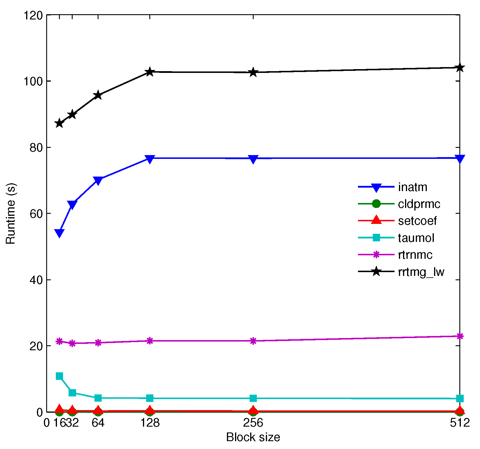
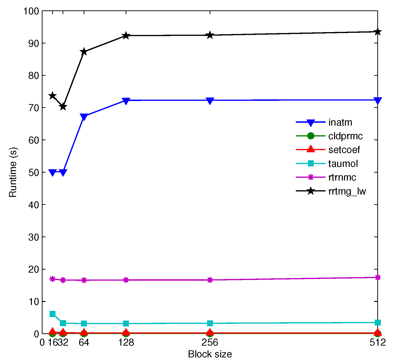
Taking the case of no I/O transfer as an example, Figure 7 portrays the run-time of the 2-D G-RRTMG_LW on one K20 GPU. The G-RRTMG_LW on one K20 GPU achieved optimal performance when the block size was 16. However, the 2-D G-RRTMG_LW on one K40 GPU achieved optimal performance when the block size was 32, as shown in Figure 8. The 2-D s e t c o e f and t a u m o l achieved a better speedup than their 1-D versions, but the 2-D i n a t m ran more slowly. From Figure 7 and Figure 8, some conclusions and analysis are drawn as follows.
(1)
The 2-D i n a t m costs more computational time than its 1-D version. This indicated that i n a t m was not fit for 2-D acceleration. According to the testing, it was found that the assignment computing of four three-dimensional arrays in the 2-D i n a t m required about 95% of the computational time. In the 2-D acceleration, more CUDA threads were started. Each CUDA thread needs to finish the assignment computing of the four arrays using a do-loop form as shown in Algorithm 5, so the computing costs too much time.
(2)
The 2-D t a u m o l achieved optimal performance when the block size was 256 or 512. During the 2-D acceleration, a larger number of threads were assigned, so each thread had fewer calculations, requiring fewer hardware resources. When the block size was 256 or 512, the assigned hardware resources of each thread were in a state of equilibrium, so in this case, the 2-D t a u m o l showed better performance.

5.2.2. Evaluations on Different GPUs

The run-time and speedup of the 2-D G-RRTMG_LW on the K20 and K40 GPUs are shown in Table 3. Due to the poor performance of the 2-D i n a t m , its 1-D version was still used here. The speedups of the 2-D s e t c o e f and t a u m o l on one K20 GPU were 43.21× and 40.54×, respectively. Using one K20 GPU in the case without I/O transfer, the 2-D G-RRTMG_LW achieved a speedup of 14.63× compared to its counterpart running on one CPU core of an Intel Xeon E5-2680 v2 whereas, using one K40 GPU in the case without I/O transfer, the 2-D G-RRTMG_LW achieved a speedup of 18.52×. Some conclusions and analysis are drawn as follows.
(1)
In the same way, the K40 GPU had stronger computing power than the K20 GPU, the 2-D G-RRTMG_LW on the K40 GPU showed better performance.
(2)
The 2-D s e t c o e f and t a u m o l showed excellent performance improvements compared to their 1-D versions, especially t a u m o l . There was no data dependence in t a u m o l with intensive computing, so a finer-grained parallelization of t a u m o l was executed when more threads were used.

5.3. I/O Transfer

I/O transfer between CPU and GPU is inevitable. The run-time and speedup of the 2-D G-RRTMG_LW with I/O transfer on the K20 and K40 GPUs are shown in Table 4. The I/O transfer times on the K20 cluster were 61.39 s and, on the K40 cluster, was 59.3 s. Using one K40 GPU in the case with I/O transfer, the 2-D G-RRTMG_LW achieved a speedup of 6.87×. Some conclusions and analysis are drawn as follows.
(1)
In the simulation with one model day, the RRTMG_LW required integral calculations 24 times. During each integration for all 128 × 256 grid points, the subroutine r r t m g _ l w must be invoked 16 (128 × 256/ n c o l ) times when n c o l is 2048. Due to the memory limitation of the GPU, the maximum value of n c o l on the K40 GPU was 2048. This means that the 2-D G-RRTMG_LW was invoked repeatedly 16 × 24 = 384 times in the experiment. For each invocation, the input and output of the three-dimensional arrays must be updated between the CPU and GPU, so the I/O transfer incurs a high communication cost.
(2)
After the 2-D acceleration for the RRTMG_LW, its computational time in the case without I/O transfer was fairly shorter, so the I/O transfer cost was a huge bottleneck for the maximum level of performance improvement of the G-RRTMG_LW. In the future, compressing data and improving network bandwidth will be beneficial for reducing this I/O transfer cost.

5.4. Discussion

(1)
The WRF RRTMG_LW on eight CPU cores achieved a speedup of 7.58× compared to its counterpart running on one CPU core [28]. Using one K40 GPU in the case without I/O transfer, the 2-D G-RRTMG_LW achieved a speedup of 18.52×. This shows that the RRTMG_LW on one GPU can still obtain a better performance improvement than on one CPU with eight cores.
(2)
The RRTM_LW on the C2050 obtained an 18.2× speedup [13]. This shows that the 2-D G-RRTMG_LW obtained a similar speedup with the RRTM_LW accelerated in CUDA Fortran.
(3)
The CUDA Fortran version of the RRTM_LW in the GRAPES_Meso model obtained a 14.3× speedup [27], but the CUDA C version of the RRTMG_SW obtained a 202× speedup [31]. The reasons are as follows. (a) Zheng et al. ran the original serial RRTM_LW on Intel Xeon 5500 and ran its GPU version on NVIDIA Tesla C1060. Mielikainen et al. ran the original serial RRTMG_SW on Intel Xeon E5-2603 and ran its GPU version on NVIDIA K40. Xeon 5500 has higher computing performance than Xeon E5-2603. Moreover, K40 has higher computing performance than Tesla C1060. Therefore, Mielikainen et al. obtained higher speedup. (b) Zheng et al. used CUDA Fortran to write the GPU code. Mielikainen et al. used CUDA C to write the GPU code. CUDA C with more mature techniques usually can perform better than CUDA Fortran.
(4)
If there is no I/O transfer between the CPU and GPU, the highest speedup value expected for theoretical algorithms of numerical schemes during GPU parallelization is equal to the number of CUDA threads started in the accelerating. One K40 GPU has 2880 CUDA cores, so the highest speedup value of the 2-D G-RRTMG_LW on one K40 GPU should be 2880. Due to the limitation of GPU memory and inevitable I/O transfer cost, it is very hard to get the theoretical speedup. However, the acceleration algorithm can be optimized further and I/O transfer cost between the CPU and GPU can be reduced to the furthest.

6. Conclusions and Future Work

High-efficiency parallel computing for radiation physics is exceedingly challenging. This paper presents the acceleration of the RRTMG_LW on GPU clusters. First, a GPU-based acceleration algorithm with a one-dimensional domain decomposition was proposed. Then, a second GPU-based acceleration algorithm with a two-dimensional domain decomposition was put forward. The two acceleration algorithms of the RRTMG_LW were implemented in CUDA Fortran. The G-RRTMG_LW, the GPU version of the RRTMG_LW, was also developed. The experimental results indicated that the 2-D G-RRTMG_LW displayed better calculation performances. During the computation of one model day, the 2-D G-RRTMG_LW on one K40 GPU obtained a speedup of 18.52× as compared to a single Intel Xeon E5-2680 CPU-core counterpart, with the run-time decreasing from 647.12 s to 34.9384 s. Due to the acceleration of the G-RRTMG_LW, the CAS–ESM achieved faster computing.
The current implementation of the G-RRTMG_LW did not achieve an acceptable speedup. The future work to address this includes the following two aspects. (1) The G-RRTMG_LW will be further accelerated. It may be beneficial to accelerate the G-RRTMG_LW in the g- p o i n t dimension. A GPU-based acceleration algorithm with a three-dimensional domain decomposition for the G-RRTMG_LW will be attempted to explore this idea. (2) The G-RRTMG_LW currently only runs on one GPU. However, on the K20 cluster, one node is equipped with 20 CPU cores and 2 GPU cards. To fully use the CPU cores and GPUs in this type of installation, an MPI+OpenMP+CUDA hybrid paradigm [38] will be considered. However, such a programming model will be a huge challenge in the implementation. Without a doubt, the G-RRTMG_LW on multiple GPUs will obtain even better computational performances.

Author Contributions

Conceptualization, Y.W.; methodology, Y.W., Y.Z., and J.J.; supervision, X.J. and A.Y.Z.; validation, Y.W. and Y.Z.; writing—original draft, Y.W.; writing—review and editing, Y.W. and W.L.

Funding

This work was supported in part by the National Key Research and Development Program of China under Grant 2016YFB0200800, in part by the National Natural Science Foundation of China under Grant 61602477, in part by the China Postdoctoral Science Foundation under Grant 2016M601158, in part by the Fundamental Research Funds for the Central Universities under Grant 2652017113, and in part by the Open Research Project of the Hubei Key Laboratory of Intelligent Geo-Information Processing under Grant KLIGIP-2017A04.

Acknowledgments

The authors would like to acknowledge the contributions of Minghua Zhang for insightful suggestions on the algorithm design.

Conflicts of Interest

The authors declare no conflict of interest.The funders had no role in the design of the study; in the collection, analyses, or interpretation of data; in the writing of the manuscript; or in the decision to publish the results.

Abbreviations

The following abbreviations are used in this manuscript:
HPChigh-performance computing
ESMearth system model
GPUgraphics processing unit
CPUcentral processing unit
CUDAcompute unified device architecture
GCMgeneral circulation model
LBLRTMline-by-line radiative transfer model
RRTMrapid radiative transfer model
RRTMGrapid radiative transfer model for general circulation models
CAS–ESMChinese Academy of Sciences–Earth System Model
IAPInstitute of Atmospheric Physics
IAP AGCM4.0IAP Atmospheric General Circulation Model Version 4.0
RRTMG_LWRRTMG long-wave radiation scheme
G-RRTMG_LWGPU version of the RRTMG_LW
WRFWeather Research and Forecasting model
RRTM_LWRRTM long-wave radiation scheme
RRTMG_SWRRTMG shortwave radiation scheme
HOMMEHigh-Order Methods Modeling Environment
AERAtmospheric and Environmental Research
RRTM_SWRRTM shortwave radiation scheme
McICAMonte–Carlo Independent Column Approximation
SMstreaming multiprocessor
SPstreaming processors
1-Done-dimensional
2-Dtwo-dimensional

Appendix A

Appendix A.1. Implementation of the Other Kernels Based on CUDA Fortran in 1-D Decomposition

Algorithm A1: Implementation of cldprmc_d based on CUDA Fortran in 1-D decomposition.
attributes(global) subroutine cldprmc_d(parameters)
1.  iplon = (blockIdx%x−1) × blockDim%x + threadIdx%x
2.  if (iplon≥1 .and. iplon≤ncol) then
3.     Initialize variable arrays
4.     do lay = 1, nlayers
5.        do ig = 1, ngptlw
6.           do some corresponding work
7.        end do
8.     end do
9.  end if
end subroutine
Algorithm A2: Implementation of setcoef_d based on CUDA Fortran in 1-D decomposition.
attributes(global) subroutine setcoef_d(parameters)
1.  iplon=(blockIdx%x−1) × blockDim%x+threadIdx%x
2.  if (iplon≥1 .and. iplon≤ncol) then
3.     Initialize variable arrays
        //Calculate the integrated Planck functions for each band at the surface, level, and layer
        //temperatures
4.     do lay = 1, nlayers
5.        do iband = 1, 16
6.          do some corresponding work
7.       end do
8.     end do
9. end if
end subroutine
Algorithm A3: Implementation of taumol_d based on CUDA Fortran in 1-D decomposition.
attributes(global) subroutine taumol_d(parameters)
1.  iplon=(blockIdx%x−1) × blockDim%x+threadIdx%x
2.  if (iplon≥1 .and. iplon≤ncol) then
        //Calculate gaseous optical depth and Planck fractions for each spectral band
3.     call taugb1_d(parameters)
4.     call taugb2_d(parameters)
5.     call taugb3_d(parameters)
6.     call taugb4_d(parameters)
7.     call taugb5_d(parameters)
8.     call taugb6_d(parameters)
9.     call taugb7_d(parameters)
10.   call taugb8_d(parameters)
11.   call taugb9_d(parameters)
12.   call taugb10_d(parameters)
13.   call taugb11_d(parameters)
14.   call taugb12_d(parameters)
15.   call taugb13_d(parameters)
16.   call taugb14_d(parameters)
17.   call taugb15_d(parameters)
18.   call taugb16_d(parameters)
19.end if
end subroutine
attributes(device) subroutine taugb1_d(parameters)
    //Lower atmosphere loop
    //laytrop is tropopause layer index
1. do lay = 1, laytrop(iplon)
       //ng1 is an integer parameter used for 140 g-point model
2.     do ig = 1, ng1
3.        do some corresponding work
4.     end do
5. end do
     //Upper atmosphere loop
6.  do lay = laytrop(iplon)+1, nlayers
7.     do ig = 1, ng1
8.        do some corresponding work
9.     end do
10.end do
end subroutine
Algorithm A4: Implementation of rtrnmc_d based on CUDA Fortran in 1-D decomposition.
attributes(global) subroutine rtrnmc_d(parameters)
1.  iplon=(blockIdx%x−1) × blockDim%x+threadIdx%x
2.  if (iplon≥1 .and. iplon≤ncol) then
3.     Initialize variable arrays
4.     do lay = 1, nlayers
5.        do ig = 1, ngptlw
6.          do some corresponding work
7.        end do
8.     end do
       //Loop over frequency bands
       //istart is beginning band of calculation
       //iend is ending band of calculation
9.     do iband = istart, iend
           //Downward radiative transfer loop
10.      do lay = nlayers, 1, −1
11.         do some corresponding work
12.      end do
13.   end do
14.end if
end subroutine

Appendix A.2. Implementation of the Other Kernels Based on CUDA Fortran in 2-D Decomposition

Algorithm A5: Implementation of setcoef_d based on CUDA Fortran in 2-D decomposition.
attributes(global) subroutine setcoef_d(parameters)
1.  iplon=(blockIdx%x−1) × blockDim%x+threadIdx%x
2.  lay=(blockIdx%y−1) × blockDim%y+threadIdx%y
3.  if ((iplon≥1 .and. iplon≤ncol) .and. (lay≥1 .and. lay≤nlayers)) then
4.     Initialize variable arrays
5.     do iband = 1, 16
6.       do some corresponding work
7.     end do
8.  end if
end subroutine
Algorithm A6: Implementation of taumol_d based on CUDA Fortran in 2-D decomposition.
attributes(global) subroutine taumol_d(parameters)
1.  iplon=(blockIdx%x−1) × blockDim%x+threadIdx%x
2.  lay=(blockIdx%y−1) × blockDim%y+threadIdx%y
3.  if ((iplon≥1 .and. iplon≤ncol) .and. (lay≥1 .and. lay≤nlayers)) then
4.     call taugb1_d(parameters)
5.     call taugb2_d(parameters)
6.     call taugb3_d(parameters)
7.     call taugb4_d(parameters)
8.     call taugb5_d(parameters)
9.     call taugb6_d(parameters)
10.   call taugb7_d(parameters)
11.   call taugb8_d(parameters)
12.   call taugb9_d(parameters)
13.   call taugb10_d(parameters)
14.   call taugb11_d(parameters)
15.   call taugb12_d(parameters)
16.   call taugb13_d(parameters)
17.   call taugb14_d(parameters)
18.   call taugb15_d(parameters)
19.   call taugb16_d(parameters)
20.end if
end subroutine
attributes(device) subroutine taugb1_d(parameters)
1.  if ((iplon≥1 .and. iplon≤ncol) .and. (lay≥1 .and. lay≤laytrop(iplon))) then
2.     do ig = 1, ng1
3.        do some corresponding work
4.     end do
5.  end if
6.  if ((iplon≥1 .and. iplon≤ncol) .and. (lay≥laytrop(iplon)+1 .and. lay≤nlayers)) then
7.     do ig = 1, ng1
8.        do some corresponding work
9.     end do
10.end if
end subroutine

References

  1. Xue, W.; Yang, C.; Fu, H.; Wang, X.; Xu, Y.; Liao, J.; Gan, L.; Lu, Y.; Ranjan, R.; Wang, L. Ultra-scalable CPU-MIC acceleration of mesoscale atmospheric modeling on tianhe-2. IEEE Trans. Comput. 2014, 64, 2382–2393. [Google Scholar] [CrossRef]
  2. Imbernon, B.; Prades, J.; Gimenez, D.; Cecilia, J.M.; Silla, F. Enhancing large-scale docking simulation on heterogeneous systems: An MPI vs. rCUDA study. Future Gener. Comput. Syst. 2018, 79, 26–37. [Google Scholar] [CrossRef]
  3. Lu, G.; Zhang, W.; He, H.; Yang, L.T. Performance modeling for MPI applications with low overhead fine-grained profiling. Future Gener. Comput. Syst. 2019, 90, 317–326. [Google Scholar] [CrossRef]
  4. Wang, Y.; Jiang, J.; Zhang, J.; He, J.; Zhang, H.; Chi, X.; Yue, T. An efficient parallel algorithm for the coupling of global climate models and regional climate models on a large-scale multi-core cluster. J. Supercomput. 2018, 74, 3999–4018. [Google Scholar] [CrossRef]
  5. Nickolls, J.; Dally, W.J. The GPU computing era. IEEE Micro 2010, 30, 56–69. [Google Scholar] [CrossRef]
  6. Deng, Z.; Chen, D.; Hu, Y.; Wu, X.; Peng, W.; Li, X. Massively parallel non-stationary EEG data processing on GPGPU platforms with Morlet continuous wavelet transform. J. Internet Serv. Appl. 2012, 3, 347–357. [Google Scholar] [CrossRef] [Green Version]
  7. Chen, D.; Wang, L.; Tian, M.; Tian, J.; Wang, S.; Bian, C.; Li, X. Massively parallel modelling & simulation of large crowd with GPGPU. J. Supercomput. 2013, 63, 675–690. [Google Scholar]
  8. Chen, D.; Li, X.; Wang, L.; Khan, S.U.; Wang, J.; Zeng, K.; Cai, C. Fast and scalable multi-way analysis of massive neural data. IEEE Trans. Comput. 2015, 64, 707–719. [Google Scholar] [CrossRef]
  9. Candel, F.; Petit, S.; Sahuquillo, J.; Duato, J. Accurately modeling the on-chip and off-chip GPU memory subsystem. Future Gener. Comput. Syst. 2018, 82, 510–519. [Google Scholar] [CrossRef]
  10. Norman, M.; Larkin, J.; Vose, A.; Evans, K. A case study of CUDA FORTRAN and OpenACC for an atmospheric climate kernel. J. Comput. Sci. 2015, 9, 1–6. [Google Scholar] [CrossRef] [Green Version]
  11. Schalkwijk, J.; Jonker, H.J.; Siebesma, A.P.; Van Meijgaard, E. Weather forecasting using GPU-based large-eddy simulations. Bull. Am. Meteorol. Soc. 2015, 96, 715–723. [Google Scholar] [CrossRef]
  12. NVIDIA. CUDA C Programming Guide v10.0. Technical Document. 2019. Available online: Https://docs.nvidia.com/pdf/CUDA_C_Programming_Guide.pdf (accessed on 26 September 2019).
  13. Lu, F.; Cao, X.; Song, J.; Zhu, X. GPU computing for long-wave radiation physics: A RRTM_LW scheme case study. In Proceedings of the IEEE 9th International Symposium on Parallel and Distributed Processing with Applications Workshops (ISPAW), Busan, Korea, 26–28 May 2011; pp. 71–76. [Google Scholar]
  14. Clough, S.A.; Iacono, M.J.; Moncet, J.L. Line-by-line calculations of atmospheric fluxes and cooling rates: Application to water vapor. J. Geophys. Res. Atmos. 1992, 97, 15761–15785. [Google Scholar] [CrossRef]
  15. Clough, S.A.; Iacono, M.J. Line-by-line calculation of atmospheric fluxes and cooling rates II: Application to carbon dioxide, ozone, methane, nitrous oxide and the halocarbons. J. Geophys. Res. Atmos. 1995, 100, 16519–16535. [Google Scholar] [CrossRef]
  16. Lu, F.; Song, J.; Cao, X.; Zhu, X. CPU/GPU computing for long-wave radiation physics on large GPU clusters. Comput. Geosci. 2012, 41, 47–55. [Google Scholar] [CrossRef]
  17. Mlawer, E.J.; Taubman, S.J.; Brown, P.D.; Iacono, M.J.; Clough, S.A. Radiative transfer for inhomogeneous atmospheres: RRTM, a validated correlated-k model for the long-wave. J. Geophys. Res. Atmos. 1997, 102, 16663–16682. [Google Scholar] [CrossRef]
  18. Clough, S.A.; Shephard, M.W.; Mlawer, E.J.; Delamere, J.S.; Iacono, M.J.; Cady-Pereira, K.; Boukabara, S.; Brown, P.D. Atmospheric radiative transfer modeling: A summary of the AER codes. J. Quant. Spectrosc. Radiat. Transf. 2005, 91, 233–244. [Google Scholar] [CrossRef]
  19. Iacono, M.J.; Mlawer, E.J.; Clough, S.A.; Morcrette, J.J. Impact of an improved long-wave radiation model, RRTM, on the energy budget and thermodynamic properties of the NCAR community climate model, CCM3. J. Geophys. Res. Atmos. 2000, 105, 14873–14890. [Google Scholar] [CrossRef]
  20. Iacono, M.J.; Delamere, J.S.; Mlawer, E.J.; Shephard, M.W.; Clough, S.A.; Collins, W.D. Radiative forcing by long-lived greenhouse gases: Calculations with the AER radiative transfer models. J. Geophys. Res. Atmos. 2008, 113. [Google Scholar] [CrossRef]
  21. Xiao, D.; Tong-Hua, S.; Jun, W.; Ren-Ping, L. Decadal variation of the Aleutian Low-Icelandic Low seesaw simulated by a climate system model (CAS–ESM-C). Atmos. Ocean. Sci. Lett. 2014, 7, 110–114. [Google Scholar] [CrossRef]
  22. Wang, Y.; Jiang, J.; Ye, H.; He, J. A distributed load balancing algorithm for climate big data processing over a multi-core CPU cluster. Concurr. Comput. Pract. Exp. 2016, 28, 4144–4160. [Google Scholar] [CrossRef]
  23. Wang, Y.; Hao, H.; Zhang, J.; Jiang, J.; He, J.; Ma, Y. Performance optimization and evaluation for parallel processing of big data in earth system models. Clust. Comput. 2017. [Google Scholar] [CrossRef]
  24. Zhang, H.; Zhang, M.; Zeng, Q.C. Sensitivity of simulated climate to two atmospheric models: Interpretation of differences between dry models and moist models. Mon. Weather. Rev. 2013, 141, 1558–1576. [Google Scholar] [CrossRef]
  25. Wang, Y.; Jiang, J.; Zhang, H.; Dong, X.; Wang, L.; Ranjan, R.; Zomaya, A.Y. A scalable parallel algorithm for atmospheric general circulation models on a multi-core cluster. Future Gener. Comput. Syst. 2017, 72, 1–10. [Google Scholar] [CrossRef] [Green Version]
  26. Morcrette, J.J.; Mozdzynski, G.; Leutbecher, M. A reduced radiation grid for the ECMWF Integrated Forecasting System. Mon. Weather Rev. 2008, 136, 4760–4772. [Google Scholar] [CrossRef]
  27. Zheng, F.; Xu, X.; Xiang, D.; Wang, Z.; Xu, M.; He, S. GPU-based parallel researches on RRTM module of GRAPES numerical prediction system. J. Comput. 2013, 8, 550–558. [Google Scholar] [CrossRef]
  28. Iacono, M.J. Enhancing Cloud Radiative Processes and Radiation Efficiency in the Advanced Research Weather Research and Forecasting (WRF) Model; Atmospheric and Environmental Research: Lexington, MA, USA, 2015. [Google Scholar]
  29. NVIDIA. CUDA Fortran Programming Guide and Reference. Technical Document. 2019. Available online: Https://www.pgroup.com/resources/docs/19.1/pdf/pgi19cudaforug.pdf (accessed on 26 September 2019).
  30. Ruetsch, G.; Phillips, E.; Fatica, M. GPU acceleration of the long-wave rapid radiative transfer model in WRF using CUDA Fortran. In Proceedings of the Many-Core and Reconfigurable Supercomputing Conference, Roma, Italy, 22–24 March 2010. [Google Scholar]
  31. Mielikainen, J.; Price, E.; Huang, B.; Huang, H.L.; Lee, T. GPU compute unified device architecture (CUDA)-based parallelization of the RRTMG shortwave rapid radiative transfer model. IEEE J. Sel. Top. Appl. Earth Obs. Remote. Sens. 2016, 9, 921–931. [Google Scholar] [CrossRef]
  32. Bertagna, L.; Deakin, M.; Guba, O.; Sunderl, D.; Bradley, A.M.; Tezaur, I.K.; Taylor, M.A.; Salinger, A.G. HOMMEXX 1.0: A performance portable atmospheric dynamical core for the energy exascale earth system model. Geosci. Model Dev. 2018, 12, 1423–1441. [Google Scholar] [CrossRef]
  33. Iacono, M.J.; Delamere, J.S.; Mlawer, E.J.; Clough, S.A. Evaluation of upper tropospheric water vapor in the NCAR Community Climate Model (CCM3) using modeled and observed HIRS radiances. J. Geophys. Res. Atmos. 2003, 108, ACL 1-1–ACL 1-19. [Google Scholar] [CrossRef]
  34. Morcrette, J.J.; Barker, H.W.; Cole, J.N.; Iacono, M.J.; Pincus, R. Impact of a new radiation package, McRad, in the ECMWF Integrated Forecasting System. Mon. Weather Rev. 2008, 136, 4773–4798. [Google Scholar] [CrossRef]
  35. Mlawer, E.J.; Iacono, M.J.; Pincus, R.; Barker, H.W.; Oreopoulos, L.; Mitchell, D.L. Contributions of the ARM program to radiative transfer modeling for climate and weather applications. Meteorol. Monogr. 2016, 57, 15.1–15.19. [Google Scholar] [CrossRef]
  36. Pincus, R.; Barker, H.W.; Morcrette, J.J. A fast, flexible, approximate technique for computing radiative transfer in inhomogeneous cloud fields. J. Geophys. Res. Atmos. 2003, 108. [Google Scholar] [CrossRef]
  37. Price, E.; Mielikainen, J.; Huang, M.; Huang, B.; Huang, H.L.; Lee, T. GPU-accelerated long-wave radiation scheme of the Rapid Radiative Transfer Model for General Circulation Models (RRTMG). IEEE J. Sel. Top. Appl. Earth Obs. Remote Sens. 2014, 7, 3660–3667. [Google Scholar] [CrossRef]
  38. D’Azevedo, E.F.; Lang, J.; Worley, P.H.; Ethier, S.A.; Ku, S.H.; Chang, C. Hybrid MPI/OpenMP/GPU parallelization of xgc1 fusion simulation code. In Proceedings of the Supercomputing Conference 2013, Denver, CO, USA, 17–22 November 2013. [Google Scholar]
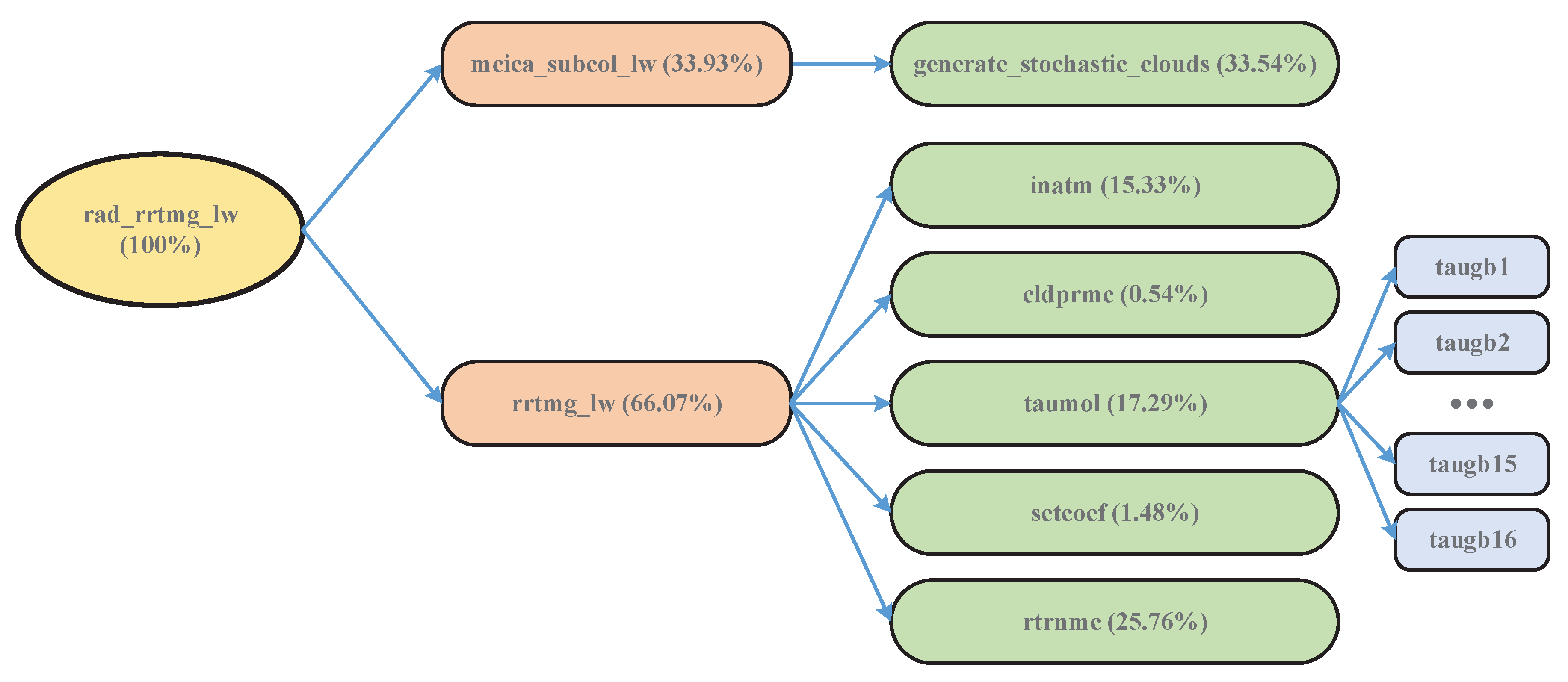
Figure 1. Profiling graph of the original rapid radiative transfer model for general circulation models (RRTMG) long-wave radiation scheme (RRTMG_LW) code in the Chinese Academy of Sciences–Earth System Model (CAS–ESM): Here, each arrow represents the invoking relation among subroutines.
Applsci 09 04039 g001
Figure 2. Three-dimensional spatial structure of RRTMG_LW: Its physical dimensions include longitude, latitude, and model layers.
Applsci 09 04039 g002
Figure 3. Schematic diagram of 1-D decomposition for the RRTMG_LW in the GPU acceleration.
Applsci 09 04039 g003
Figure 4. Schematic diagram of 2-D decomposition for the RRTMG_LW in the GPU acceleration.
Applsci 09 04039 g004
Figure 5. Run-time of the 1-D G-RRTMG_LW on one K20 GPU.
Applsci 09 04039 g005
Figure 6. Run-time of the 1-D G-RRTMG_LW on one K40 GPU.
Applsci 09 04039 g006
Figure 7. Run-time of the 2-D G-RRTMG_LW on one K20 GPU.
Applsci 09 04039 g007
Figure 8. Run-time of the 2-D G-RRTMG_LW on one K40 GPU.
Applsci 09 04039 g008
Table 1. Configurations of graphics processing unit (GPU) clusters.
Specification of Central Processing Unit (CPU)K20 ClusterK40 Cluster
CPUE5-2680 v2 at 2.8 GHzE5-2695 v2 at 2.4 GHz
Operating SystemCentOS 6.4Red Hat Enterprise Linux Server 7.1
Specification of GPUK20 clusterK40 cluster
GPUTesla K20Tesla K40
Compute Unified Device Architecture (CUDA) Cores24962880
Standard Memory5 GB12 GB
Memory Bandwidth208 GB/s288 GB/s
CUDA Version6.59.0
Table 2. Run-time and speedup of the 1-D G-RRTMG_LW on one GPU, where the block size = 16 and ncol = 2048.
SubroutinesCPU Time (s)K20 Time (s)Speedup
inatm150.4820.44407.36
cldprmc5.270.00202635.00
setcoef14.520.990814.65
taumol169.6818.39809.22
rtrnmc252.8021.371211.83
rrtmg_lw647.1261.20610.57
SubroutinesCPU Time (s)K40 Time (s)Speedup
inatm150.4815.34929.80
cldprmc5.270.00163293.75
setcoef14.520.892016.28
taumol169.6811.072015.33
rtrnmc252.8016.934414.93
rrtmg_lw647.1244.249214.62
Table 3. Run-time and speedup of the 2-D G-RRTMG_LW on one GPU, where the block size = 128 and ncol = 2048.
SubroutinesCPU Time (s)K20 Time (s)Speedup
inatm150.4818.20608.27
cldprmc5.270.00202635.00
setcoef14.520.336043.21
taumol169.684.185240.54
rtrnmc252.8021.514811.75
rrtmg_lw647.1244.244014.63
SubroutinesCPU Time (s)K40 Time (s)Speedup
inatm150.4814.906810.09
cldprmc5.270.00202635
setcoef14.520.248058.55
taumol169.683.152453.83
rtrnmc252.8016.629215.20
rrtmg_lw647.1234.938418.52
Table 4. Run-time and speedup of the 2-D G-RRTMG_LW with I/O transfer on one GPU, where the block size = 128 and ncol = 2048.
SubroutinesCPU Time (s)K20 Time (s)Speedup
rrtmg_lw647.12105.636.13
SubroutinesCPU Time (s)K40 Time (s)Speedup
rrtmg_lw647.1294.246.87