Automatic Object-Detection of School Building Elements in Visual Data: A Gray-Level Histogram Statistical Feature-Based Method

Abstract

Automatic object-detection technique can improve the efficiency of building data collection for semi-empirical methods to assess the seismic vulnerability of buildings at a regional scale. However, current structural element detection methods rely on color, texture and/or shape information of the object to be detected and are less flexible and reliable to detect columns or walls with unknown surface materials or deformed shapes in images. To overcome these limitations, this paper presents an innovative gray-level histogram (GLH) statistical feature-based object-detection method for automatically identifying structural elements, including columns and walls, in an image. This method starts with converting an RGB image (i.e. the image colors being a mix of red, green and blue light) into a grayscale image, followed by detecting vertical boundary lines using the Prewitt operator and the Hough transform. The detected lines divide the image into several sub-regions. Then, three GLH statistical parameters (variance, skewness, and kurtosis) of each sub-region are calculated. Finally, a column or a wall in a sub-region is recognized if these features of the sub-region satisfy the predefined criteria. This method was validated by testing the detection precision and recall for column and wall images. The results indicated the high accuracy of the proposed method in detecting structural elements with various surface treatments or deflected shapes. The proposed structural element detection method can be extended to detecting more structural characteristics and retrieving structural deficiencies from digital images in the future, promoting the automation in building data collection.

1. Introduction

Regional seismic vulnerability assessment of school buildings can provide civil-protection agencies with information crucial to optimal emergency planning and mitigation, including projections of the scale and distribution of building damages. Semi-empirical methods, which evaluate the seismic vulnerability of buildings based on a small range of building attributes selected by experts coupled with data-mining techniques, have proved its efficiency in rapidly assessing the seismic vulnerabilities of buildings at a large scale [1,2]. These building attributes include the number and sizes of structural elements (e.g., columns and walls), building heights, structural deficiencies (e.g., short columns and soft-stories), and so forth. However, existing data on building attributes at a regional scale are often incomplete or dispersed (e.g., available only as paper records spanning a number of bureaucratic departments), imposing limits on the effectiveness of vulnerability assessment [3]. Collecting such data anew, meanwhile, is costly, time-consuming, and expert-dependent because the traditional visual-screening approach to do so involves paper-based field surveys carried out by structural experts or certified engineers [4]. Moreover, human errors like mistaking the number of structural elements during field survey are commonplace, and such errors can reduce the reliability and accuracy of assessment results.

To overcome the limitations of field survey, computer vision technologies have been applied to data collection on building characteristics [5,6,7,8,9,10]. As columns and walls are basic load-bearing elements relevant to buildings’ seismic vulnerability, automatic recognition of columns and walls could provide important information for seismic vulnerability assessment of buildings. Previous research on the automated detection of columns commonly uses color/texture and shape features to recognize concrete columns because such columns are considered to be rectangular in shape with familiar color and texture on surfaces [11,12,13]. However, the color/texture-based detection techniques are unable to cope with the structural elements covered in unknown types of paint, tiling, or other surface treatments, which is common for school building columns, and the shape-based detection methods fail to work if structural elements deflect in images resulting from camera tilting or perspective illusion. Meanwhile, automated detection of walls using computer version technologies is still a lack of study.

This article reports on an innovative study that utilizes the gray-level histogram (GLH) statistical features and shape features, without relying on detecting familiar colors and surface materials or fixed shapes, to overcome the drawbacks of present automatic detection methods for columns and walls. Moreover, in the view of the practical application of the proposed method, every single person who can take images by their smartphones, cameras, or other devices should be able to collect information of columns and walls, with the images processed on personal computers, local devices, or cloud computing. With this in mind, the proposed method is based on a single image, without any technical requirements for image acquisition. Although this paper focuses on detecting and counting columns and walls in images, the proposed automatic detection method can be further extended to the detection of a wide range of structural elements’ characteristics (e.g., sizes and surface defects) and structural deficiencies (e.g., short columns and soft stories), promoting the automation in building data collection.

2. Background

Ideally, a holistic urban seismic risk assessment would investigate the behavior of every single building during seismic events via computational modeling. However, it is impractical to apply them at a regional scale because the computational models require detailed information of each building and it takes massive time to build models and execute structural analysis for hundreds of thousands of buildings. For vulnerability assessment to achieve adequate accuracy while avoiding exhaustive data collection and computational analysis, semi-empirical approaches have been developed: a few structural characteristics of buildings (e.g., the number and sizes of columns and walls, building height, and structural deficiencies) assessed by expert judgment are coupled with data-mining techniques to predict buildings’ seismic vulnerabilities [1,14,15]. Therefore, collecting structural information is the first step to successfully apply the semi-empirical approaches for building seismic vulnerability assessment at a regional scale. Realizing deficiencies of traditional paper-based field surveys, vision-based technologies have been applied to structural information collection.

A handful of prior studies on structural element detection methods can be generally classified into color/texture-based methods and shape-based methods: the former detects a structural element by judging if the color or texture of the object’s material matches the predefined material databases, and the latter by judging if the shape of the object matches the predefined element shape templates. However, structural elements in images may fail to match these predefined databases or templates because of their diversities in colors, textures, and shapes. Therefore, grayscale statistical feature-based object-detection methods, being able to detect objects without predefining databases or templates, are introduced in this section.

2.1. Color/Texture-Based Object Detection Methods

The color and texture of materials are commonly used in detecting structural elements since those elements are usually composed of a single material (e.g., concrete) [11,12,13,16]. Based on the finding that most color values of construction materials were in certain ranges, Abeid Neto et al. [17] identified a structural element by detecting its boundary pixels whose color values satisfied the predefined color ranges. Instead of taking into account color features only, Brilakis and Soibelman [18] combined both color and texture features to label regions in an image. A region was considered as a structural element, if the Euclidean distance between the region label and a predefined material label was smaller than a predefined threshold. Recently, machine learning techniques are widely used in detecting concrete structural elements by recognizing their materials [11,19,20,21,22]. The input data are those quantified color or texture characteristics, such as RGB values (the color depth of red, green, and blue light, ranging from 0 to 255) [23], luminance values [24], and filter bank responses [25].

However, color/texture-based methods are unable to cope with structural elements covered in unknown paint, tiles, or other surface treatments, which are common to be seen in school building columns and walls. Moreover, color/texture-based methods require a predefined material library, which is not only time-consuming to be built but also is unable to cover all characteristics of materials because even the same material can have different characteristics under different scenarios. For example, the color of a material can be different under various illumination intensities. Missing containing characteristics of materials can lead to the failure of detection.

2.2. Shape-Based Object Detection Methods

In addition to color and texture features, the edge information, indicating the boundary of an object and appearing in the area where image pixel intensity changes sharply, is another feature used for detecting structural elements. Shape-based object detection methods identify structural elements in images by detecting their edge lines. Jung and Schramm [26] detected rectangle objects which represent structural elements in images by searching their two pairs of parallel edge lines. Although this method performs well in detecting rectangle structural elements of different sizes and length-width ratios, the sole reliance on shape information narrows their applications in detecting slant or vague elements in images [27]. To improve such drawbacks, coupling shape information with color and texture features, Zhu and Brilakis [28] proposed a concrete column-detection method based on the assumptions that the shape of a single concrete column is bounded by a pair of long vertical lines, and the color and texture patterns on the surface of a concrete column are uniform and could be matched to a predefined color-pattern database for particular materials. Zhang et al. [29] used long edge lines as well as color features to locate a wall between two windows. Hamledari et al. [30] utilized both shape and color features to detect vertical indoor components of structures from 2D digital images during construction phases. Although such a combination improves the drawbacks of shape-based methods, it introduces the disadvantage of color/texture-based methods as aforementioned. In addition, current shape-based methods fail to work when vertical edge lines of structural elements deviate from the vertical direction because of camera tilting or perspective illusion.

2.3. Grayscale Statistical Feature-Based Object Detection Methods

Grayscale statistical feature-based methods utilize a set of statistical parameters extracted from grayscale pixel intensity of images to recognize objects. Generally, grayscale statistical parameters are classified into two groups: gray-level co-occurrence matrix (GLCM) statistical parameters and gray-level histogram (GLH) statistical parameters.

Haralick and Shanmugam [31] first introduced the GLCM, which described the frequency of one gray level appearing in a specified spatial linear relationship with another gray level within the area under investigation and originally proposed 14 GLCM statistical parameters to label the GLCM. From then on, these GLCM statistical parameters have been widely used in image recognition, such as detecting sea ice changing in images [32,33,34], classifying landscape images [35], and distinguishing computed tomography (CT) images of normal and abnormal tissues [36,37]. However, it is difficult to understand the essential meanings of GLCM statistical parameters and to visibly check how these GLCM parameters can affect detection results since GLCM statistical parameters represent abstract characteristics of an object. Accordingly, GLH statistical parameters (mean, variance, integrated intensity, skewness, and kurtosis), representing the distribution of the pixel intensity of an image, have been developed and used in image recognition [38,39,40]. Zhang and Wang [41] used GLH and GLCM statistical parameters respectively to classify normal and abnormal human brain CT images, and the results showed that the classification accuracy with GLH statistical parameters was higher than that with GLCM statistical parameters, proving GLH’s superiority in image classification. This result was also supported by Fallahi et al. [42]. In addition to medical use, An et al. [43] classified traffic signs with GLH statistical parameters and got a high classification accuracy rate.

The proposed method innovatively combines the GLH statistical parameters and shape features of structural elements to recognize columns and walls in images given that columns and walls have two distinguishing visual characteristics: (1) the gray levels of their surfaces are relatively homogeneous compared with their neighboring areas that contain various objects, and (2) their boundary edges are long vertical lines. Additionally, as some of GLH statistical parameters contribute little in representing specific objects, it is unnecessary to use all GLH parameters to detect objects. Thus, this study will select proper GLH parameters by considering both statistical meanings and visual meanings of these GLH parameters to decrease the computational cost for the detection of structural elements.

3. Methodology

As shown in Figure 1, this method starts with transforming an RGB image (i.e. the image colors are a mix of red, green and blue light) into a grayscale image. Then the Prewitt operator, coupled with the Hough transform, is used to detect long vertical lines in the grayscale image. Quadrilateral sub-regions could then be identified between two adjacent detected lines. Next, three GLH statistical parameters (variance, skewness, and kurtosis) of each sub-region are calculated. A structural element is recognized if the shape and the GLH statistical parameters of a sub-region satisfy our predefined criteria. Finally, the type of the element (a column or a wall) is determined according to the ratio of the sub-region’s length to width.

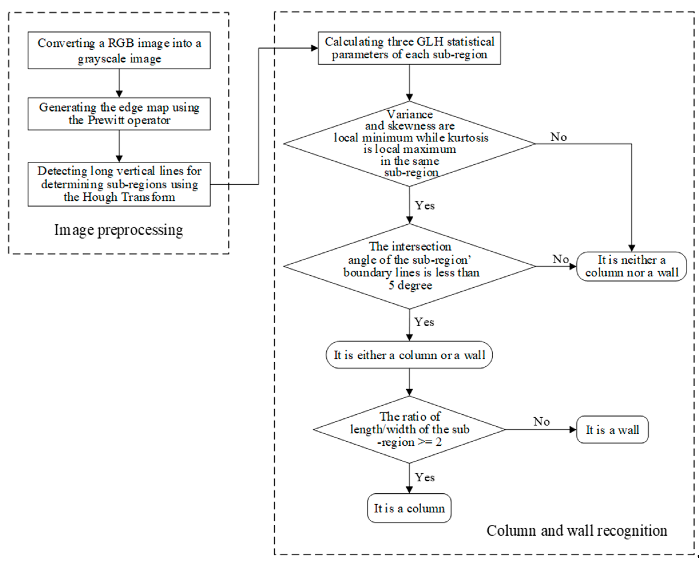
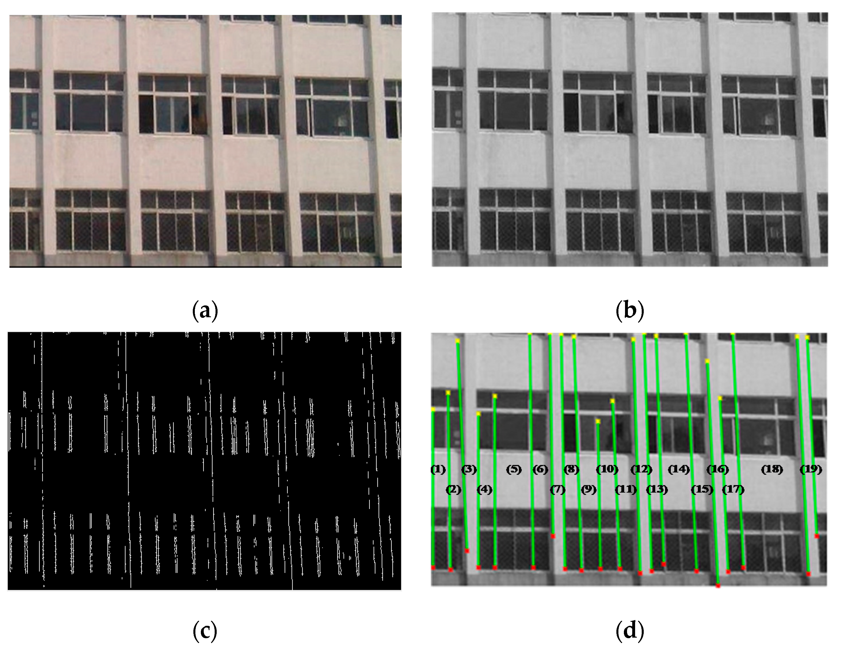
3.1. Image Preprocessing

In order to extract the GLH statistical parameters in later steps, the RGB image is firstly converted into a grayscale image using Equation (1),

$$f\left(x,y\right)=a_1\ast R\left(x,y\right)+a_2\ast G\left(x,y\right)+a_3\ast B\left(x,y\right),\forall a_1+a_2+a_3=1,$$

(1)

where $\left(x,y\right)$ is the location of a pixel in the pixel matrix of an image; $f\left(x,y\right)$ is the grayscale value comprising a pixel intensity level between 0 and 255; $R\left(x,y\right), G\left(x,y\right), B\left(x,y\right)$ represent the red, green and blue values of the pixel located in $\left(x,y\right)$, respectively; $a_1,a_2$ and $a_3$ are weighting factors that are automatically adjusted according to the R, G, B values of a given image.

An edge is defined as the abrupt change of gray levels in a grayscale image [44], providing indications of the physical extent of an object. In a continuous domain edge segment $F\left(x,y\right)$, the continuous gradient $G\left(x,y\right)$ is calculated along a certain direction. The edge is detected if the gradient$G\left(x,y\right)$ is above a given threshold value. The gradient $G\left(x,y\right)$ can be computed by Equation (2),

$$G\left(x,y\right)=\frac{\partial F\left(x,y\right)}{\partial x}cos\phi +\frac{\partial F\left(x,y\right)}{\partial y}sin\phi ,$$

(2)

where $\phi$ is the angle between $F\left(x,y\right)$ and the horizontal axis.

In a discrete grayscale image which is a $M\times N$ pixel matrix with $M$ rows and $N$ columns of pixels, a row gradient $G_R\left(j,k\right)$ and a column gradient $G_C\left(j,k\right)$ can be calculated using Equation (3),

$$\{\begin{array}{c}{G}_R\left(j,k\right)=F\left(j,k\right)-F\left(j,k-1\right), j=0,1,\dots ,M-1;k=0,1,\dots ,N-1;\\ G_C\left(j,k\right)=F\left(j,k\right)-F\left(j+1,k\right), j=0,1,\dots ,M-1;k=0,1,\dots ,N-1;\end{array},$$

(3)

where $\left(j,k\right)$ is the coordinate of a pixel in the matrix, in which the coordinate of the first pixel (in the top-left corner) is (0,0). The row and column gradients $G_R\left(j,k\right)$ and $G_C\left(j,k\right)$ can be alternatively computed by using impulse response matrix, Equation (4):

$$\{\begin{array}{c}{G}_R\left(j,k\right)=F\left(j,k\right)\times H_R\left(j,k\right)\\ G_C\left(j,k\right)=F\left(j,k\right)\times H_C\left(j,k\right)\end{array},$$

(4)

where $H_R\left(j,k\right)$ and $H_C\left(j,k\right)$ are row- and column-impulse response matrix, respectively, which can be defined by given edge-detection operators: the Prewitt operator [45], the Sobel operator [46], the Roberts operator [47], and the Canny operator [48]. Among these operators, the Prewitt operator is distinguished by its capability of detecting the horizontal and vertical edges [49], defined by Equation (5) and Equation (6), respectively:

$$H_R\left(j,k\right)=\frac{1}{3}\left[\begin{array}{ccc}1& 0& -1\\ 1& 0& -1\\ 1& 0& -1\end{array}\right]$$

(5)

$$H_C\left(j,k\right)=\frac{1}{3}\left[\begin{array}{ccc}-1& -1& -1\\ 0& 0& 0\\ 1& 1& 1\end{array}\right].$$

(6)

However, the edge-detection operator can only result in a discrete edge map composed of isolated boundary points without knowing which points lie on the same lines. Therefore, coupled with edge-detection operators, line-detection techniques should be used to extract lines from the discrete edge map.

The Hough transform [50] is widely used for retrieving line information from edge maps, due to its powerful ability in dealing with pixels that are missing or spurious as a result of noise produced by image defects or edge-detector imperfections. In a discrete binary image, such as an edge map produced by the Prewitt operator, each non-zero point $\left(x,y\right)$ in the Cartesian coordinate space is transformed into a line in the polar coordinate space$\left(\rho ,\theta \right)$ using Equation (7), where $\rho$ is the perpendicular distance from the image’s origin point to the line, restricted to [−D, D], with D being the half-diagonal size of the image; and $\theta$ is the angle between the normal of the line and the x-axis of the image, restricted to $\left[-90°,90°\right]$. After transformation, lines are quantized into cells $\mathrm{A}\left(\rho ,\theta \right)$ whose initial values are 0. Straight lines that are transformed from points lying on the same line in Cartesian coordinate space will intersect at the same point in polar coordinate space. Then, the number of straight lines intersecting at the point (${\rho }_i,{\theta }_i$) will be recorded in $\mathrm{A}\left({\rho }_i,{\theta }_i\right)$, which represents the number of edge points lying on the same straight line. After all detected edge points are processed, the $\mathrm{A}\left(\rho ,\theta \right)$ cells are examined. Large counts in cells $\mathrm{A}\left(\rho ,\theta \right)$ correspond to collinear edge points that can be fitted by a straight line with the $\left(\rho ,\theta \right)$ parameters. Small counts in cells usually represent isolated points or noise points that can be deleted. Through the Hough transform, straight lines longer than one-four of the height of an image are detected while straight lines shorter than one-four of the height of an image are abandoned as they are seen as noisy lines (preliminary study showed that the threshold of one-four of the height of an image can cover most of the vertical boundary lines of structural elements in images).

$$\rho =xcos\theta +ysin\theta .$$

(7)

Traditional shape-based methods assumed that the boundary lines of structural elements in an image are precisely vertical, which lead to the failure detection of slant structural elements resulting from camera tilting or perspective illusion. The proposed method improves shape-based methods by setting an allowed inclination $(\pm$5$°)$ of boundary lines with the vertical direction to more flexibly detect structural elements. After the Hough transform, an image is divided into several quadrilateral sub-regions, each of which is formed by two adjacent detected lines.

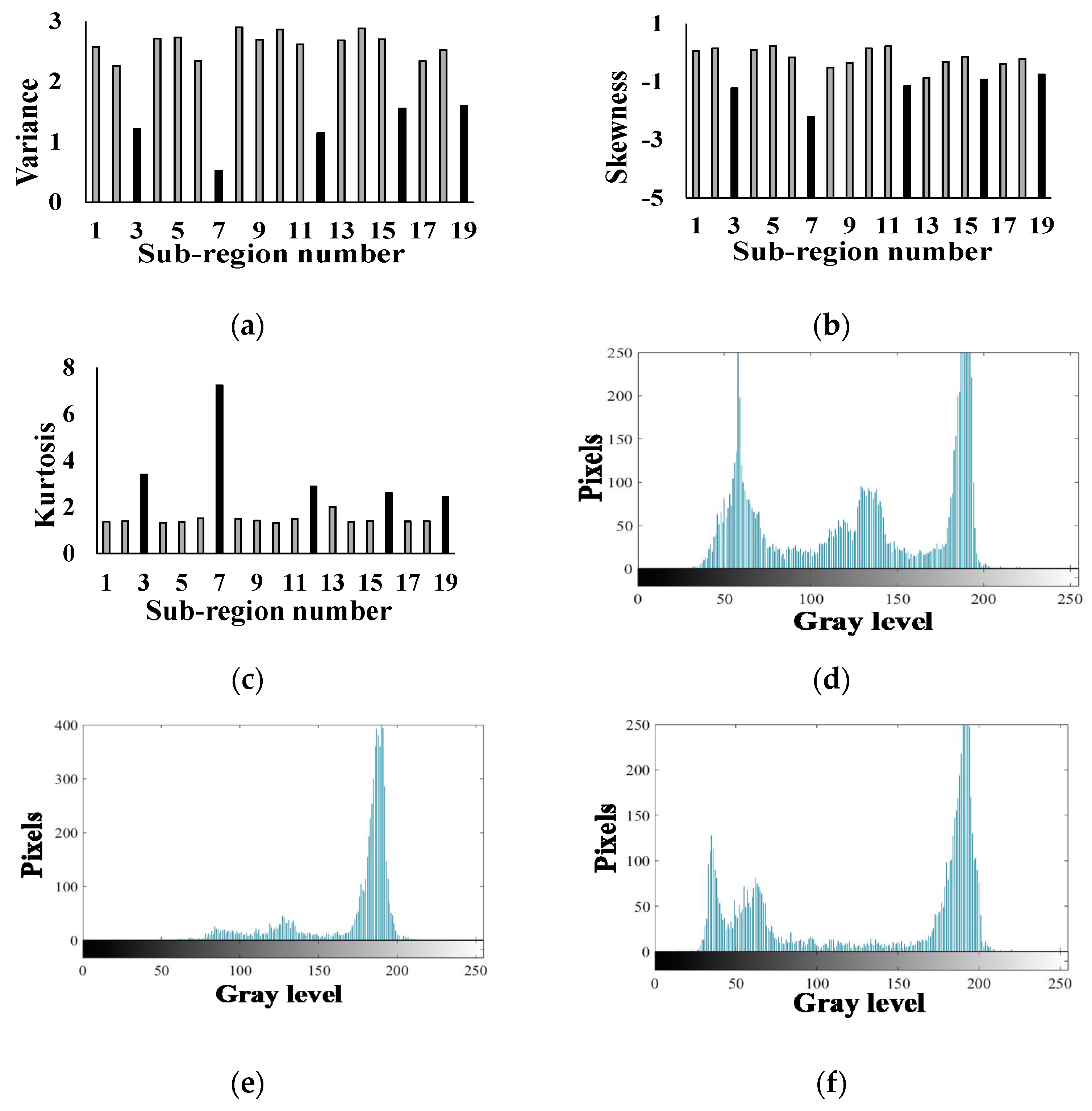
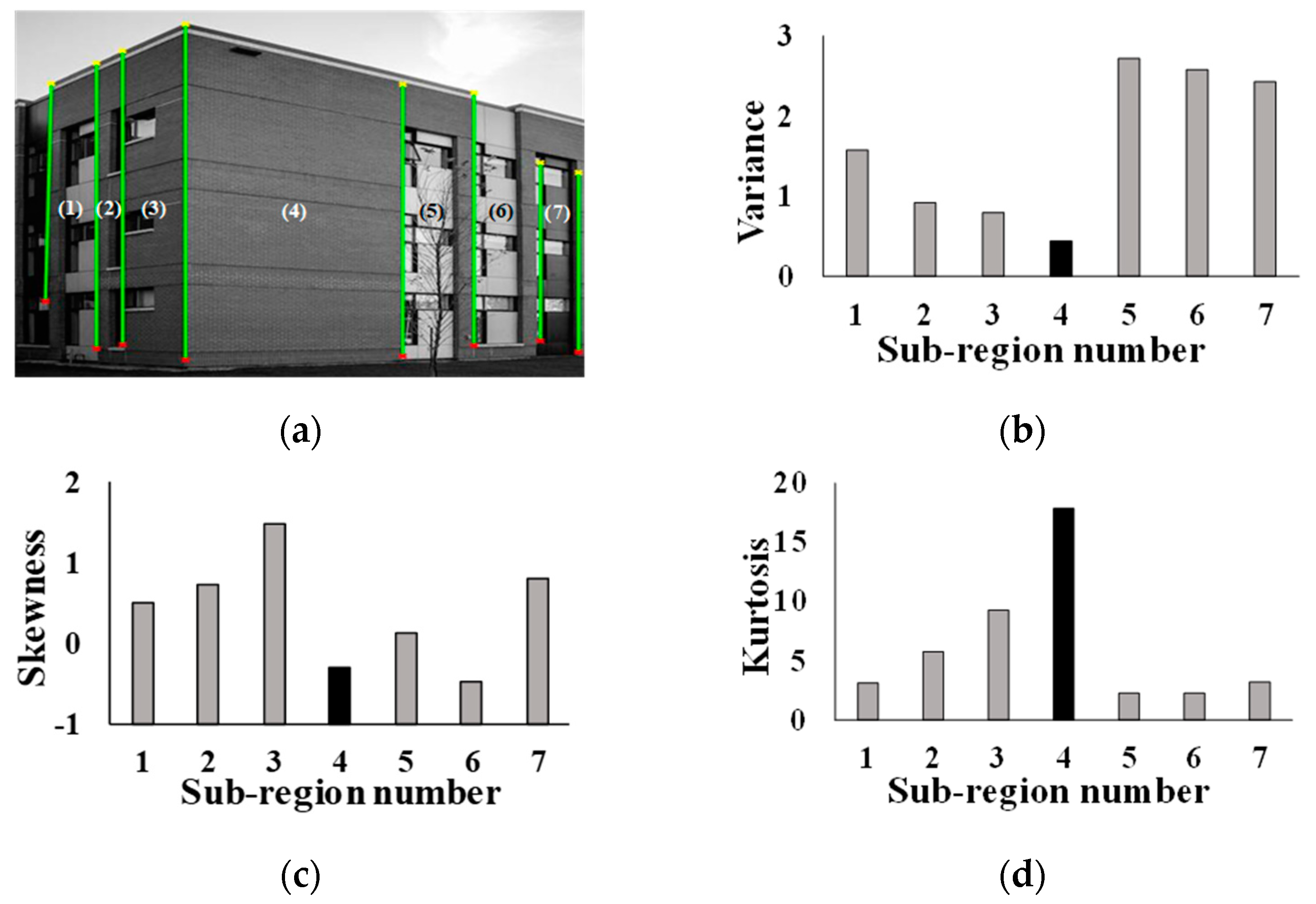
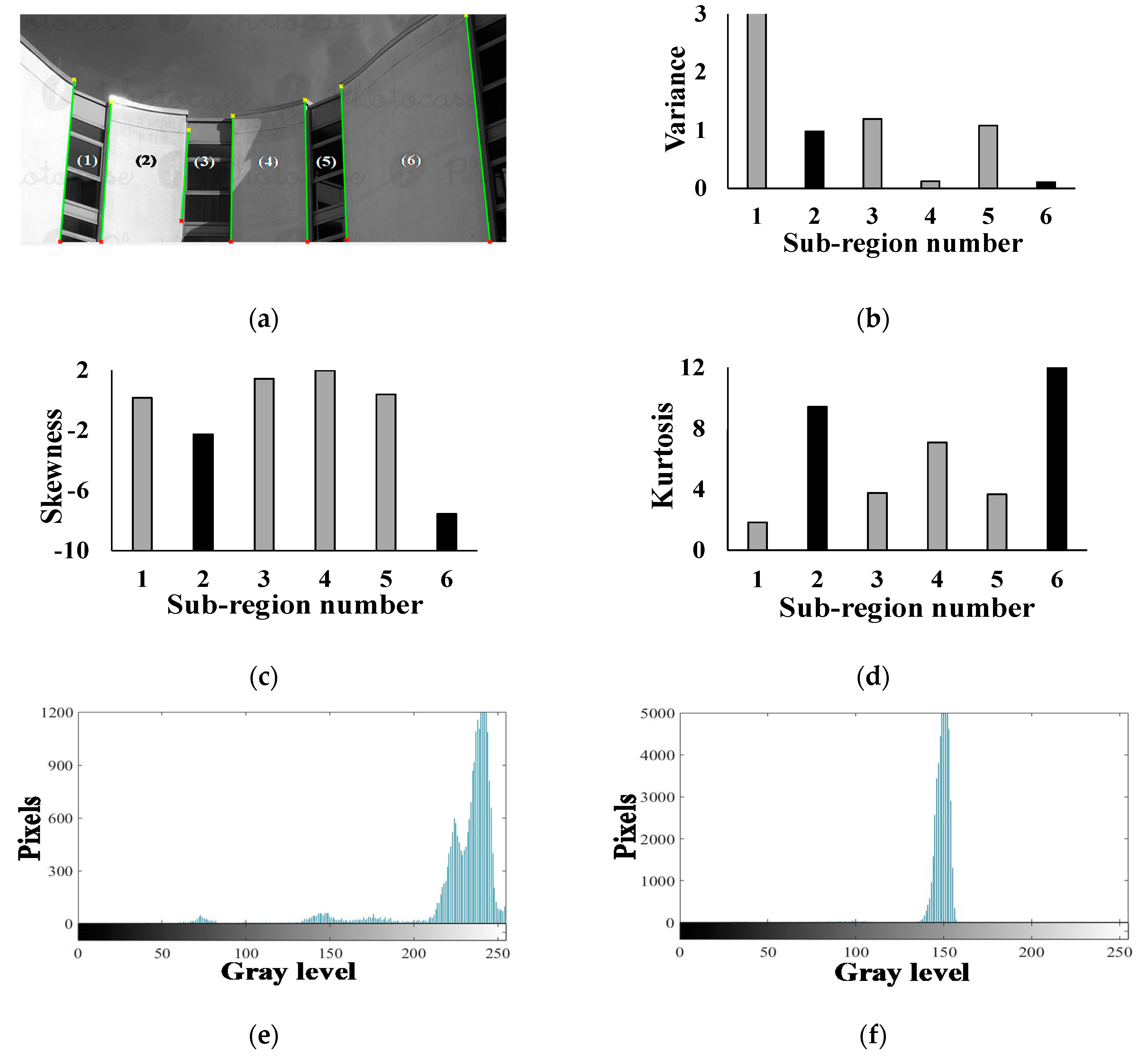
3.2. Columns and Walls Recognition using GLH Statistical Parameters

The GLH is innovatively used in this proposed study to recognize structural elements from detected sub-regions in an image. The meanings of the five GLH statistical parameters are described as follows: mean is the average gray value of a GLH; integrated density is the sum of the gray values of a GLH; variance indicates the degree of spread from the mean of a GLH; skewness represents the dissymmetric degree of the distribution of a GLH; and kurtosis reflects the tailedness of the distribution of a GLH.

By investigating GLHs of detected sub-regions, the authors found that, comparing with the GLH of the adjacent sub-regions that contain various objects, the GLH of a structural element sub-region showed a more concentrated, symmetric distribution with fat tailedness due to relatively uniform gray levels on the surface of the element (also discussed in Section 4.2.1), while differences of the gray values between structural element regions and nonstructural element regions are inconspicuous. Therefore, only variance, skewness, and kurtosis are used to differentiate GLHs between structural element sub-regions and nonstructural element sub-regions. These three statistical parameters of a GLH can be calculated by Equations (8)–(13):

$$H\left(i\right)=\frac{n_i}{m\times n},i=0,1,2,\dots ,L-1,$$

(8)

$$\mu ={{\displaystyle \sum }}_{i=0}^{L-1}i\times H\left(i\right),i=0,1,2,\dots ,L-1,$$

(9)

$$\sigma ={\left[{\displaystyle \sum }_{i=0}^{L-1}{\left(i-\mu \right)}^{2}H\left(i\right)\right]}^{1/2},$$

(10)

$$\mathrm{Variance}={{\displaystyle \sum }}_{i=0}^{L-1}{\left(i-\mu \right)}^{2}H\left(i\right),$$

(11)

$$\mathrm{Skewness}=\frac{1}{{\sigma }^3}{\displaystyle \sum }_{i=0}^{L-1}{\left(i-\mu \right)}^{3}H\left(i\right),$$

(12)

$$\mathrm{Kurtosis}=\frac{1}{{\sigma }^4}{{\displaystyle \sum }}_{i=0}^{L-1}{\left(i-\mu \right)}^{4}H\left(i\right),$$

(13)

where $i$ is the gray level of a pixel ranging from 0 to 255;$H\left(i\right)$ is the proportion of pixels in the gray level$i$; $n_i$ is the number of pixels in the gray level$i$ of a sub-region; and $m$ and $n$ are the numbers of pixels in the rows and columns of a sub-region, respectively; $\mu$ is the average gray level of pixels; $\sigma$ is the standard deviation of pixels’ gray levels; $L$ is the RGB color space, which is equal to 256. Accordingly, three GLH statistical parameters of every sub-region are calculated.

Based on the preliminary study, the authors conclude that (1) the variance and skewness values of a sub-region that is a structural element is smaller than the values of adjacent sub-regions that contain complex surrounding environment, respectively; (2) the kurtosis value of a sub-region that is a structural element is larger than the kurtosis values of adjacent sub-regions that contain complex surrounding environment. The first conclusion can be explained by the concentrated distributions of the gray levels of structural element sub-regions in narrow ranges as a result of the relatively uniform color of columns’ and walls’ surfaces, while gray levels of sub-regions containing complex surrounding environment distribute in wide ranges, leading to large variance values. Meanwhile, the centralization of gray level distributions also results in the low skewness values of structural element sub-regions because the concentration of gray level distributions leads to a relatively symmetric distribution compared with the random distribution of non-structural element sub-regions’ gray levels. Finally, based on Equation (13), for a concentrated distribution, a few pixels with extreme values (i.e., the values considerably deviate from the mean value) can lead to an extreme large skewness value of a structural element sub-region. Accordingly, this study considers a sub-region as a column or a wall if it satisfies the following criteria:

(1)

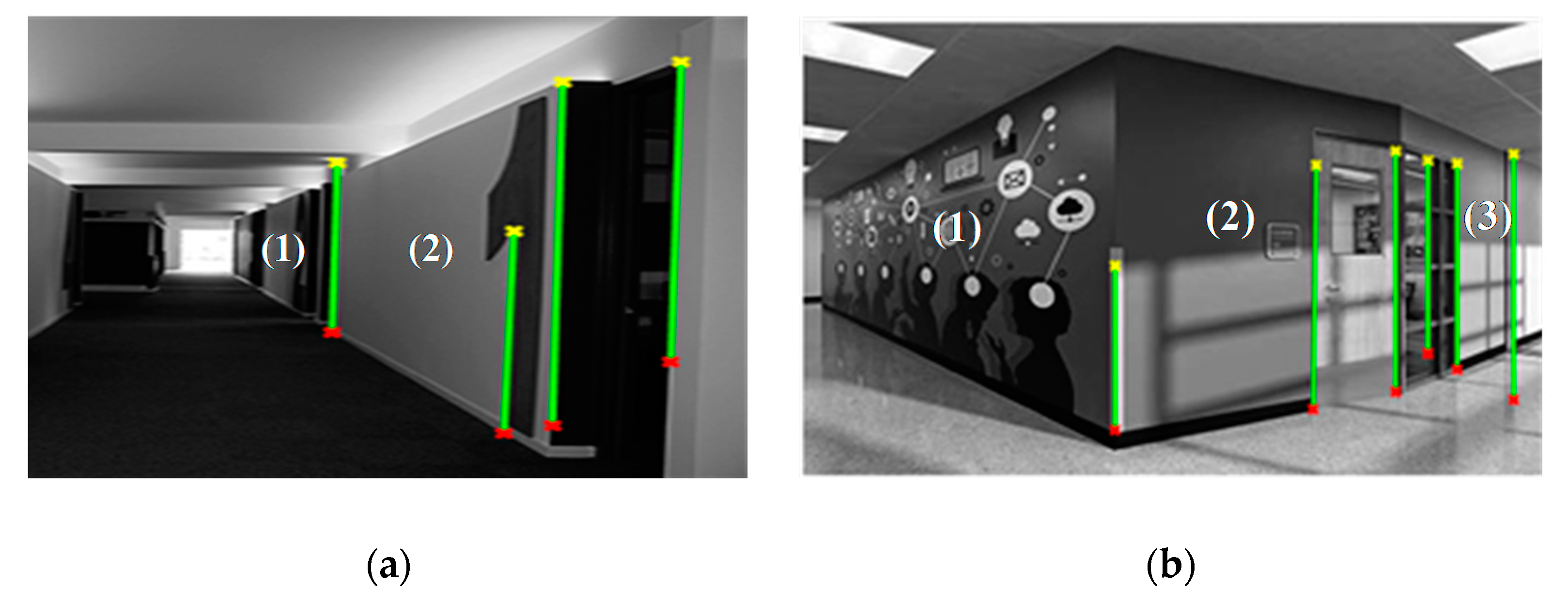
the intersection angle of a sub-region’s two adjacent boundary lines is less than 5$°$;

(2)

variance and skewness values of the sub-region’s GLH are local minimum while the kurtosis value is local maximum among adjacent sub-regions;

(3)

the ratio of length to width of a sub-region is set as no less than two for a column, and less than two for a wall. The length of a sub-region is defined by the length of its longer boundary line, and the width is defined as the distance between its two boundary lines [51].

4. Implementation and Results

4.1. Validation

The database of Taiwan’s National Center for Research on Earthquake Engineering (NCREE) contains thousands of school building images in different sizes and resolutions taken in Taiwan by various devices. The authors selected images that were taken indoors and outdoors from the front view and the side view of buildings from the database of NCREE and implemented these images in MATLAB R2017a (The MathWorks, Natick, MA, USA) to validate the performance of the proposed method. Finally, the detection precision and recall were used respectively to assess the detection accuracy and detection efficiency of the proposed method. Part of the column and wall detection results are shown in

Table 1. The column detection results for 20 column images.

Number of the Image	TP	FP	FN	Precision	Recall
				TP/(TP+FP)	TP/(TP+FN)
1	5	0	0	100.0%	100.0%
2	2	0	2	100.0%	50.0%
3	2	0	0	100.0%	100.0%
4	5	0	1	100.0%	83.3%
5	5	0	2	100.0%	71.4%
6	1	0	1	100.0%	50.0%
7	4	0	1	100.0%	80.0%
8	4	0	2	100.0%	66.7%
9	4	0	1	100.0%	80.0%
10	6	0	0	100.0%	100.0%
11	4	0	0	100.0%	100.0%
12	6	0	0	100.0%	100.0%
13	6	0	3	100.0%	66.7%
14	4	0	4	100.0%	50.0%
15	3	0	1	100.0%	75.0%
16	3	0	1	100.0%	75.0%
17	2	0	0	100.0%	100.0%
18	2	0	2	100.0%	50.0%
19	6	0	0	100.0%	100.0%
20	2	0	0	100.0%	100.0%
Total	76	0	21	100.0%	78.4%

and

Table 2. The wall detection results for 20 wall images.

Number of the Image	TP	FP	FN	Precision	Recall
				TP/(TP+FP)	TP/(TP+FN)
1	1	0	0	100.0%	100.0%
2	2	0	1	100.0%	66.7%
3	1	0	1	100.0%	50.0%
4	2	0	0	100.0%	100.0%
5	1	0	1	100.0%	50.0%
6	1	0	0	100.0%	100.0%
7	2	0	1	100.0%	66.7%
8	1	0	0	100.0%	100.0%
9	1	0	1	100.0%	50.0%
10	1	0	0	100.0%	100.0%
11	1	0	1	100.0%	50.0%
12	1	0	0	100.0%	100.0%
13	2	0	1	100.0%	66.6%
14	1	0	1	100.0%	50.0%
15	3	0	1	100.0%	75.0%
16	2	0	0	100.0%	100.0%
17	1	0	0	100.0%	100.0%
18	1	0	1	100.0%	50.0%
19	3	0	0	100.0%	100.0%
20	2	0	1	100.0%	66.7%
Total	30	0	11	100.0%	73.2%

respectively. Precision and recall are calculated by Equations (14) and (15), respectively:

$$Precision=\frac{TP}{TP+FP},$$

(14)

$$Recall=\frac{TP}{TP+FN},$$

(15)

where $TP$ (true positive) is the number of target objects (i.e., columns or walls in this study) that are correctly detected; $FP$ (false positive) is the number of detected objects that are not target objects; $FN$ (false negative) is the number of target objects that are undetected; $\left(TP+FP\right)$ is the total number of objects that are detected; $\left(TP+FN\right)$ is the total number of target objects to be detected. The values of $TP,FP,$ and $FN$ are judged manually from detection results. High precision means that most detected elements are target elements, and high recall indicates that most target elements in images are correctly detected.

4.2. Implementation and Discussion

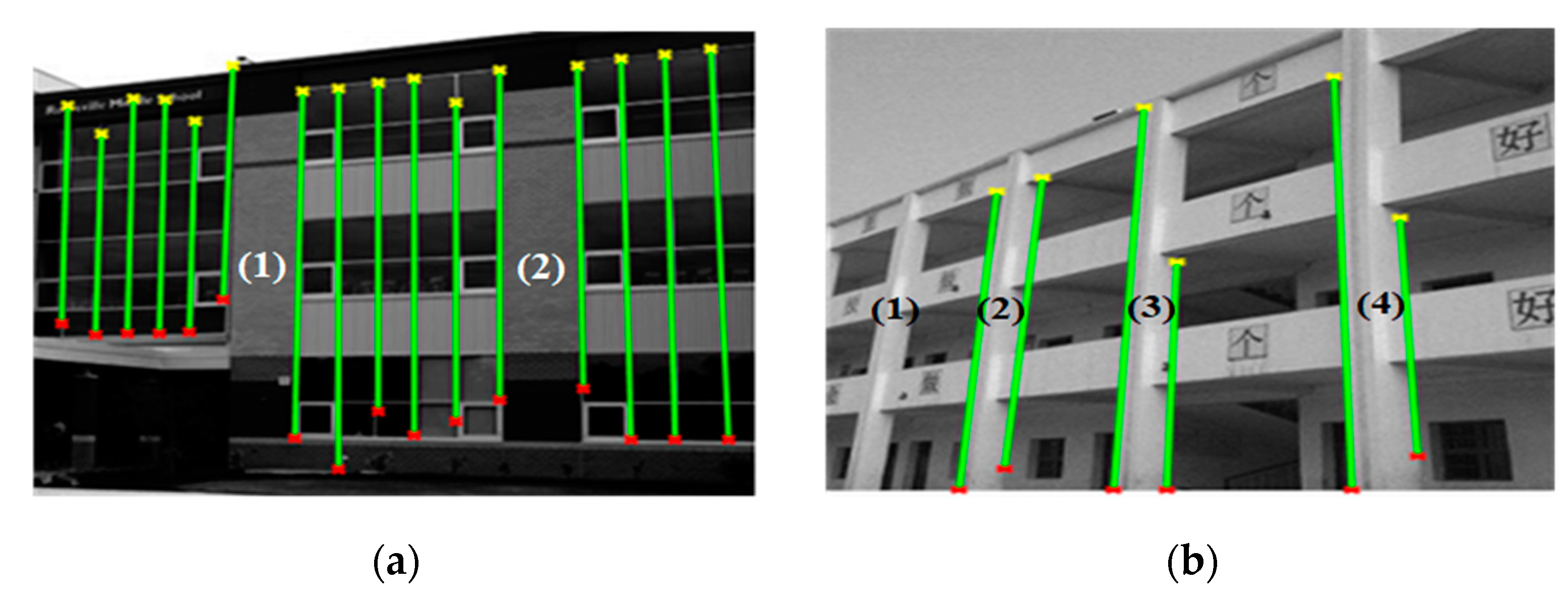
4.2.1. Column Detection Results and Discussion

The detection precision for all 20 column images in Table 1 is 100%, while detection recall ranges from 50% to 100% with an average of 78.4%. The No. 1 column image, in which all five columns were correctly detected, is taken as an example to explain the whole procedure of the proposed method. Firstly, by using Equation (1), the original RGB image (Figure 2a) was converted into a grayscale image (Figure 2b), which served as the basis of edge detection. Then, discrete edge points were detected using the Prewitt Operator, generating the edge map. As shown in Figure 2c, the edge map is a binary image in which white points are edge points and black points are the background. Next, long vertical lines, potentially to be boundaries of structural elements, were retrieved by the Hough Transform from the edge map. In this study, the authors defined a vertical line whose length is longer than a quarter of the height of the image as a long vertical line. Moreover, slightly inclined lines could also be retrieved by setting the allowed inclination of $\pm$5$°$ with the vertical direction. Consequently, 20 vertical boundary lines were detected, dividing the image into 19 sub-regions, as shown in Figure 2d. Accordingly, the variance, skewness, and kurtosis of the GLHs of every sub-regions were calculated, and sub-regions with variance and skewness values being local minimum and kurtosis values being local maximum were identified as structural elements. Finally, these detected structural elements were regarded as columns because their ratios of length to width were no less than two. As shown in Figure 3a–c, sub-region 3, 7, 12, 16, 19 are columns. It can be observed that non-column sub-regions contain various objects in different gray levels: windows in high gray levels and retaining walls in low gray levels, while column sub-regions only contain columns in similar gray levels. To further illustrate the differences of variance, skewness, and kurtosis among a column sub-region and its two adjacent non-column sub-regions, the GLHs of the column sub-region 7 and the two adjacent non-column sub-region 6 and 8 in Figure 2d are shown in Figure 3d–f respectively. Three peaks exist in Figure 3d,f but only one peak in Figure 3e, which means that in non-column sub-region 6 and 8, gray levels of pixels dispersedly distribute in wide ranges while in the column sub-region 7, gray levels of pixels concentrate on a narrow range. Therefore, compared with the GLH of adjacent non-column sub-regions, the GLH of a column sub-region shows a more concentrated and symmetric distribution, with fat tailedness.

The column detection results prove that columns with tiled or painted surfaces can be detected, overcoming the shortage of color/texture-based methods. For example, in Figure 4a, both column 1 and column 2 were successfully detected although they are tiled with colorful tiles—the top and bottom parts are tiled with dark tiles while the middle parts with light tiles. Moreover, columns with a small tilt, which commonly occur due to camera tilting or perspective illusion, can be detected by this method. As shown in Figure 4b, three tilted columns (column 2, 3 and 4) in the image, with tilt angles between their boundary lines and the vertical direction ranging from $1°$ to $5°$, were detected as a result of the maximum allowed tilt angle set as $5°$ in this study. On the other hand, taking images from the side view of structural elements can aggravate tilting of distant objects in images, leading to the failure detection of distant columns: the most distant column 1 in Figure 4b failed to be detected because the aggravated inclination of its boundary lines exceeds $5°$. To avoid such deficiency, images should be taken from the front view of structural elements.

4.2.2. Wall detection results and discussion

As shown in Table 2, similar to column detection results, the detection precision of all 20 wall images are 100% and the detection recall ranges from 50% to 100% with the average of 73.2%, proving the outstanding capability of the proposed method in correctly detecting columns and walls. Looking into these images, the authors found that the proposed method was able to detect structural elements in complex scenarios. Take the No. 1 image in Table 2 as an example. Compared with the similar GLHs among non-column sub-regions (Figure 3), GLHs are markedly different from each other among non-column sub-regions in Figure 5a, leading to the huge differences of variance, skewness and kurtosis values among non-column sub-regions. The variance value in the sub-region 2 is much smaller than the value in the sub-region 6 (Figure 5b,c) while the skewness value in the sub-region 2 is much bigger than the value in the sub-region 6 (Figure 5d). However, most sub-regions with complex scenarios in wall images have little influence on the detection results because only these sub-regions adjacent to structural element sub-regions can determine the detection results of structural elements. As shown in Figure 5, whether the wall in sub-region 4 could be successfully detected is only affected by adjacent sub-region 3 and 5 in spite of other sub-regions with diverse GLHs. Moreover, the proposed detection method is able to detect slightly distorted structural elements by setting an allowed intersection angles (5$°$) of objects’ two vertical boundary lines, compared with existing structural element detection methods which assume that the vertical boundaries of a structural element are a pair of parallel lines [28]. For instance, the wall (sub-region 4) in Figure 5a were successfully detected even if its two boundary lines are not parallel with an intersection angle of $2°$ caused by perspective illusion. On the other hand, the perspective illusion can lead to the failure detection of distant structure elements in images whose boundary lines are too blurry to be detected. For instance, wall 1 in Figure 6a and wall 1 in Figure 6b were not successfully detected because the edge detection method was unable to retrieve these walls’ left boundary lines that are invisible due to far distance between the walls and the camera–perspective illusion makes distant object small and blurry. Therefore, images that are taken from the side view of the structural elements to be detected result in low detection recall.

Another advantage of the presented method is that different illumination intensities in images will not hinder structural elements from being successfully detected. The change in illumination intensities can only result in translation motion of GLHs: the peaks of GLHs move to high gray level side under high illumination and move to low gray level side under low illumination, without changing their concentration, symmetry, and tailedness. As shown in Figure 7, gray levels of pixels in light sub-region 2 mainly range from 200 to 250 while gray levels of pixels in dark sub-region 6 are mainly around 150. However, the shapes of these two GLHs show fewer differences. The insensitivity to illumination intensity of this method allows images to be collected throughout the daytime, overcoming the limitation of traditional image recognition methods that images should be collected in the same time period of a day (Han et al. 2017). On the other hand, the non-uniform illumination on the surface of an element can result in failure of detection due to the asymmetric distribution of the element’s GLH. For instance, the wall 4 in Figure 7a, with non-uniform illumination on its surface, failed to be detected because of the local maximum value of the skewness in sub-region 4 (Figure 7c). Thus, non-uniform illumination on surfaces of structural elements should be avoided when taking photos.

5. Conclusions

Realizing the benefits of collecting building information using visual data, researchers have begun to focus on the automatic extraction of structural characteristics from images to quickly assess seismic vulnerabilities of regional-scale buildings. However, existing structural element detection methods have a certain of limitations for the detection of school building columns and walls. To improve existing automatic structural element detection techniques, this paper combines the GLH statistical feature-based object-detection method with an improved shape-based method: the former can identify structural elements from complex scenarios, and the latter has proved its superior capability in detecting slant objects in an image. Focusing on detecting columns and walls, the proposed method was validated by testing the detection precision and recall for column and wall images selected from the database of NCREE, respectively. The main advantages of the proposed column and wall detection method are listed as follows. First, the present method is able to detect columns and walls with various surface treatments or slightly tilting shapes which frequently occur in images. Second, images in different sizes and resolutions taken by either cameras or mobile phones can be used in this method, broadening the sources and decreasing the cost for images collection. Last, the proposed method is insensitive to illumination intensities which means that images taken in different time periods of a day can be used in this method. As three GLH statistical parameters used in this method only depend on the shapes of GLHs, their values are insusceptible of the average high or low illumination intensities. On the other hand, as for the unsuccessful detection of columns and walls, the main reason is that images are not taken from the front view of structural elements. Camera tilting and perspective illusion can aggravate the inclination of distant elements, leading to the failure of detecting their boundary lines. Therefore, taking images from the front view of the target structural elements are recommended.

Although the proposed method was applied here to only detecting and counting columns and walls, it can be further extended to detect other structural characteristics, such as sizes and surface defects of structural elements, or structural deficiencies, such as short columns and soft-stories, as broader applications to automatically extract structural information from digital images. Furthermore, as glass has been widely used for facades in modern buildings and the failure of such glass-elements can lead to serious casualties in earthquakes, automatic detection of building elements made of glass is a critical and challenging issue in the future [52]. The proposed GLH statistical feature-based object-detection method has the potential for solving such issue because the gray levels of glass-elements’ surfaces are homogeneous compared with the gray levels of surrounding environment that contains various objects, while the color/texture-based methods may fail to work in detecting glass that has various colors and surface treatments.

References

1. Zhang, Z.; Hsu, T.-Y.; Wei, H.-H.; Chen, J.-H. Development of a Data-Mining Technique for Regional-Scale Evaluation of Building Seismic Vulnerability. Appl. Sci. 2019, 9, 1502. [Google Scholar] [CrossRef]
2. Zhong, L.-L.; Lin, K.-W.; Su, G.-L.; Huang, S.-J.; Wu, L.-Y. Primary assessment and statistical analysis for the seismic resistance ability of middle school buildings. Struct. Eng. 2012, 27, 61–81. [Google Scholar]
3. Ploeger, S.; Sawada, M.; Elsabbagh, A.; Saatcioglu, M.; Nastev, M.; Rosetti, E. Urban RAT: New tool for virtual and site-specific mobile rapid data collection for seismic risk assessment. J. Comput. Civ. Eng. 2015, 30, 04015006. [Google Scholar] [CrossRef]
4. Ye, S.; Zhu, D.; Yao, X.; Zhang, X.; Li, L. Developing a mobile GIS-based component to collect field data. In Proceedings of the International Conference on Agro-Geoinformatics, Tianjin, China, 18–20 July 2016; pp. 1–6. [Google Scholar]
5. Mayer, H. Automatic object extraction from aerial imagery—A survey focusing on buildings. Comput. Vis. Image Underst. 1999, 74, 138–149. [Google Scholar] [CrossRef]
6. Lee, S.C.; Nevatia, R. Extraction and integration of window in a 3D building model from ground view images. In Proceedings of the 2004 IEEE Computer on Computer Vision and Pattern Recognition, Washington, DC, USA, 27 June–2 July 2004. [Google Scholar]
7. Zhu, Z.; Brilakis, I. Automated detection of concrete columns from visual data. In Proceedings of the Computing in Civil Engineering, Austin, TX, USA, 24–27 June 2009; pp. 135–145. [Google Scholar]
8. Li, Z.; Liu, Z.; Shi, W. A fast level set algorithm for building roof recognition from high spatial resolution panchromatic images. Geosci. Remote Sens. Lett. 2014, 11, 743–747. [Google Scholar]
9. Wu, H.; Cheng, Z.; Shi, W.; Miao, Z.; Xu, C. An object-based image analysis for building seismic vulnerability assessment using high-resolution remote sensing imagery. Nat. Hazards 2014, 71, 151–174. [Google Scholar] [CrossRef]
10. Koch, C.; Georgieva, K.; Kasireddy, V.; Akinci, B.; Fieguth, P. A review on computer vision based defect detection and condition assessment of concrete and asphalt civil infrastructure. Adv. Eng. Inform. 2015, 29, 196–210. [Google Scholar] [CrossRef] [Green Version]
11. Liang, X. Image-based post-disaster inspection of reinforced concrete bridge systems using deep learning with Bayesian optimization. Comput.-Aided Civ. Infrastruct. Eng. 2019, 34, 415–430. [Google Scholar] [CrossRef]
12. Koch, C.; Paal, S.G.; Rashidi, A.; Zhu, Z.; König, M.; Brilakis, I. Achievements and challenges in machine vision-based inspection of large concrete structures. Adv. Struct. Eng. 2014, 17, 303–318. [Google Scholar] [CrossRef]
13. German, S.; Jeon, J.-S.; Zhu, Z.; Bearman, C.; Brilakis, I.; DesRoches, R.; Lowes, L. Machine vision-enhanced postearthquake inspection. J. Comput. Civ. Eng. 2013, 27, 622–634. [Google Scholar] [CrossRef]
14. Mansour, A.K.; Romdhane, N.B.; Boukadi, N. An inventory of buildings in the city of Tunis and an assessment of their vulnerability. Bull. Earthq. Eng. 2013, 11, 1563–1583. [Google Scholar] [CrossRef]
15. Riedel, I.; Guéguen, P.; Dalla Mura, M.; Pathier, E.; Leduc, T.; Chanussot, J. Seismic vulnerability assessment of urban environments in moderate-to-low seismic hazard regions using association rule learning and support vector machine methods. Nat. Hazards 2015, 76, 1111–1141. [Google Scholar] [CrossRef]
16. Dimitrov, A.; Golparvar-Fard, M. Vision-based material recognition for automated monitoring of construction progress and generating building information modeling from unordered site image collections. Adv. Eng. Inform. 2014, 28, 37–49. [Google Scholar] [CrossRef]
17. Abeid Neto, J.; Arditi, D.; Evens, M.W. Using colors to detect structural components in digital pictures. Comput. Aided Civ. Infrastruct. Eng. 2002, 17, 61–67. [Google Scholar] [CrossRef]
18. Brilakis, I.K.; Soibelman, L. Shape-based retrieval of construction site photographs. J. Comput. Civ. Eng. 2008, 22, 14–20. [Google Scholar] [CrossRef]
19. Luo, H.; Paal, S.G. Machine learning–based backbone curve model of reinforced concrete columns subjected to cyclic loading reversals. J. Comput. Civ. Eng. 2018, 32, 04018042. [Google Scholar] [CrossRef]
20. DeGol, J.; Golparvar-Fard, M.; Hoiem, D. Geometry-Informed Material Recognition. In Proceedings of the Conference on Computer Vision and Pattern Recognition, Las Vegas, NV, USA, 26 June–1 July 2016; pp. 1554–1562. [Google Scholar]
21. Rashidi, A.; Sigari, M.H.; Maghiar, M.; Citrin, D. An analogy between various machine-learning techniques for detecting construction materials in digital images. KSCE J. Civ. Eng. 2016, 20, 1178–1188. [Google Scholar] [CrossRef]
22. Han, K.; Degol, J.; Golparvar-Fard, M. Geometry-and Appearance-Based Reasoning of Construction Progress Monitoring. J. Constr. Eng. Manag. 2017, 144, 04017110. [Google Scholar] [CrossRef]
23. Park, M.-W.; Brilakis, I. Construction worker detection in video frames for initializing vision trackers. Autom. Constr. 2012, 28, 15–25. [Google Scholar] [CrossRef]
24. Wiebel, C.B.; Valsecchi, M.; Gegenfurtner, K.R. The speed and accuracy of material recognition in natural images. Atten. Percept. Psychophys. 2013, 75, 954–966. [Google Scholar] [CrossRef] [Green Version]
25. Cimpoi, M.; Maji, S.; Vedaldi, A. Deep filter banks for texture recognition and segmentation. In Proceedings of the 2015 IEEE Conference on Computer Vision and Pattern Recognition (CVPR), Boston, MA, USA, 7–12 June 2015; pp. 3828–3836. [Google Scholar]
26. Jung, C.R.; Schramm, R. Rectangle detection based on a windowed Hough transform. In Proceedings of the Brazilian Symposium on Computer Graphics and Image, Curitiba, Brazil, 20 October 2004; pp. 113–120. [Google Scholar]
27. Zingman, I.; Saupe, D.; Lambers, K. Automated search for livestock enclosures of rectangular shape in remotely sensed imagery. In Proceedings of the SPIE Remote Sensing, Dresden, Germany, 23–26 September 2013; p. 88920F. [Google Scholar]
28. Zhu, Z.; Brilakis, I. Concrete column recognition in images and videos. J. Comput. Civ. Eng. 2010, 24, 478–487. [Google Scholar] [CrossRef]
29. Zhang, Y.; Huo, L.; Li, H. Automated Recognition of a Wall between Windows from a Single Image. J. Sens. 2017, 2017, 1–8. [Google Scholar] [CrossRef] [Green Version]
30. Hamledari, H.; McCabe, B.; Davari, S. Automated computer vision-based detection of components of under-construction indoor partitions. Autom. Constr. 2017, 74, 78–94. [Google Scholar] [CrossRef]
31. Haralick, R.M.; Shanmugam, K. Textural features for image classification. Trans. Syst. Man Cybern. 1973, 6, 610–621. [Google Scholar] [CrossRef]
32. Jobanputra, R.; Clausi, D.A. Texture analysis using Gaussian weighted grey level co-occurrence probabilities. In Proceedings of the Conference on Computer and Robot Vision, London, ON, Canada, 17–19 May 2004; pp. 51–57. [Google Scholar]
33. Liu, H.; Guo, H.; Zhang, L. SVM-based sea ice classification using textural features and concentration from RADARSAT-2 Dual-Pol ScanSAR data. IEEE J. Sel. Top. Appl. Earth Obs. Remote Sens. 2015, 8, 1601–1613. [Google Scholar] [CrossRef]
34. Zhu, T.; Li, F.; Heygster, G.; Zhang, S. Antarctic Sea-Ice Classification Based on Conditional Random Fields From RADARSAT-2 Dual-Polarization Satellite Images. IEEE J. Sel. Top. Appl. Earth Obs. Remote Sens. 2016, 9, 2451–2467. [Google Scholar] [CrossRef]
35. Paneque-Gálvez, J.; Mas, J.-F.; Moré, G.; Cristóbal, J.; Orta-Martínez, M.; Luz, A.C.; Guèze, M.; Macía, M.J.; Reyes-García, V. Enhanced land use/cover classification of heterogeneous tropical landscapes using support vector machines and textural homogeneity. Int. J. Appl. Earth Obs. Geoinf. 2013, 23, 372–383. [Google Scholar] [CrossRef]
36. Nawaz, S.; Dar, A.H. Hepatic lesions classification by ensemble of SVMs using statistical features based on co-occurrence matrix. In Proceedings of the International Conference on Emerging Technologies, Rawalpindi, Pakistan, 18–19 October 2008; pp. 21–26. [Google Scholar]
37. Patil, R.; Sannakki, S.; Rajpurohit, V. A Survey on Classification of Liver Diseases using Image Processing and Data Mining Techniques. Int. J. Comput. Sci. Eng. 2017, 5, 29–34. [Google Scholar]
38. Liu, Y.X.; Guo, Y.Z. Grayscale Histograms Features Extraction Using Matlab. Comput. Knowl. Technol. 2009, 5, 9032–9034. [Google Scholar]
39. Sharma, B.; Venugopalan, K. Classification of hematomas in brain CT images using neural network. In Proceedings of the International Conference on Issues and Challenges in Intelligent Computing Techniques, Ghaziabad, India, 7–8 February 2014; pp. 41–46. [Google Scholar]
40. Ozkan, E.; West, A.; Dedelow, J.A.; Chu, B.F.; Zhao, W.; Yildiz, V.O.; Otterson, G.A.; Shilo, K.; Ghosh, S.; King, M. CT gray-level texture analysis as a quantitative imaging biomarker of epidermal growth factor receptor mutation status in adenocarcinoma of the lung. Am. J. Roentgenol. 2015, 205, 1016–1025. [Google Scholar] [CrossRef]
41. Zhang, W.L.; Wang, X.Z. Feature extraction and classification for human brain CT images. In Proceedings of the International Conference on Machine Learning and Cybernetics, Hong Kong, China, 19–22 August 2007; pp. 1155–1159. [Google Scholar]
42. Fallahi, A.R.; Pooyan, M.; Khotanlou, H. A new approach for classification of human brain CT images based on morphological operations. J. Biomed. Sci. Eng. 2010, 3, 78–82. [Google Scholar] [CrossRef] [Green Version]
43. An, J.; Liu, H.; Pan, L.; Zhang, K. Classification of traffic signs based on fusion of PCA and gray level histogram. Highway 2017, 62, 185–197. [Google Scholar]
44. Peli, T.; Malah, D. A study of edge detection algorithms. Comput. Graph. Image Process. 1982, 20, 1–21. [Google Scholar] [CrossRef]
45. Prewitt, J.M. Object enhancement and extraction. In Picture Processing and Psychopictorics; Academic Press: London, UK, 1970; Volume 10, pp. 15–19. [Google Scholar]
46. Kanopoulos, N.; Vasanthavada, N.; Baker, R.L. Design of an image edge detection filter using the Sobel operator. J. Solid State Circuits 1988, 23, 358–367. [Google Scholar] [CrossRef]
47. Jain, R.; Kasturi, R.; Schunck, B.G. Machine Vision; McGraw-Hill: New York, NY, USA, 1995; Volume 5. [Google Scholar]
48. Canny, J. A computational approach to edge detection. Trans. Pattern Anal. Mach. Intell. 1986, 8, 679–698. [Google Scholar] [CrossRef]
49. Chaple, G.N.; Daruwala, R.; Gofane, M.S. Comparisions of Robert, Prewitt, Sobel operator based edge detection methods for real time uses on FPGA. In Proceedings of the International Conference on Technologies for Sustainable Development, Mumbai, India, 4–6 February 2015; pp. 1–4. [Google Scholar]
50. Pratt, W.K. Digital Image Processing, 3rd ed.; John Wiley & Sons, Inc.: New York, NY, USA, 2001. [Google Scholar]
51. Japan Building Disaster Prevention Association. Standard for Seismic Evaluation of Existing Reinforced Concrete Buildings; Japan Building Disaster Prevention Association: Tokyo, Japan, 2001. [Google Scholar]
52. Bedon, C.; Zhang, X.; Santos, F.; Honfi, D.; Kozłowski, M.; Arrigoni, M.; Figuli, L.; Lange, D. Performance of structural glass facades under extreme loads—Design methods, existing research, current issues and trends. Constr. Build. Mater. 2018, 163, 921–937. [Google Scholar] [CrossRef]
Figure 1. The process map for the automatic detection of columns and walls.
Applsci 09 03915 g001
Figure 2. The preprocessing of the No. 1 image in Table 1: (a) the original image; (b) converting the RGB image into a grayscale image; (c) generating the edge map using the Prewitt Operator; (d) detecting long vertical lines by the Hough transform.
Applsci 09 03915 g002
Figure 3. Column recognition of the No. 1 image in Table 1 (sub-region 3, 7, 12, 16, and 19 are columns): (a) variance of gray-level histograms (GLHs); (b) skewness of GLHs; (c) kurtosis of GLHs; (d) the GLH in sub-region 6 (non-structural element); (e) the GLH in sub-region 7 (a column); (f) the GLH in sub-region 8 (non-structural element).
Applsci 09 03915 g003
Figure 4. Examples of column detection results: (a) the No. 3 image in Table 1; (b) the No. 16 image in Table 1.
Applsci 09 03915 g004
Figure 5. The wall detection result of the No. 1 image in Table 2 (the sub-region 4 is a wall): (a) the preprocessed image; (b) variance of GLHs; (c) skewness of GLHs; (d) kurtosis of GLHs.
Applsci 09 03915 g005
Figure 6. The wall detection results: (a) the No. 3 image in Table 2, (b) the No. 7 image in Table 2.
Applsci 09 03915 g006
Figure 7. The wall detection result of the No. 13 image in Table 2 (sub-region 2, 4, and 6 contain walls while only walls in sub-region 2 and 6 are detected): (a) the preprocessed image; (b) variance of GLHs; (c) skewness of GLHs; (d) kurtosis of GLHs; (e) the GLH in sub-region 2 (a wall); (f) the GLH in sub-region 6 (a wall).
Applsci 09 03915 g007