A Novel Genetic Algorithm for the Synthetical Sensor-Weapon-Target Assignment Problem

Abstract

The sensor-weapon–target assignment (S-WTA) problem is a crucial decision issue in C4ISR. The cooperative engagement capability (CEC) of sensors and weapons depends on the S-WTA schemes, which can greatly affect the operational effectiveness. In this paper, a mathematical model based on the synthetical framework of the S-WTA problem is established, combining the dependent and independent cooperative engagement modes of sensors and weapons. As this problem is a complex combinatorial optimization problem, a novel genetic algorithm is proposed to improve the solution of this formulated S-WTA model. Based on the prior knowledge of this problem, a problem-specific population initialization method and two novel repair operators are introduced. The performances of the proposed algorithm have been validated on the known benchmarks. Extensive experimental studies compared with three state-of-the-art approaches demonstrate that the proposed algorithm can generate better assignment schemes for the most of the benchmarks.

1. Introduction

The sensor-weapon–target assignment (S-WTA) problem, as one of the most important issues in C4ISR [1,2], has attracted great attention in recent years. Its objective is to find an appropriate assignment scheme for sensors and weapons to enemy targets with the goal of maximizing the benefit of the scheme. This problem is a constrained combinatorial optimization problem, which can be regarded as a nondeterministic polynomial time complete (NP-complete) problem [3]. For certain cases, S-WTA can be considered as a composite of two independent parts, i.e., the sensor–target assignment (STA) [4,5,6,7,8] and the weapon–target assignment (WTA) [9,10,11,12,13,14,15,16]. As the sensor is mainly used to obtain the information of the battlefield situation, the STA is performed in the mission of reconnaissance and surveillance to make decisions for the sensor management. As the weapon is used to protect the assets and obtain the superiority in the engagement, the WTA is implemented in the mission of attack to intercept and destroy the target. At present, as network-centric warfare (NCW) [17] and knowledge-centric warfare (KCW) [18] are the key operational architectures of the military operations, autonomy and cooperation are becoming more and more important. As a result, in this paper, we focus on the S-WTA problem, in which the sensors and weapons are allocated cooperatively. To be specific, the sensor can transmit the target information to the weapon in real-time and guide the weapon to attack the target accurately.

In the last few decades, some scholars have paid attention to the S-WTA problem. The S-WTA model was established by Bogdanowicz and Coleman [19] for the first time. They deeply analyzed the characteristics of the S-WTA problem and proposed two types of S-WTA models: the independent S-WTA model and the dependent S-WTA model. Meanwhile, a heuristic algorithm based on auction algorithm was put forward in their paper to solve these S-WTA models. Afterwards, based on the proposed S-WTA model, Bogdanowicz further improved the auction algorithms named as Swt-opt [20], which has been proved that Swt-opt can generate complete optimal assignment. In order to improve the efficiency of the allocation schemes over many dynamic network topologies, Li et al. [21] proposed an improved Swt-opt, combining the consensus algorithm with Swt-opt. Li et al. [22] introduced the temporal and spatial constraints into the S-WTA problem to establish an improved dependent model. They considered this specific S-WTA problem as a kind of dynamic weapon–target assignment (DWTA) [23] problem and proposed an anytime algorithm based on decentralized cooperative auction to solve this problem. Chen et al. [24] proposed an improved particle swarm optimization (PSO) to solve a similar dependent S-WTA problem. In this algorithm, some novel genetic operators were adopted to enhance the performance of the algorithm. Ezra et al. [25,26] analyzed the integrated relationship between sensor, weapon, and target. They proposed four integrated formulations combining the sensor resource management and weapon–target assignment to further demonstrate the characteristics of the independent and dependent S-WTA problem. Wang et al. [27] proposed an improved genetic algorithm (GA) to solve the dependent S-WTA problem, considering the situation where the kill probability of the weapons was modified to a formula with regard to the detection precision of sensors. Taking into account the synergic relationship between weapons and sensors as well as some specific constraints, Xin et al. [28] established a novel dependent S-WTA model. Moreover, they proposed a marginal-return-based constructive heuristic (MRBCH) to solve the formulated S-WTA model, so as to generate the allocation scheme rapidly and accurately. The work has been discussed thus far only focus on one aspect of the S-WTA problem. Consequently, some details of the collaborative operations of the sensors and weapons, which involve the cooperative engagement mode and the capacity constraints, are neglected. Therefore, in this paper, we focus on designing a comprehensive S-WTA model to demonstrate a more realistic S-WTA scenario.

In order to improve the solution of the S-WTA model, the optimization algorithm is also studied in this paper. The algorithms used to solve the S-WTA problem can be divided into two categories: The first category is the heuristic algorithm, such as Swt-opt and MRBCH. Heuristic algorithms can solve the S-WTA in real-time. It can be used in a dynamic environment and handle the uncertainties over the engagement. Although heuristic algorithms can solve the S-WTA problem in real-time, they are very difficult to achieve a satisfactory solution in such a NP-hard problem. This is because heuristic algorithms search for solutions using specific heuristic information, which traps them into the local optimal easily. The second category is the evolutionary algorithm (EA) [29,30], such as GA and PSO. As EA-based algorithms use many flexible mechanisms that fully consider the prior knowledge, they can achieve a satisfactory solution. However, the running time of EA-based algorithms are relatively large; they cannot solve the S-WTA problems in real-time. In this paper, as we focus on obtaining a high-quality assignment scheme, the running time of the algorithm is not considered. Since EA has many significant advantages in finding the optimal solution, we believe that choosing EA to solve the S-WTA problem can achieve a satisfactory assignment scheme.

EA has attracted massive interest from researchers for decades. At present, the well-known evolutionary algorithms are GA [31], PSO [32], ant colony algorithm (ACO) [33], and differential evolution (DE) [34]. Among these algorithms, GA is one of the most important algorithms. Because GA has a simple framework, high flexibility, and strong convergence ability, it has been successfully applied in many real-world problems [35,36,37], especially in the WTA problem [13,23,38]. For these reasons, we believe that choosing GA to solve the S-WTA problem is reasonable and promising. In this paper, we proposed a novel GA to solve the S-WTA problem named GA-SWTA. The contributions of this paper are described as follows.

(1)

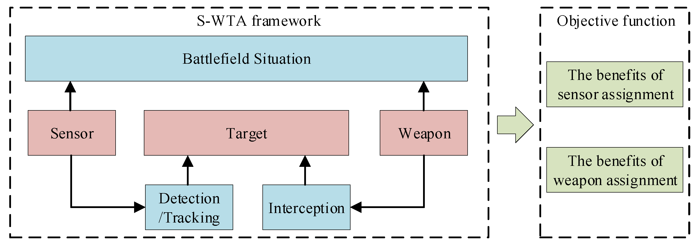
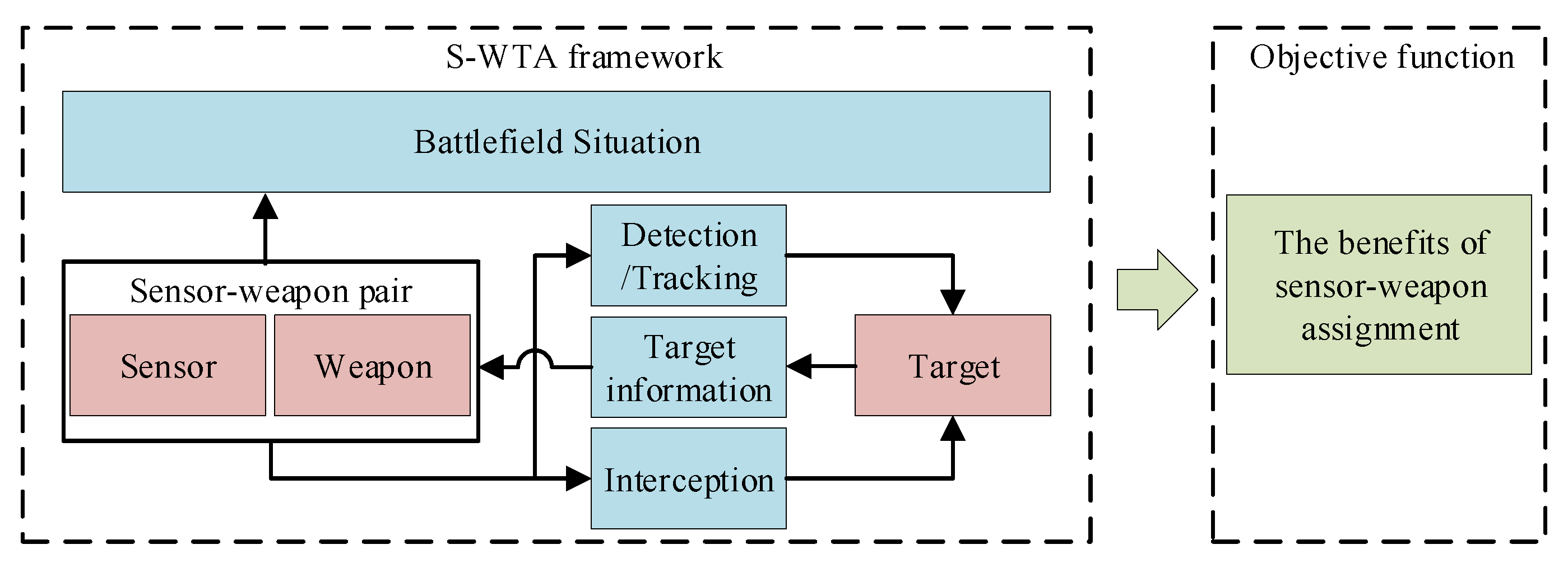
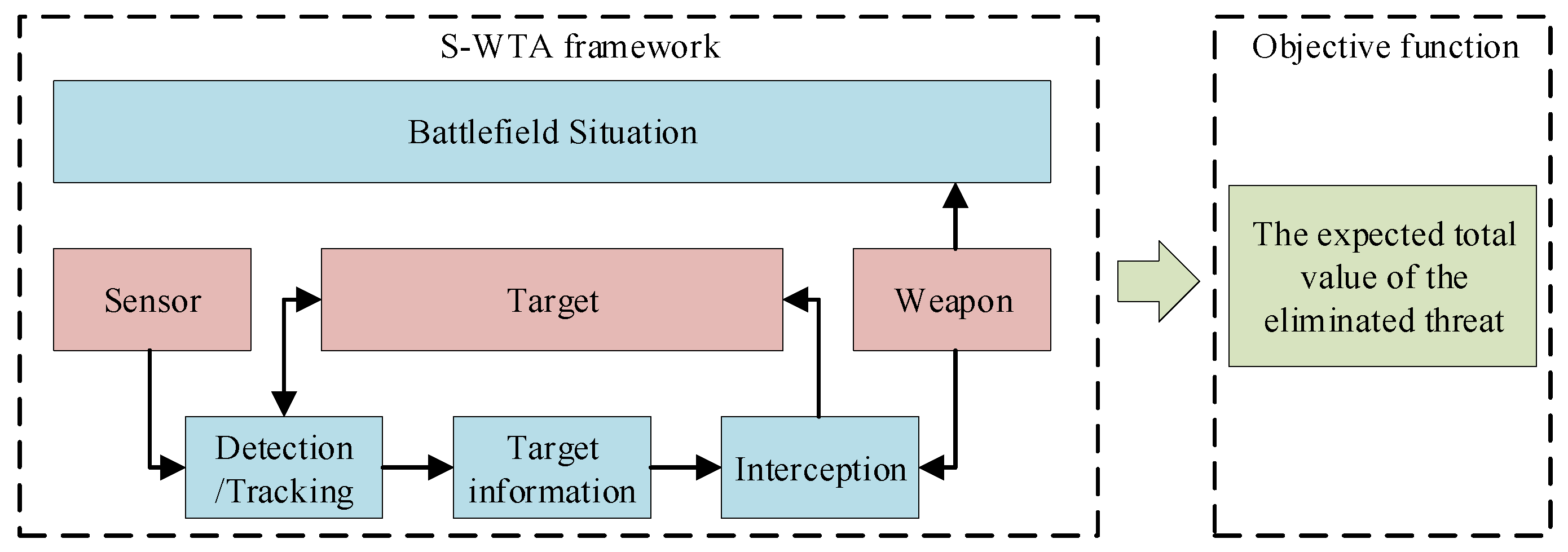
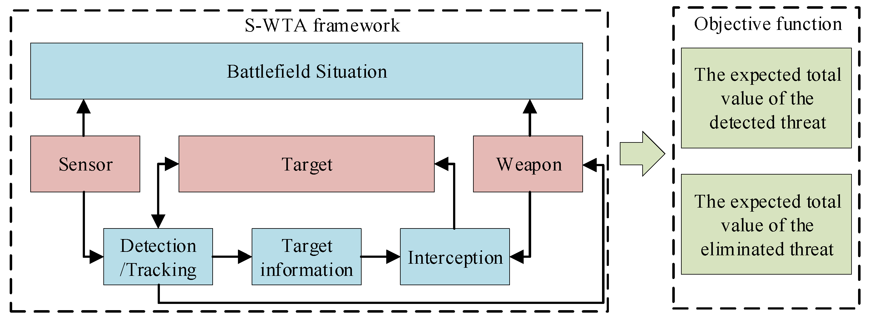
In the context that sensors and weapons are allocated cooperatively, a novel S-WTA model is presented. The traditional S-WTA model has only two frameworks: the dependent framework and the independent framework. In order to fully reflect the relationship between sensors and weapons, the S-WTA has been extended to the synthetical framework.

(2)

For the proposed S-WTA model, a novel GA framework is proposed. Based on the characteristic of S-WTA, we redefine the form of chromosome encoding. We also adaptively improved the crossover operator to better match the redefined encoding. In addition, a problem-specific chromosome initialization method is proposed.

(3)

In order to handle the constrains and improve the convergence ability of the algorithm, chromosome repair approaches are proposed. Based on the prior knowledge of S-WTA, two repair operations— R-STA operation and R-WTA operation—are designed to cooperatively repair the chromosome. The experiments validate the good performance of the proposed approaches.

The rest of this paper is organized as follows. In Section 2, the frameworks of the S-WTA problem are analyzed first, then we present a mathematical optimization model for the synthetical S-WTA problem. In Section 3, a novel GA, i.e., GA-SWTA, is proposed to solve the S-WTA problem. Meanwhile, a problem-specific initialization and a chromosome-repair mechanism are designed to improve the performance of the algorithm. In Section 4, GA-SWTA is compared with three state-of-the-art S-WTA approaches, then the performance of the proposed initialization and a chromosome-repair mechanism are investigated. The conclusion and future work are described in Section 5.

2. Problem Analysis and Formulation

2.1. Existing Work of the S-WTA Problem

In this paper, the engagement scenario is described as follows. In one engagement of a military conflict, N targets belonging to the opponent are coming under attack from the defender. The target can be any object that poses a threat to the security of the defender, such as missiles, unmanned aerial vehicles (UAVs), and so on. As each target is coming from a different direction, each one has a certain value of threat. The defender has M sensors (e.g., Doppler radar and millimeter-wave radar) to detect and track the targets. It also has W weapons (e.g., missile and antiaircraft gun) to intercept the targets.

Based on this scenario, to the best of our knowledge, there are five different formulations of the S-WTA problem. In order to present these formulations clearly, we describe these formulations with the uniform variable name. The variables used in these formulations are defined in

Table 1. Variables declaration.

$v_k$:	The threat value of the kth target.
$a_{ik}$:	The benefit of assigning ith sensor to kth target.
$b_{jk}$:	The benefit of assigning jth weapon to kth target.
$c_{i^{\prime }k}$:	The benefit of assigning $i^{\prime }$th sensor–weapon pair to kth target.
$h_{ijk}$:	The benefit of assigning ith sensor and jth weapon to kth target.
$p_{jk}$:	The kill probability that the weapon j against target k.
$q_{ik}$:	The detection and tracking probability that the sensor i against target k.
$p_{ijk}$:	The kill probability that the weapon j against target k under the detection and tracking of sensor i.
$d_{ik}$:	The sensor detection decision variable (if the ith sensor detects kth target $d_{ik}=1$; otherwise, $d_{ik}=0$).
$g_{ij}$:	The sensor guidance decision variable (if the ith sensor guides the jth weapon $g_{ij}=1$; otherwise, $g_{ij}=0$).
$x_{ik}$:	The sensor assignment decision variable (if the ith sensor is assigned to kth target $x_{ik}=1$; otherwise, $x_{ik}=0$).
$y_{jk}$:	The weapon assignment decision variable (if the jth weapon is assigned to kth target $y_{jk}=1$; otherwise, $y_{jk}=0$).
$z_{i^{\prime }k}$:	The sensor–weapon assignment decision variable (if the $i^{\prime }$th sensor–weapon pair is assigned to kth target $z_{i^{\prime }k}=1$; otherwise, $z_{i^{\prime }k}=0$, $z_{i^{\prime }k}=x_{ik}·y_{jk}$).
$u_{ijk}$:	The sensor and weapon platform assignment decision variable (if the ith sensor and jth weapon platform are assigned to kth target $u_{ijk}=1$; otherwise, $u_{ijk}=0$).

.

According to existing work of the S-WTA problem, the problem can be divided into two typical categories: independent and dependent. As the dependent model is more in line with actual engagement, most of the current models are based on the dependent model. However, the independent model has its own unique advantages. Therefore, in order to design an appropriate framework to fully describe the characteristics of the S-WTA problem, all of these models should be deeply analyzed to explore the relationship between independent and dependent S-WTA problems.

As the S-WTA problem can be categorized into the independent part and dependent part, the framework of this problem also consists of these two parts. Based on these existing formulations, we summarize these models and divide them into three frameworks: one independent framework and two dependent frameworks. The details of these frameworks are summarized as follows.

2.1.1. Framework A: The Independent S-WTA Framework

As far as we know, the mathematical models of the S-WTA problem were first proposed by Bogdanowicz and Coleman [19]. According to the benefit of the weapon assignment and sensor assignment, they proposed an independent model. The independent model is shown as

$$\left\{\begin{array}{c}max{\displaystyle \sum _{k=1}^N}{\displaystyle \sum _{i=1}^M}{a}_{ik}·x_{ik}+\max {\displaystyle \sum _{k=1}^N}{\displaystyle \sum _{j=1}^W}{b}_{jk}·y_{jk}\hfill \\ s.t.\left\{\begin{array}{c}{\displaystyle \sum _{i=1}^M}{x}_{ik}\le 1,\forall k\in \left\{1,2,\cdots ,N\right\}\hfill \\ {\displaystyle \sum _{k=1}^N}{x}_{ik}\le 1,\forall i\in \left\{1,2,\cdots ,M\right\}\hfill \\ {\displaystyle \sum _{j=1}^W}{y}_{jk}\le 1,\forall k\in \left\{1,2,\cdots ,N\right\}\hfill \\ {\displaystyle \sum _{k=1}^N}{y}_{jk}\le 1,\forall j\in \left\{1,2,\cdots ,W\right\}.\hfill \end{array}\right.\hfill \end{array}\right.$$

(1)

As shown in Equation (1), the objective function is composed of two independent parts. The first part is the total benefit of sensor assignment. The second part is the total benefit of weapon assignment. Therefore, no matter how sensors are assigned, the results of their assignment will not affect the benefit of the weapon assignment.This S-WTA model describes an independent framework. It is summarized and shown in Figure 1.

As shown in Figure 1, as the sensors and weapons are independent, the information of sensors and weapons is not shared. Furthermore, the objective function includes two parts: the benefits of sensor assignment and the benefits of weapon assignment. Therefore, the sensor assignment and the weapon assignment is directly impact on the battlefield situation. As a result, as the scheme of sensor assignment and the scheme of weapon assignment do not affect each other, their effectiveness can be clear analyzed separately. However, the relationship between sensor and weapon is neglected. Therefore, the framework is unable to provide the accurate sensor and weapon assignment scheme.

2.1.2. Framework B: The Dependent S-WTA Framework-I

In addition to the independent model, Bogdanowicz and Coleman [19] also proposed a dependent model. Equation (2) shows the dependent model. As this model is more realistic of the current engagement, it is used frequently [19,20,21].

$$max{\displaystyle \sum _{k=1}^N}{\displaystyle \sum _{i^{\prime }=1}^R}(c_{i^{\prime }k}·z_{i^{\prime }k}),$$

(2)

where R is the number of the sensor–weapon pair. In this paper, we assume that there are M sensors and W weapons, so $R=M·W$. The constraints of this formulation are the same as the model (1). As the decision variable in this model is the assignment of the sensor–weapon pair, the objective function of this formulation is the total benefit of the assignment of the sensor–weapon pair. Therefore, sensor assignment will affect the benefit of the assignment of weapons.

Li et al. [22] and Chen et al. [24] present a similar dependent S-WTA model to model (2), but reformulate the problem with a different method of calculating the benefits. The model is shown as

$$\left\{\begin{array}{c}min{\displaystyle \sum _{i=1}^M}{\displaystyle \prod _{j=1}^W}\left(1-{\displaystyle \sum _{k=1}^N}{h}_{ijk}·u_{ijk}\right)\hfill \\ s.t.\left\{\begin{array}{c}{\displaystyle \sum _{j=1}^W}{\displaystyle \sum _{k=1}^N}{u}_{ijk}=1,\forall i\in \left\{1,2,\cdots ,M\right\}\hfill \\ {\displaystyle \sum _{i=1}^M}{\displaystyle \sum _{k=1}^N}{u}_{ijk}\le n_j,\forall j\in \left\{1,2,\cdots ,W\right\}\hfill \\ {\displaystyle \sum _{i=1}^M}{\displaystyle \sum _{j=1}^W}{u}_{ijk}=m_k,\forall k\in \left\{1,2,\cdots ,N\right\},\hfill \end{array}\right.\hfill \end{array}\right.$$

(3)

where $n_j$ is the number of weapons in jth weapon platform in which all the weapons have the same kill probability to a specific target and $m_k$ is the number of weapons of intercepting kth target. As the variables and structure of model (2) and (3) are very similar, these two models can be regarded as the same kind of dependent S-WTA model.

These dependent S-WTA models describe another S-WTA framework. As we divide the existing dependent S-WTA formulations into two types, the frameworks of the dependent S-WTA models have two forms. This framework is the first form and is shown in Figure 2.

As shown in Figure 2, sensor and weapon are regarded as a unity. A sensor–weapon pair is composed by a sensor assignment scheme and a weapon assignment scheme. All the information of the sensors and weapons is shared. In addition, as the sensor assignment and weapon assignment cannot be separate in this framework, the benefits of sensor–weapon assignment are calculated in the objective function. Therefore, the sensor–weapon pair is directly impact on the battlefield situation. As a result, the sensor assignment scheme and the weapons assignment scheme are integrated entirely. The interaction between the sensor and weapon can be fully considered. However, as the sensor and weapon are too tightly coupled, the framework is unable to represent the local details about sensor and weapon.

2.1.3. Framework C: The Dependent S-WTA Framework-II

Wang et al. [27] propose another dependent S-WTA model. In this model, some complex factors are introduced, such as the detection and guidance. The formulation is described as:

$$\left\{\begin{array}{c}max{\displaystyle \sum _{k=1}^N}{v}_k·\left(1-{\displaystyle \prod _{j=1}^W}{\displaystyle \prod _{i=1}^M}\left(1-p_{ijk}·g_{ij}·d_{ik}\right)\right)\hfill \\ s.t.\left\{\begin{array}{c}{\displaystyle \sum _{i=1}^M}{\mathrm{g}}_{ij}\le 1,\forall j\in \left\{1,2,\cdots ,W\right\}\hfill \\ {\displaystyle \sum _{k=1}^N}{\mathrm{g}}_{ij}·d_{ik}\le 1,\forall i\in \left\{1,2,\cdots ,M\right\},\forall j\in \left\{1,2,\cdots ,W\right\}\hfill \\ {\displaystyle \sum _{k=1}^N}{d}_{ik}\le 1,\forall i\in \left\{1,2,\cdots ,M\right\}.\hfill \end{array}\right.\hfill \end{array}\right.$$

(4)

In addition to the above three constrains, there are another three complex constrains that indicate the conditions of the detection, guidance, and interception. The details of these constraints can be seen in the literature [27]. As the objective function of this formulation is the expected total value of the eliminated threat, this formulation is similar to the model of WTA problem. The assignment of sensors can direct influence the survivability of the target.

Xin et al. [28] take into account the detection probability of the sensors to establish the dependent S-WTA model. The model is shown as

$$\left\{\begin{array}{c}max{\displaystyle \sum _{k=1}^N}{v}_k\left(1-{\displaystyle \prod _{i=1}^M}{\left(1-q_{ik}\right)}^{x_{ik}}\right)\left(1-{\displaystyle \prod _{j=1}^W}{(1-p_{jk})}^{y_{jk}}\right)\hfill \\ s.t.\left\{\begin{array}{c}{\displaystyle \sum _{k=1}^N}{x}_{ik}\le 1,\forall i\in \left\{1,2,\cdots ,M\right\}\hfill \\ {\displaystyle \sum _{k=1}^N}{y}_{jk}\le 1,\forall j\in \left\{1,2,\cdots ,W\right\}\hfill \\ {\displaystyle \sum _{i=1}^M}{x}_{ik}\le {n^{\prime }}_k,\forall k\in \left\{1,2,\cdots ,N\right\}\hfill \\ {\displaystyle \sum _{j=1}^W}{y}_{ik}\le {m^{\prime }}_k,\forall k\in \left\{1,2,\cdots ,N\right\},\hfill \end{array}\right.\hfill \end{array}\right.$$

(5)

where $n_k^{\prime }$ is the sensor cost of target k and $m_k^{\prime }$ is the weapon cost of target k. In this model, the assignment of sensors can affect the detection probability of the target. It can fully reflect the role of sensors in the whole engagement. As the objective function is the same as Equation (4), these two models can be regarded as another same kind of dependent S-WTA model.

These S-WTA models indicate the other independent S-WTA framework. It is the second form of the dependent S-WTA models, which is summarized and shown in Figure 3.

As shown in Figure 3, sensors are assigned to detect and track the targets. Then, the information achieved by sensors is shared to the weapon. Afterwards, weapons are launched to intercept the target. Therefore, in this framework, partial information of the sensor and weapon is shared. In addition, as described in models (4) and (5), the objective functions of these formulations are the expected total value of the eliminated threat. Therefore, in this framework, only weapons can impact on the battlefield situation. As a result, since the sensor assignment schemes would affect the weapon assignment schemes, the effectiveness of weapon assignment can be fully analyzed. However, the effectiveness of weapon assignment has received so much attention that the effectiveness of sensor assignment has been neglected.

According to the above analysis, all frameworks have their own advantages and disadvantages. Because of the different frameworks focus on the different aspects of the sensor assignment and the weapon assignment, some details of the sensors and weapons are neglected. Therefore, it is necessary to design a relatively comprehensive S-WTA model and framework to fully describe the S-WTA problem.

2.2. The Improved S-WTA Model

2.2.1. The Proposed S-WTA Model

Based on the model (5), the improved S-WTA model is proposed as follows,

$$\left\{\begin{array}{c}max{\displaystyle \sum _{k=1}^N}{v}_k\left(Q_k+Q_k·P_k\right)\hfill \\ Q_k=\left(1-{\displaystyle \prod _{i=1}^M}{\left(1-q_{ik}\right)}^{x_{ik}}\right)\hfill \\ P_k=\left(1-{\displaystyle \prod _{j=1}^W}{(1-(p_{jk}+\sigma ))}^{y_{jk}}\right)\hfill \\ \sigma =\left\{\begin{array}{c}0,\mathrm{if}{\displaystyle \sum _{i=1}^M}{x}_{ik}=0\hfill \\ (1-p_{jk})·tanh({\displaystyle \sum _{i=1}^M}{x}_{ik}-1),\mathrm{if}{\displaystyle \sum _{i=1}^M}{x}_{ik}\ne 0\hfill \end{array}\right.\hfill \\ s.t.\left\{\begin{array}{c}{\displaystyle \sum _{k=1}^N}{x}_{ik}\le 1,\forall i\in \left\{1,2,\cdots ,M\right\}\hfill \\ {\displaystyle \sum _{k=1}^N}{y}_{jk}\le 1,\forall j\in \left\{1,2,\cdots ,W\right\}\hfill \\ {\displaystyle \sum _{i=1}^M}{x}_{ik}\le {n^{\prime }}_k,\forall k\in \left\{1,2,\cdots ,N\right\}\hfill \\ {\displaystyle \sum _{j=1}^W}{y}_{ik}\le {m^{\prime }}_k,\forall k\in \left\{1,2,\cdots ,N\right\},\hfill \end{array}\right.\hfill \end{array}\right.$$

(6)

where N is the number of targets, M is the number of sensors, W is the number of weapons, $Q_k$ is the probability of detecting and tracking the kth target by the sensor, $P_k$ is the probability of destroying the kth target by the weapon, $\sigma$ is the gain factor of the kill probability, and the function $tanh$ is the hyperbolic tangent function. The definitions of $v_k$, $q_{ik}$, $p_{jk}$, $x_{ik}$, and $y_{jk}$ are shown in Table 1. The first constraint represents that each sensor can detect or track only one target. The second constraint denotes that each weapon can intercept only one target. The third constraint and last constraint limit the sensor cost and the weapon cost for each target, respectively.

As presented in Equation (6), the model consists of two parts. The first part ${\displaystyle \sum _{k=1}^N}{v}_k·Q_k$ represents the expected total value of the detected threat. It can be regarded as the benefits of sensor assignment. The second part denotes the expected total value of the eliminated threat. It can be regarded as the benefits of weapon assignment. The sum of these two parts is similar to the framework A, which has the characteristics of the independent S-WTA model. The second part, ${\displaystyle \sum _{k=1}^N}{v}_k·Q_k·P_k$, is similar to models (4) and (5), which belong to framework C. It has the characteristics of the dependent S-WTA model. As the proposed model incorporates the characteristics of the framework A and C, the S-WTA problem can be described more completely.

Although framework B is also based on the dependent model, it should be noted that frameworks A and B are not integrated in this proposed model. As described in framework B, the sensor assignment and weapon assignment are integrated. As framework B can only reflect the effect of sensor and weapon assignment, it is unable to describe the effect of the sensors on the weapons. In this proposed model, since we incorporate the framework A and C, the two parts involve the detailed information of sensors (i.e., the probability of detecting and tracking the target by sensors). As a result, the interaction between sensors and weapons can be fully reflected.

In addition to improve the framework, the second part, which represents the dependent relationship between sensors and weapons, is also improved. As described in models (4) and (5), different sensor assignment schemes only affect the probability of detecting and tracking. However, according to the actual situation of the S-WTA problem, if multiple sensors detect and track a target simultaneously, they will greatly enhance the accuracy of tracking and recognition of the target which are the most important factor of the interception of target by weapons. Therefore, the kill probability of the weapon against the target should be adjusted according to the sensor assignment scheme. Based on the above analysis, the gain factor $\sigma$ is proposed to represent the specific dependent relationship between sensors and weapons. In conclusion, the proposed framework of model (6) can be summarized in Figure 4. This framework is called the synthetical S-WTA framework.

As shown in Figure 4, the sensor assignment and weapon assignment directly impact the battlefield situation. In addition, the target information achieved by sensors is shared with the weapon. The two features mentioned above are the most important characteristics of the independent S-WTA framework and the dependent S-WTA framework-II, respectively. Therefore, these characteristics are combined into the proposed synthetical S-WTA framework. Furthermore, according to the proposed gain factor $\sigma$, the detection and tracking for the targets have an effect on the weapons: the improved dependent relationship between the sensors and weapons. Based on the analysis above, as the proposed framework contains more details on S-WTA problem, the S-WTA problem can be described more comprehensively.

2.2.2. Behaviors of the Proposed Gain Factor $\sigma$

(1)   Validity in the proposed S-WTA model

As the S-WTA problem is a complicated practical application problem, the gain factor $\sigma$ should be designed appropriately to satisfy the constraints of the S-WTA problem. The validity of the designed gain factor $\sigma$ is analyzed as follows.

As the kill probability $p_{jk}$ is in [0, 1], $p_{jk}+\sigma$ should be limited in [0, 1]. Therefore, $\sigma$ should be limited in [0, $1-p_{jk}$]. According to the model of the designed gain factor $\sigma$ in (6), if ${\sum }_{i=1}^M{x}_{ik}\ne 0$, then the hyperbolic tangent function $tanh({\displaystyle \sum _{i=1}^M}{x}_{ik}-1)$ is in [0, 1]. As a result, $\sigma$ is in [0, $1-p_{jk}$], so $p_{jk}$ can meet the constraint of the S-WTA problem. In conclusion, the proposed gain factor $\sigma$ can ensure that the proposed model can meet the constraints of the S-WTA problem. It is a valid and feasible variable in S-WTA model.   

(2)   Efficiency in the proposed S-WTA model

The gain factor $\sigma$ is proposed to adjust the kill probability, which can improve the dependent relationship between the sensors and weapons. With a certain kill probability $p_{jk}$, the gain factor $\sigma$ is changed according to the sensor assignment decision variable $x_{ik}$. Therefore, it is necessary to analysis the efficiency of $\sigma$ to study its effects on the proposed S-WTA model under different decision variables.

As shown in model (6), the gain factor $\sigma$ is divided into two cases according to the value of ${\displaystyle \sum _{i=1}^M}{x}_{ik}$, which is the number of sensors assigned to the kth target. If ${\displaystyle \sum _{i=1}^M}{x}_{ik}=0$, then $\sigma =0$. It means that if no sensors are assigned to the target, the target will not be attacked. As a result, as the weapons are not affected by the sensors, the kill probability $p_{jk}$ is not enhanced. If ${\displaystyle \sum _{i=1}^M}{x}_{ik}\ne 0$, one or more sensors are assigned to the kth target, and the kill probability $p_{jk}$ is enhanced by $\sigma$. As the kill probability $p_{jk}$ is a constant, the efficiency of $\sigma$ is depend on the hyperbolic tangent function $\mathit{tanh}({\displaystyle \sum _{i=1}^M}{x}_{ik}-1)$. To analyze the efficiency of $\sigma$ conveniently, we figured out the value of $\sigma$ with ${\displaystyle \sum _{i=1}^M}{x}_{ik}$ in [1, 5]. It is shown in

Table 2. The value of $\sigma$ with ${\displaystyle \sum _{i=1}^M}{x}_{ik}$ in [1, 5].

Function	Variable
	${\displaystyle \sum _{\mathit{i}=\mathbf{1}}^{\mathit{M}}}{\mathit{x}}_{\mathit{ik}}=\mathbf{1}$	${\displaystyle \sum _{\mathit{i}=\mathbf{1}}^{\mathit{M}}}{\mathit{x}}_{\mathit{ik}}=\mathbf{2}$	${\displaystyle \sum _{\mathit{i}=\mathbf{1}}^{\mathit{M}}}{\mathit{x}}_{\mathit{ik}}=\mathbf{3}$	${\displaystyle \sum _{\mathit{i}=\mathbf{1}}^{\mathit{M}}}{\mathit{x}}_{\mathit{ik}}=\mathbf{4}$	${\displaystyle \sum _{\mathit{i}=\mathbf{1}}^{\mathit{M}}}{\mathit{x}}_{\mathit{ik}}=\mathbf{5}$
$tanh({\displaystyle \sum _{i=1}^M}{x}_{ik}-1)$	0	0.7616	0.964	0.9951	0.9993
$\sigma$	0	0.7616$(1-p_{jk})$	0.964$(1-p_{jk})$	0.9951$(1-p_{jk})$	0.9993$(1-p_{jk})$

.

As shown in Table 2, when ${\displaystyle \sum _{i=1}^M}{x}_{ik}=1$, then $\sigma =0$. Therefore, the kill probability $p_{jk}$ is not enhanced because one sensor is assigned to the target; it is the prerequisite for weapons to be able to attack the target. When ${\displaystyle \sum _{i=1}^M}{x}_{ik}>1$, $\sigma$ increases as the variable ${\displaystyle \sum _{i=1}^M}{x}_{ik}$ increases. It should be noted that the smaller the variable ${\displaystyle \sum _{i=1}^M}{x}_{ik}$, the larger $\sigma$ increases when the variable ${\displaystyle \sum _{i=1}^M}{x}_{ik}$ increases. This is because in the S-WTA problem the effect of tracking and detection of the sensors on the target depends on the number of sensors assigned to the target. When there are few sensors assigned to the target, increasing the number of sensors can significantly improve the detection and tracking accuracy of the target, so as to significantly improve the kill probability to the target. However, if there are many sensors assigned to the target, the detection and tracking accuracy of the target by the sensors is high enough. At this moment, increasing the number of sensors has little effect on the accuracy of detection and tracking, so the kill probability will increase very little.

For example, assume that there is one sensor assigned to the kth target and the detection and tracking probability $q_{ik}$ is 0.8, then the probability $Q_k$ is 0.8. If we add an identical sensor to detect and track the kth target, then the probability $Q_k$ is 0.96. If we add another identical sensor to detect and track the kth target, which means that there are three sensors assigned to one target, the probability $Q_k$ is 0.996. Therefore, as more and more sensors are assigned to a target, the probability $Q_k$ will increase less and less. Therefore, as we introduce the hyperbolic tangent function $tanh({\displaystyle \sum _{i=1}^M}{x}_{ik}-1)$ to control the value of $\sigma$, the gain of the kill probability can tally with the actual situation of the S-WTA problem. According to the above analysis, the proposed model of the gain factor $\sigma$ in line with the practical S-WTA problem; it can effectively reflect the influence of different sensor assignment schemes on the kill probability.

3. Description of the Proposed Method

In this section, the proposed novel GA method for solving S-WTA problem (GA-SWTA) is described. At the beginning, chromosome encoding is introduced. Then, the proposed population initialization method is presented. Afterwards, the evolutionary operations are demonstrated, and then the chromosome-repair mechanism is given. At last, the framework of GA-SWTA is elaborated.

3.1. Chromosome Encoding

As the S-WTA problem has many similar characteristics to the WTA problem, the traditional encoding method of WTA [13] can be used as a reference. Based on the WTA model, Wang [27] proposed a chromosome encoding method for S-WTA. However, because the S-WTA model used in their paper is more difficult than the one we proposed, chromosome encoding needs to be further customized for better adaptation of the proposed S-WTA model. The chromosome encoding is defined as $C=\left\{t_{m1},\cdots ,t_{mi},\cdots t_{mM},t_{w1},\cdots ,t_{wj},\cdots t_{wW}\right\}$, where $t_{mi}$ is the target that is detected or tracked by sensor i and $t_{wj}$ is the target which is attacked by weapon j. Figure 5 is the illustration of the chromosome encoding.

As depicted in Figure 5, the chromosome comprises two parts: The first part represents the assignment of sensors. The second part is the assignment of weapons. Based on the definition of chromosome encoding, the code can handle some basic constraints of the S-WTA. First, the dimension of the chromosome is $M+W$, which is the sum of the number of sensors and weapons. Therefore, the consumption of sensors and weapons can be ensured within the predefined amount.

3.2. Population Initialization

A population initialization method is an important part in the framework of GA. A common way to initialize the population for this problem is random initialization, which may generate initial solutions with an inferior fitness and redundancy. In addition, S-WTA has much prior knowledge, such as the benefits of detection or damage, which should be fully considered to improve the quality of the initial population to speed up algorithm to reach global optimum.

In this paper, some important prior knowledge, which was originally designed for the WTA problem [13], is adaptively improved as the rules of initialization of the S-WTA problem. It is defined as in Rule 1 and Rule 2. Rule 1 is used for the sensor–target assignment. Rule 2 is used for the weapon–target assignment.

Rule 1: If $q_{ik}·v_k$ is the highest value among all the sensor–target pair, the assignment scheme that the ith sensor is assigned to the kth target is the most appropriate scheme.

Rule 2: If $(p_{ik}+\sigma )·v_k$ is the highest value among all the weapon–target pair, the assignment scheme that the ith weapon is assigned to the kth target is the most appropriate scheme.

The flow chart of the proposed initialization method is shown in Figure 6.

As shown in Figure 6, the population is initialized by two procedures. First, the sensor is assigned to the target according to the Rule 1. Then, on the basis of the results of sensor assignment, the weapon is assigned according to the Rule 2. To facilitate further implementation of the algorithm, the pseudocode of the proposed method is given in Algorithm 1.

Algorithm 1 Initialization

Input: The number of sensors is M. The number of weapons is W. The number of targets is N. The matrix of the probability of detecting and tracking the targets by the sensors is $Q={(q_{ik})}_{M\times N}$. The matrix of the probability of destroying the targets by the weapons is $P={(p_{jk})}_{W\times N}$. The maximum sensor cost of each target is $\left\{{n^{\prime }}_1,\cdots ,{n^{\prime }}_k,\cdots ,{n^{\prime }}_N\right\}$. The maximum weapon cost of each target is $\left\{{m^{\prime }}_1,\cdots ,{m^{\prime }}_k,\cdots ,{m^{\prime }}_N\right\}$. The threat value of each target is $\left\{v_1,\cdots ,v_k,\cdots ,v_N\right\}$. Output: The initialized population $\left\{C_1,\cdots ,C_{pop}\right\}$. 1: for$i=1$ to $pop$ do 2:   $C_i=\left\{c_1,\cdots ,c_M,c_{M+1},\cdots ,c_{M+W}\right\}=0$ 3:   for $j=1$ to M do 4:     Randomly select an unassigned sensor $s_j$. 5:     for each target t do 6:       $V_t=q_{s_{j}t}·v_t$ 7:     end for 8:     Sort the targets in descending order by $V_t$ as $\left\{t_1,\cdots ,t_k,\cdots ,t_N\right\}$. 9:     Initial the sensor cost for $\left\{t_1,\cdots ,t_k,\cdots ,t_N\right\}$ as $\left\{n_1,\cdots ,n_k,\cdots ,n_N\right\}=0$. 10:     for $k=1$ to N do 11:       if $n_k<n_k^{\prime }$ then 12:         $c_{s_j}=t_k$ 13:         $n_k=n_k+1$ 14:         $v_k=v_k·(1-q_{s_j{t}_k})$ 15:         break 16:       end if 17:     end for 18:   end for 19:   Restore the updated threat value $\left\{v_1,\cdots ,v_k,\cdots ,v_N\right\}$ to the original value. 20:   for $j=1$ to W do 21:     Randomly select an unassigned weapon $w_j$. 22:     for each target t do 23:     $V_t=(p_{w_{j}t}+{\sigma }_t)·v_t$ 24:     end for 25:     Sort the targets in descending order by $V_t$ as $\left\{t_1,\cdots ,t_k,\cdots ,t_N\right\}$. 26:      Initial the weapon cost for $\left\{t_1,\cdots ,t_k,\cdots ,t_N\right\}$ as $\left\{m_1,\cdots ,m_i,\cdots ,m_k\right\}=0$. 27:     for $k=1$ to N do 28:       if $m_k<m_k^{\prime }$ and $n_{t_k}>0$ then 29:         $c_{M+w_j}=t_k$ 30:         $m_k=m_k+1$ 31:         $v_k^{\prime }=v_k^{\prime }·(1-(p_{w_j{t}_k}+{\sigma }_{t_k}))$ 32:         break 33:       end if 34:     end for 35:   end for 36: end for

In Algorithm 1, the procedure of sensor–target assignment is from Step 3 to Step 18. In this procedure, Step 6 is to calculate the values of the sensor–target pairs. Based on Rule 1, Step 8 determines the optimal sensor–target pair. Afterwards, Step 11 ensures that the current assignment can meet the third constraint in model (6). The weapon–target assignment is from Step 20 to Step 35. This procedure is similar to the sensor–target assignment. In this procedure, Step 25 is to determine the optimal weapon–target pair by the Rule 2. Step 28 ensures that the current weapon–target assignment can meet the last constraint in model (6), and the target is detected and tracked by at least one sensor.

3.3. Evolutionary Operations

Evolutionary operation is an important mechanism in evolutionary algorithm. Therefore, we use crossover operation and mutation operation to find out better individuals. As the chromosome encoding of S-WTA problem is similar to the WTA problem, the evolutionary operations used in the WTA problem can be also suitable for the S-WTA problem. In this paper, we use the EX operator [13] as the crossover operation. Meanwhile, we use the mutation operation to randomly change a gene. All of the above are commonly used evolutionary operations in WTA problems. However, as the chromosome encoding of S-WTA is different from WTA, the EX operator should be adaptively improved so it can be appropriately used in S-WTA. The improved EX operator is described as follows.

In the traditional EX operator, the so-called “good” genes contained in both parents are preserved. Therefore, for the S-WTA problem, the “good” genes represent the most appropriate assignment scheme from Rules 1 and 2. In addition, since the chromosome encoding of S-WTA is composed by two parts, the EX operator should be performed in the two parts, respectively. It is illustrated in Figure 7.

As shown in Figure 7, suppose that there are 4 targets, 5 sensors, and 6 weapons. We generate two individuals, A and B. First, genes 2, 5, 7, 9, and 10, which have the same value in both A and B, are selected to be evaluated. Assuming that the genes of 2, 5, 7, and 9 are the “good” genes. Then, these “good” genes are preserved, which means that they do not change during the crossover operation. Afterwards, two genes are randomly selected in the STA part and exchanged to generate the new individual. Similarly, the other two genes are randomly selected in the WTA part and exchanged.

3.4. Repair Operations

As the evolutionary operation mentioned above is unable to handle the constraints, some individuals may not satisfy the constraints of the S-WTA problem. Therefore, the repair operations should be adopted to repair the unsatisfactory individuals. In this paper, we propose two novel repair operations. The first repair operation is designed for the part of STA (R-STA operation). The second operation is designed for the part of WTA (R-WTA operation). The R-STA operation is performed first to repair the chromosome. Then, the R-WTA operation is performed. This process is illustrated in Figure 8.

3.4.1. R-STA Operation

In the S-WTA problem, the target should be detected and tracked by sensors before it is attacked by weapons. Therefore, the R-STA operation is performed first to ensure that the sensors are appropriately assigned. The flow chart of the proposed R-STA operation is shown in Figure 9.

To illustrate the details of the operation, the pseudocode is given in Algorithm 2. In this algorithm, step 2 ensures that all the improper assignment scheme can be repaired. In step 3, the available target means that the sensor cost of this target is no more than the maximum sensor cost. In step 4, the sensors assigned to the unavailable targets are selected to be repaired. Step 6 ensures that the STA scheme does not suffer overallocation. Therefore, if there are no available targets, the selected sensors are no longer assigned. In step 12, $e_a$ is the benefit of the assignment scheme of sensor $s_r$ and target $t_a$. From step 7 to step 13, the benefits of all the assignment scheme for each available target and sensor $s_r$ are calculated based on Rule 1. Then the optimal sensor–target pair is determined according to the benefit of the assignment scheme by steps 14 and 15. Based on the procedures of R-STA operation, we can see that the prior knowledge Rule 1 is used to determine the sensor–target pair. In this way, the efficiency of the repair operation will be greatly improved.

Algorithm 2 R-STA operation

Input: The chromosome that need to be repaired is $\left\{c_1,\cdots ,c_M,c_{M+1},\cdots ,c_{M+W}\right\}$. The matrix of the probability of detecting and tracking the targets by the sensors is $Q={(q_{ik})}_{M\times N}$. The maximum sensor cost for target $\left\{t_1,\cdots ,t_k,\cdots ,t_N\right\}$ are $\left\{{n^{\prime }}_1,\cdots ,{n^{\prime }}_k,\cdots ,{n^{\prime }}_N\right\}$. The threat value of each target is $\left\{v_1,\cdots ,v_k,\cdots ,v_N\right\}$. Output: The repaired chromosome $\left\{{c^{\prime }}_1,\cdots ,{c^{\prime }}_M,c_{M+1},\cdots ,c_{M+W}\right\}$. 1: Calculate the sensor cost for target $T=\left\{t_1,\cdots ,t_k,\cdots ,t_N\right\}$ as $\left\{n_1,\cdots ,n_k,\cdots ,n_N\right\}$. 2: while ($\exists n_i>n_i^{\prime }$) do 3:   Find the available targets as $T_a=\left\{t_a|{n^{\prime }}_a-n_a>0,t_a\in T\right\}$. 4:   Find the sensors which need to be repaired as $S_a=\left\{s_a|{n^{\prime }}_a-n_a<0\right\}$. 5:   Randomly select a sensor in $S_a$ as $s_r$. 6:   if $T_a\ne \varnothing$ then 7:     for each $t_a$ in $T_a$ do 8:       for each sensor s which is assigned to $t_a$ do 9:         $v_a=v_a·(1-q_{s{t}_a})$ 10:       end for 11:       $v_{ar}=v_a·(1-q_{s_r{t}_a})$ 12:       $e_a=v_a-v_{ar}$ 13:     end for 14:     Find the target $t_b$ in $T_a$ for which the corresponding $e_b$ is the largest. 15:     $c_{s_r}^{\prime }=t_b$ 16:   else 17:     $c_{s_r}^{\prime }=0$ 18:   end if 19: end

3.4.2. R-WTA Operation

In the S-WTA problem, if the targets are detected and tracked by sensors, the weapons can be launched to attack the target. Therefore, after the R-STA operation has been performed, the R-WTA operation should be implemented to ensure that the weapons are appropriately assigned. The flow chart of the proposed R-WTA operation is shown in Figure 10.

In order to further illustrate the implementation process of the algorithm, the pseudocode of R-WTA operation is given in Algorithm 3. In this algorithm, most of the procedures are similar to the R-STA operation. However, as the sensors are assigned first, the effect of STA should be fully considered in R-WTA operation. According to the actual situation of S-WTA problem, only the target that has been detected and tracked by sensors can be attacked by weapons. Therefore, in the R-WTA operation, the weapons must be assigned to a target with sensor cost greater than zero. In step 3, in addition to determining whether the current WTA scheme satisfies the last constraint in model (6), it is also necessary to determine whether the target of the assigned weapons has been allocated any sensors. In step 4, the available target means that the weapon cost of this target is no more than the maximum weapon cost and this target has been assigned any sensors. Similarly, in step 5, the weapons assigned to the unavailable targets are selected to be repaired. Step 7 to step 19 have a similar structure to step 6 to step 18 in R-STA operation. With these steps, the optimal weapon–target pair is determined. It should be noted that in the R-WTA operation, the prior knowledge in Rule 2 is used to enhance the efficiency of the repair operation.

Algorithm 3 R-WTA operation

Input: The chromosome in which the R-STA operation has been performed is $\{{c^{\prime }}_1,\cdots ,{c^{\prime }}_M,c_{M+1},\cdots ,$ $c_{M+W}\}$. The matrix of the probability of destroying the targets by the weapons is $P={(p_{jk})}_{W\times N}$. The maximum weapon cost for target $\left\{t_1,\cdots ,t_k,\cdots ,t_N\right\}$ are $\left\{{m^{\prime }}_1,\cdots ,{m^{\prime }}_k,\cdots ,{m^{\prime }}_N\right\}$. The threat value of each target is $\left\{v_1,\cdots ,v_k,\cdots ,v_N\right\}$. Output: The repaired chromosome $\left\{{c^{\prime }}_1,\cdots ,{c^{\prime }}_M,{c^{\prime }}_{M+1},\cdots ,{c^{\prime }}_{M+W}\right\}$. 1: Calculate the weapon cost for target $T=\left\{t_1,\cdots ,t_k,\cdots ,t_N\right\}$ as $\left\{m_1,\cdots ,m_k,\cdots ,m_N\right\}$. 2: Calculate the sensor cost for target $T=\left\{t_1,\cdots ,t_k,\cdots ,t_N\right\}$ as $\left\{n_1,\cdots ,n_k,\cdots ,n_N\right\}$. 3: while ($\exists m_i>m_i^{\prime }$) or ($\exists m_i>0$ and $n_i=0$) do 4:   Find the available targets as $T_a=\left\{t_a|{m^{\prime }}_a-m_a>0and{n}_a>0,t_a\in T\right\}$. 5:   Find the weapons which need to be repaired as $W_a=\{w_a|({m^{\prime }}_a-m_a<0)$ $or(n_a=0and{m}_a>0)\}$. 6:   Randomly select a sensor in $W_a$ as $w_r$. 7:   if $T_a\ne \varnothing$ then 8:     for each $t_a$ in $T_a$ do 9:       for each weapon w which is assigned to $t_a$ do 10:         $v_a=v_a·(1-(p_{w{t}_a}+{\sigma }_{t_a}))$ 11:       end for 12:       $v_{ar}=v_a·(1-(p_{w_r{t}_a}+{\sigma }_{t_a}))$ 13:       $e_a=v_a-v_{ar}$ 14:     end for 15:     Find the target $t_b$ in $T_a$ for which the corresponding $e_b$ is the largest. 16:     $c_{w_r}^{\prime }=t_b$ 17:   else 18:     $c_{w_r}^{\prime }=0$ 19:   end if 20: end

3.5. The Framework of GA-SWTA

In this paper, a novel genetic algorithm for the S-WTA problem (GA-SWTA) is proposed. This algorithm begins with a proposed problem-specific initialization method to generate the population. Then, it proceeds to the loop phase. Initially, the selection is performed to generate a new generation by some specific selection method, such as the roulette wheel selection and the tournament selection. Afterwards, the crossover and mutation operators are implemented to generate new individuals. Thereafter, in order to handle the constrains of the S-WTA problem, the proposed R-STA operation and R-WTA operation are performed to repair the individuals. At the end of the loop, the potential individuals are selected for the next evolution. The loop will continue until the iterations reaches the maximum number. The framework of GA-SWTA is shown in Algorithm 4.

Algorithm 4 GA-SWTA

Input: Max generation: $maxgen$. Population size: $pop$. Crossover probability: $pc$. Mutation probability: $pm$. Other necessary scenario information of S-WTA problem. Output: The best individual $Ibest$. Step 1 Initialization: Generate an initial population $X=x_1,x_2,\cdots ,x_{pop}$ by the proposed initialization method. Meanwhile, $Iter=0$. Step 2 Selection: A proportion of population X are selected as a new generation $X^{\prime }=x_1^{\prime },x_2^{\prime },\cdots ,x_{pop}^{\prime }$ by some specific selection method. Step 3 Reproduction: For $i=1,2,\cdots ,pop$ do   3.1 Crossover: Generate a random number $p\in [0,1]$, if $p<pc$, randomly select an individual $x_j^{\prime }$ in $X^{\prime }$, then perform the crossover operator on $x_i^{\prime }$ and $x_j^{\prime }$ to generate two new individuals as $x_i^{″}$ and $x_j^{″}$.   3.2 Mutation: Generate a random number $p\in [0,1]$, if $p<pm$, randomly select an individual $x_i^{\prime }$ in $X^{\prime }$, then perform the mutation operator on it to generate a new individual $x_i^{″}$. Step 4 Repair: Perform the proposed R-STA operation and R-WTA operation for the reproduced population $X^{″}$. Step 5: Let $X^{″}=X^{″}\cup X$. Calculate the fitness for all the individuals in $X^{″}$, then select the best $pop$ individuals as the new generation X. Step 6:$Iter=Iter+1$, then go to Step 2. If $Iter$ reaches $maxgen$, output the best individual $Ibest$.

4. Experimental Studies

4.1. Comparison Algorithms

In this paper, two heuristic algorithms, named MRBCH and Swt-opt, and one GA-based algorithm, referred to as ds-GA, are selected to compare with the proposed algorithm.

The MRBCH algorithm proposed in the work by the authors of [28] is a real-time heuristic algorithm. It uses the concept of maximum marginal return (MMR), which is derived from economics, to handle the S-WTA problem. We choose it as our comparison algorithm because, as, to the best of our knowledge, it has the best performance among all the real-time heuristic algorithms in handling the S-WTA problem. We want to show that our proposed algorithm can achieve better optimization results.

The Swt-opt algorithm [20] is another real-time heuristic algorithm based on the auction algorithm. In this algorithm, each sensor–weapon pair can be assigned to at most one target, and each target can be engaged by at most one sensor–weapon pair. We choose it as our comparison algorithm because it has many advantages in solving the S-WTA problem in which the number of sensors, weapons, and targets are the same. Our proposed algorithm cannot only get preferable optimization results in this special case, but also can achieve excellent optimization results in general S-WTA problem.

The ds-GA algorithm was proposed by Wang and Chen [27], in which an improved genetic algorithm is used to solve the S-WTA problem. We choose it as our comparison algorithm because our proposed algorithm is also based on GA. We want to show that our proposed GA-based algorithm is more suitable to deal with the S-WTA problem.

4.2. Experimental Settings

The experiments are performed on a personal computer with i7-2.5GHz CPU and 8GB memory. All algorithms are written by Matlab. In our experiments, twenty-five S-WTA test instances are used for comparing GA-SWTA with MRBCH, Swt-opt and ds-GA. As these instances are carefully designed by Xin et al. [28] and generated with different scales and features, they can comprehensively examine the performance of the proposed algorithm. These instances and their features are shown in

Table 3. The test instances and its features.

Instance	M	W	N	Instance	M	W	N
No. 1	5	4	3	No. 14	26	23	17
No. 2	4	5	7	No. 15	24	22	21
No. 3	6	6	6	No. 16	28	23	19
No. 4	9	8	8	No. 17	23	19	30
No. 5	10	7	12	No. 18	25	20	28
No. 6	13	11	9	No. 19	40	40	40
No. 7	17	14	12	No. 20	62	50	30
No. 8	19	14	15	No. 21	67	72	54
No. 9	15	18	21	No. 22	85	72	67
No. 10	19	23	16	No. 23	100	90	80
No. 11	20	22	15	No. 24	150	130	120
No. 12	21	18	20	No. 25	180	170	160
No. 13	20	28	23

M, W, and N represent the number of sensors, weapons, and targets, respectively.

. Detailed data of these instances, such as the threat value of target, the constrains of sensors cost, and so on, are available online [28].

In these experimental studies, all parameters of the MRBCH algorithm and Swt-opt algorithm are the same as the by the authors of [28]. In addition, for our proposed algorithm, the population size is $pop=100$, the selection method is the roulette wheel selection, the crossover probability is $pc=0.8$, and the mutation probability is $pm=0.4$. The crossover probability and the mutation probability are the recommended settings in the work by the authors of [13].

For the ds-GA algorithm, the population size $pop=100$, the crossover probability $pc=0.1$, and the mutation probability $pm=0.8$, $a_{max}=0.95$, $a_{min}=0.5$, ${\beta }_{max}=0.5$ and ${\beta }_{min}=0.05$. All the parameters are the recommended settings in paper [27]. Furthermore, in ds-GA, the penalty function is used for constraint handling. However, in this paper, as the proposed S-WTA model is different from the one in ds-GA, the penalty function should be redesigned to make it can be suitable for our proposed algorithm. We use the general constraint handling rules of the penalty function [39], which are also used in ds-GA, to redesign the penalty function. In this way, as the redesigned function can maintain the same characteristics as the original function, the performance of the algorithm is not greatly affected. The penalty function of the ith individual is shown as

$$\left\{\begin{array}{c}{f^{\prime }}_i(x,y)=f_i(x,y)-g(x,y)\hfill \\ g(x,y)=\left\{\begin{array}{c}0,\mathrm{the}\mathrm{constraints}\mathrm{are}\mathrm{satisfied}\hfill \\ min\left\{F(x,y)\right\},\mathrm{otherwise}\hfill \end{array}\right.\hfill \\ F(x,y)=\left\{f_1(x,y),\cdots ,f_{pop}(x,y)\right\},\hfill \end{array}\right.$$

(7)

where $f_i(x,y)$ is the fitness of the ith individual, $f_i^{\prime }(x,y)$ is the penalized fitness, and $F(x,y)$ is the fitness set of the populations.

As the MRBCH and Swt-opt algorithms are deterministic, the result is an invariable for the same instance. Therefore, both are performed only once. In addition, because our proposed algorithm and the ds-GA algorithm are GA-based algorithms, each run of the algorithms produces a different result. Therefore, we perform 30 independent runs on both of the algorithms for each instance. Meanwhile, we stop both of the algorithms until the best solutions found so far remain unchanged in 500 generations.

4.3. Experiments on Comparison Algorithms

In these experiments, the performances of the comparison algorithms are analyzed. As the optimal S-WTA scheme is unknown for each instance, we use the fitness of individual as the comparative metric. Therefore, we propose that the greater the fitness of an individual, the better the corresponding S-WTA scheme.

As the proposed GA-SWTA and ds-GA are performed for 30 independent runs for each instance, we demonstrate the results from 30 runs. Although the MRBCH and Swt-opt are deterministic algorithms, their results are also shown from 30 runs to facilitate the analysis. Furthermore, for instance 21 to instance 25, the results of Swt-opt are not available within the acceptable time (15,000 s). The experimental results are presented in Figure 11.

As shown in Figure 11, GA-SWTA performs better than other comparison algorithms in most instances. For the instance No. 1, ds-GA and GA-SWTA have the same performance. For the instance No. 3, all the algorithms can get their best result. For the instance No. 19, the performance of the Swt-opt outperforms other algorithms. For the instance No. 4 to the instance No. 25, GA-SWTA performs remarkably better than ds-GA. However, for the very large-scale instances, No. 24 and No. 25, MRBCH has the best performance.

Based on the experimental results presented above, it can be concluded that our proposed algorithm can effectively solve the S-WTA problem. Although the MRBCH and the Swt-opt outperforms GA-SWTA in a few cases, GA-SWTA can still provide high-quality solutions for all instances. In addition, if the scale of the problem is small, the MRBCH, ds-GA, and proposed GA-SWTA have the similar performance; as the solution space of the small-scale instances is small, these algorithms can easily search most areas of the solution space. Moreover, if the scale of the problem is very large, MRBCH can achieve better results in solving this problem. This is because the used evolutionary operators are originally designed for small-scale WTA problems that lose efficiency when solving the large-scale S-WTA problem. Additionally, the Swt-opt has the best performance for the instance No. 3 and No. 19. However, for most instances, its performance is worse than other algorithms. Because the Swt-opt is designed to solve the special instance described in the work by the authors of [19], if more than one sensor or weapon can be assigned to one target, the objective cannot be calculated appropriately. Furthermore, the performance of ds-GA is worse than GA-SWTA for the vast majority of instances, which means that our proposed novel framework of GA is more suitable to solve the S-WTA problem.

4.4. Experiments on Initialization

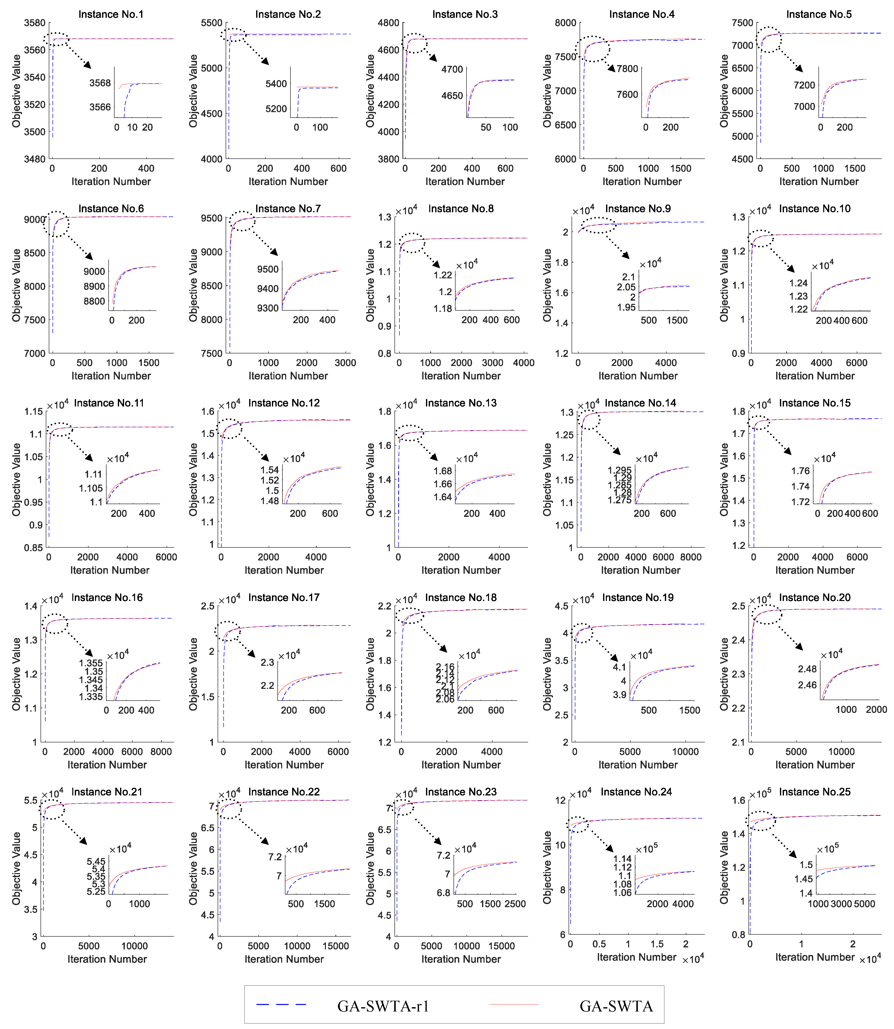
In order to verify the performance of the proposed initialization method, the random initialization method is used for comparison. Using the random initialization method means that the encoding of an individual is generated randomly without any prior knowledge. Since many of the evolutionary mechanisms used in ds-GA differ from the proposed algorithm, it is difficult to rule out the influence of different evolutionary mechanisms on algorithm performance. As a result, in order to ensure the fairness of the comparison, the proposed initialization method in GA-SWTA is replaced by the random initialization method. Meanwhile, the other mechanisms and parameters remain unchanged. The variant is called GA-SWTA-r1. We performed 30 independent runs on each algorithm for each instance. Figure 12 shows the results of the two algorithms.

From Figure 12, it can be found that the difference in the performance of the given indexes between GA-SWTA and GA-SWTA-r1 are very small. It means that the proposed initialization method does not affect the convergence of the algorithm. This is because the convergence of the proposed algorithm is mainly affected by the evolutionary operators. As the initialization method is designed to improve the quality of the initial population, its main function is to improve the efficiency of the convergence. In this paper, the evolution of the mean value of the objective value versus number of iterations is used to demonstrate the efficiency of the proposed initialization method. As we stop both of the algorithms until the best solutions found so far remain unchanged in 500 generations, the convergent generation of each run of the algorithm is different. Therefore, we calculate the maximum number of iterations of all the runs, then extend the number of iterations of all the runs to the same size as the maximum number. In this paper, the best objective value of each run is used as the value of the extended iteration. The results are shown in Figure 13.

As presented in Figure 13, the proposed initialization method can obtain a better initial value for almost all the instances. This means the proposed initialization method can generate a superior population at the beginning of the algorithm. In addition, for many instances, such as instances 2, 5, 9, 16, and 19, the maximum number of iterations of the proposed initialization method is remarkably less than the random method. This indicates our proposed method can effectively improve the convergence speed of the algorithm. Furthermore, for the very small-scale instances, instances No. 1 and No. 2, and the very large-scale instances, instances No. 21 to No. 25, our proposed initialization method is remarkably better than the random method. According to these experimental results, it can be concluded that the proposed initialization method can effectively improve the convergence efficiency of the algorithm, especially for the very small-scale and very large-scale S-WTA problems. This method cannot only improve the quality of the initial population, but also improve the convergence speed of the algorithm.

4.5. Experiments on Repair Operations

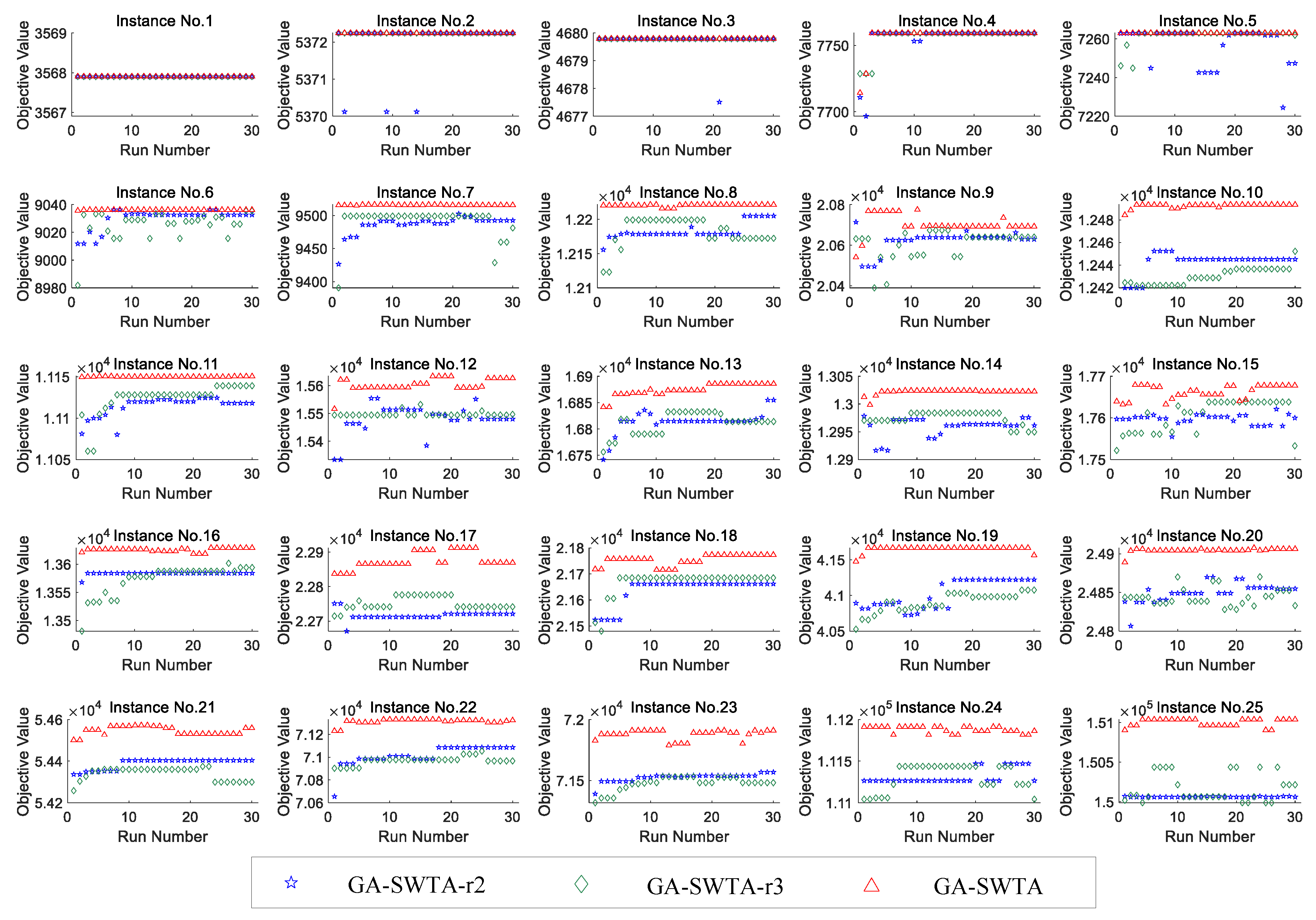
In this section, the performance of the repair operations is verified. In general, there are three methods to handle the individuals that do not satisfy the constraints. The first method is to delete the individuals. Although this method can quickly eliminate unsatisfactory individuals, it may reduce the efficiency of convergence. The second method is to punish the individuals. In this method, a penalty function is designed to adjust the objective values of the individuals, and the unsatisfactory individuals will be eliminated during the process of evolution. We should note that this method has been successful used in ds-GA to handling the constraints. The third method is to repair the individuals, which is used in our proposed algorithm. Therefore, the first and the second methods for handling constraints are selected for comparison.

Based on the proposed GA-SWTA, the repair operations are replaced by the first and the second methods. The variant is called GA-SWTA-r2, and GA-SWTA-r3, respectively. In GA-SWTA-r2, all unsatisfactory individuals are deleted instead of repair. In GA-SWTA-r3, the penalty function (7) is used to handling the constraints. Meanwhile, other mechanisms and parameters remain unchanged. We performed 30 independent runs on each algorithm for each instance. Figure 14 shows the results of the three algorithms.

As shown in Figure 14, GA-SWTA has the best performance on the given indexes for all the 25 instances. For the instance No. 1, all algorithms have the same performance. For the small-scale instances, No. 2 to No. 5, the performance of all the algorithms are very similar. In addition, for the majority of other instances, GA-SWTA-r2 has the worst performance. Based on analyzing the experimental results in Figure 14, we can conclude that the proposed repair method performs better than the other two methods in most of the instances. All the methods are work well on the small-scale problem. All these results show that the repair method proposed in this paper can effectively handle the constraints.

5. Conclusions

The STA and WTA problems have been widely concerned in the previous studies. However, few researches have focused on the S-WTA problem. In this paper, we proposed a novel genetic algorithm for the synthetical S-WTA problem. First, the frameworks of S-WTA are deeply analyzed. Then, a new model based on a novel framework of S-WTA is proposed. Furthermore, in order to solve the proposed model, a novel genetic algorithm, GA-SWTA, is presented. In the proposed GA-SWTA algorithm, a prior knowledge-based population initialization method is put forward to improve the efficiency of the convergence. Afterwards, two novel repair operations are designed to handle the constrains of the problem.

The performance of the GA-SWTA is analyzed in 25 test instances. Extensive experiments with two state-of-the-art heuristic algorithms and one GA-based algorithm demonstrate that our proposed algorithm outperforms other algorithms in most of the test instances. Furthermore, experiments on the proposed initialization method and random initialization method show that our proposed initialization method can improve the efficiency of the convergence. Moreover, the performance of the presented R-STA and R-WTA repair operations are detailed, which illustrate that these operations can effectively handle the constraints of the S-WTA problem as well as enhance the convergence of the algorithm.

According to these experimental results, we can conclude that our proposed algorithm can effectively solve the S-WTA problem. Compared with the traditional heuristic algorithms and evolutionary algorithm, the proposed algorithm has better convergence performance, which means that it can achieve better S-WTA scheme. However, since this algorithm is based on the framework of evolutionary computation, it cannot be performed in a real-time environment. Therefore, this proposed algorithm can be used in a non real-time and high-precision environment.

Although GA-SWTA can effectively solve the S-WTA problem in most of the test instances, its performance is worse than MRBCH in very large-scale problems. This is because the evolution operators used in this paper, which are the key factors to affect the convergence of GA-SWTA, are originally designed for the WTA problem, so they may lose their efficiency in solving S-WTA problems. Therefore, in our future work, we will focus on the design of evolution operators. We hypothesize that if the evolution operators are designed appropriately, the performance of the proposed algorithms in the very large-scale problems can be greatly enhanced.

In this paper, as we mainly focus on the framework of the S-WTA problem and the design of the solving algorithm, the configuration of the sensor–weapon system in practical application environment is neglected. Due to the rapid technological development of sensors like the array and wide range sensor systems, the sensor signal data can greatly affect the performance of the target detection and weapon guidance. In addition, the damage effect of the weapon on the target mainly depends on the type of targets and duration of destroying targets. Therefore, in our future work, we will also focus on these important elements, which may truly reflect the actual situation of the S-WTA problem, to build a more reasonable model.