Noise Reduction Mechanisms of an Airfoil with Trailing Edge Serrations at Low Mach Number

Abstract

Trailing-edge serrations have proven to be valid applications of trailing edge noise mitigation for an airfoil, while the physical noise reduction mechanism has not been adequately studied. We performed simulations employing Large-eddy simulation and the Lighthill–Curle method to reveal the variation in the hydrodynamic field and sound source due to the trailing edge serrations. The grid resolution and computational results were validated against experimental data. The simulation results show that: the trailing edge serrations impede the growth of spanwise vortices and promote the development of streamwise vortices near the trailing edge and the wake; the velocity fluctuations in the vertical cross-section of the streamwise direction near the trailing edge are reduced for the serrated airfoil, thereby obviously reducing the strength of the pressure fluctuations near the trailing edge; and the trailing edge serrations decrease the distribution of the sound source near the trailing edge and reduce the local peak value of sound pressure level in a specific frequency range as well as the overall sound pressure level. Moreover, we observed that, in the flow around the NACA0012 airfoil, the location where the strong sound source distribution begins to appear is in good agreement with the location where the separated boundary layer reattaches. It is therefore effective to reduce trailing edge noise by applying serrations on the upstream of the reattachment point.

1. Introduction

In recent years, with the development of civil aviation and the increasing popularity of air travel, the number of airports close to the city limits has grown rapidly. The persisting problem of aircraft noise in residential areas has attracted more and more attention and stringent standards have therefore been set by the International Civil Aviation Organization (ICAO) for aircraft noise control [1,2,3]. Noise generated from aircraft can be divided into two categories: engine noise and airframe noise. Engine jet noise used to be the major noise source for a civil aircraft, while, with the introduction of turbofan engines with high by-pass ratios, significant reductions of jet noise have been achieved. Therefore, nowadays, the reduction of the airfoil self-noise from the engine fan and airframe’s high lift devices has become more significant. Another industrial application in which the airfoil self-noise is also one of the dominant noise sources is the wind turbine. Wind turbines are an environmentally more acceptable form of energy, but noise nuisance, mainly radiated from the turbine blades, is created for communities living in close proximity [4]. Thus, for the aero-engine, airframe, and wind turbine industries, it is significant to reduce the airfoil self-noise [5,6].

Airfoil self-noise is created by the interaction of airflow with a wing or a blade. In particular, the interaction of the turbulent boundary layer with the airfoil trailing-edge is one of the dominant sources of airfoil self-noise [5]. For the aforementioned applications, the trailing edge noise is the most relevant noise source, especially at low Mach numbers since the turbulent fluctuations are scattered efficiently over a solid trailing edge [7]. For alleviating this dominant trailing edge noise, several passive noise-mitigation solutions such as trailing-edge brushes [8,9], sinusoidal and sawtooth serration [6,10,11,12,13,14,15,16], slits [17,18], and porous treatments [19,20,21] have been proposed. Among these passive methods, sinusoidal and sawtooth trailing edge serrations have been of important interest for researchers [3,6]. Many theoretical [22,23,24,25,26,27], experimental [10,15,16,28,29], and numerical [6,30,31] studies on trailing edge noise reduction using serrated trailing edges have been performed over the past decades.

The first theoretical model for a serrated trailing edge was developed by Howe [23,24] in 1991. Under the frozen turbulence assumption, an analytical noise radiation model was derived for the semi-infinite flat plate with both sinusoidal and sawtooth trailing edge serrations at low Mach number flow. According to Howe’s theory, since the effective spanwise length of the trailing edge that contributes to the trailing edge noise generation is reduced, trailing edge noise is consequently significantly reduced by the addition of trailing edge serrations. Howe’s theory states that, at high frequency, the reduction of trailing edge noise is about $10\times lo{g}_{10}(6h/\lambda )$ dB for the sinusoidal profile and is about $10\times lo{g}_{10}[1+{(4h/\lambda )}^2]$ dB for the sawtooth profile, where h and $\lambda$ are the amplitude and wavelength of the serrations, respectively. This theory is still widely used due to its simplicity. However, the predicted far-field noise spectra from this theory commonly deviate from experimental results [10,14,15,17,18,28,32]. Recently, Lyu et al. [26] proposed a more accurate semi-analytical model in which the predicted maximum noise reduction is better in agreement with measurements. However, some discrepancies concerning measurements are remaining due to the assumption of frozen turbulence [15,17]. Actually, from the limitations of the applicability of the analytical models, for further improvement of its accuracy, a characterization of the statistical properties of the surface pressure fluctuation on the serrations and their frequency and spatial dependence is indispensable [6].

Many experimental studies on trailing edge serrations have examined the disagreement between analytical predictions and experiments. Gruber [33] measured surface pressure fluctuations on serrations and showed that a larger spanwise magnitude-squared coherent of the surface pressure fluctuation on the straight trailing edge. Through incorporating surface pressure and surface heat transfer measurements, Chong and Vathylakis [14] showed the presence of pressure-driven edge-oriented vortices and concluded that the measured far-field noise is influenced by the angle between the edge-oriented vortices and the local streamline. Avallone et al. [15] showed the spanwise correlation length of the spanwise velocity component decreases from the root to the tip of serrations, while the convective velocity of the streamwise velocity component increases from the root to the tip and concluded that trailing edge noise is mainly generated at the root of the serrations. Based on the aforementioned experimental studies, it is possible to obtain further improvements with a better understanding of the effects of serrations on the wall pressure statistics. However, it has always been challenging for experimentalists to measure the surface pressure fluctuations on thin surfaces without perturbing the flow [14,33].

Computations of the flow organization and acoustic propagation around trailing edge serrations have been conducted in the past [6,11,30,31,34]. By performing numerical analyses, both flow and pressure fields can be obtained and one has the advantage of overcoming the experimental limitations mentioned above. Jones and Sandberg [11] found the formation of horse-shoe vortices in the space between the serrations. Avallone et al. [6] showed that the spanwise correlation length and convective velocity of surface pressure fluctuations influence both the intensity and the frequency range of noise reduction. Van der Velden [35] confirmed that the combed teeth give noise reductions larger than the standard teeth due to an improvement in the streamline angles: in general, the flow tends to be less three-dimensional and more aligned with the serration edge.

Although trailing edge serrations have proven to be valid solutions of trailing edge noise reduction, its underlying noise reduction mechanism is still not fully understood. A variation in the hydrodynamic field due to the spanwise varying geometry is a possible explanation. However, the complex three-dimensionality of the flow around the serrated trailing edges is not straightforward. An improvement in serration design can be realized with a better understanding of this underlying mechanism. Thus, the goal of this study was to show the variation in the hydrodynamic field caused by the trailing edge serrations and find the relation between the hydrodynamic field characteristics and noise-reduction. For this goal, the flow field around the NACA0012 airfoil with a straight trailing edge and sinusoidal serrated trailing edge at zero-angle of attack in low Mach number range were carefully investigated and compared. To overcome the experimental limitation, an efficient hybrid computational method for hydrodynamic field and aeroacoustic field was selected. The turbulent flows around NACA0012 airfoil with or without trailing edge serrations were computed through large-eddy simulation (LES) with an improved one-equation dynamic subgrid-scale (SGS) model. The weak compressibility at low Mach number was taken into account by modifying the pressure equation. The computational results were validated against experimental data. Acoustic perturbations were obtained utilizing a derived sound source formulation. This makes it possible to extend the hybrid method from zero to low or moderate Mach number region. A similar numerical methodology has been validated against experiments before, as presented in [36,37,38].

2. Computational Methodology

The following section describes the numerical methods used for determining the flow field though LES, accounting for the weak compressibility at low Mach number and noise source detection.

2.1. LES with One-Equation Subgrid Scale Model

The spatial filter operation and Favre-averaged filter are represented as $\overline{\left(\right)}$ and $\widetilde{\left(\right)}$ and applied to the governing equations. All variables are non-dimensioqnalized by chord length C and the mainstream velocity $U_0$. A general curvilinear coordinates ($\xi$, $\eta$, $\varsigma$) are used for all computations due to applying the boundary-fitted-grid. Thus, the governing equations can be written as [39]:

$$\frac{\partial \overline{\rho }}{\partial t}+\frac{1}{J}\frac{\partial }{\partial {\xi }^k}\left(J\overline{\rho }{\tilde{U}}^k\right)=0,$$

(1)

$$\frac{\partial \left(\overline{\rho }{\tilde{u}}_i\right)}{\partial t}+\frac{1}{J}\frac{\partial }{\partial {\xi }^k}\left(J\overline{\rho }{\tilde{u}}_i{\tilde{U}}^k\right)=-\frac{1}{J}\frac{\partial }{\partial {\xi }^k}\left[J\frac{\partial {\xi }^k}{\partial x_i}\left(\overline{p}+\frac{2}{3}\overline{\rho }{k}_{sgs}\right)\right]+\frac{1}{J}\frac{\partial }{\partial {\xi }^k}\left(J\frac{\partial {\xi }^k}{\partial x_i}{\sigma }_{ij}\right),$$

(2)

$$\overline{p}=\overline{\rho }RT,$$

(3)

where

$${\sigma }_{ij}=2\left(\frac{1}{Re}+\overline{\rho }{\nu }_{sgs}\right)\left({\tilde{S}}_{ij}-\frac{1}{3}{\delta }_{ij}{\tilde{S}}_{kk}\right),$$

(4)

$\rho$ represents the density, J is the Jacobian of the coordinate transformation, ${\overline{U}}^k$ is the contravariant velocity, $k_{sgs}$ is the subgrid scale kinetic energy, R is the ideal gas constant, T is the absolute temperature, ${\delta }_{ij}$ is the Kronecker symbol, $Re$ is the Reynolds number (as in $\rho U_{0}C/\nu$, where $\nu$ is molecular viscosity), ${\tilde{S}}_{ij}$ is the rate of strain tensor,

$${\tilde{S}}_{ij}=\frac{1}{2}\left(\frac{\partial {\xi }^k}{\partial x_i}\frac{\partial {\tilde{u}}_j}{\partial {\xi }^k}+\frac{\partial {\xi }^k}{\partial x_j}\frac{\partial {\tilde{u}}_i}{\partial {\xi }^k}\right),$$

(5)

and ${\nu }_{sgs}$ denotes the kinetic viscosity due to SGS turbulence that remains to be evaluated by a SGS model. Here, the SGS model is given in the following form:

$${\nu }_{sgs}=C_{\nu }{\Delta }_{\nu }\sqrt{k_{sgs}},$$

(6)

where $C_{sgs}$ is the model constant and ${\Delta }_{sgs}$ is the characteristic length given by Okamoto and Shina [40] in the following form

$${\Delta }_{\nu }=\frac{\overline{\Delta }}{1+C_k{\overline{\Delta }}^2{\left|\tilde{S}\right|}^2/k_{sgs}}.$$

(7)

Here, ${|\tilde{S}|}^2=\sqrt{2{\tilde{S}}_{ij}{\tilde{S}}_{ij}}$ denotes the norm of the rate-of-strain tensor, $C_k$ is the model constant and $\overline{\Delta }$ is the filter width. The transport equation of $k_{sgs}$ was theoretically derived by Yoshizawa and Horiuti [41] and then improved by Okamoto and Shima [40] and written as follows:

$$\begin{array}{ccc}\hfill \frac{\partial k_{sgs}}{\partial t}& +& \frac{1}{J}\frac{\partial }{\partial {\xi }^k}\left(J{k}_{sgs}{\tilde{U}}^k\right)=-{\tau }_{ij}{\tilde{S}}_{ij}-C_{\epsilon }\frac{k_{sgs}^{3/2}}{\Delta }\hfill \\ & -& 2\nu \left(\frac{\partial {\xi }^k}{\partial x_j}\frac{\partial \sqrt{k_{sgs}}}{\partial {\xi }^k}\right)\left(\frac{\partial {\xi }^l}{\partial x_j}\frac{\partial \sqrt{k_{sgs}}}{\partial {\xi }^l}\right)+\frac{1}{J}\frac{\partial }{\partial {\xi }^k}\left[\left(C_d{\Delta }_{sgs}\sqrt{k_{sgs}}+\nu \right){\gamma }^{kl}\frac{\partial k_{sgs}}{\partial {\xi }^l}\right],\hfill \end{array}$$

(8)

where $C_{\epsilon }$ and $C_d$ are model constants, ${\gamma }^{kl}$ is a symmetry tensor defined by

$${\gamma }^{kl}=J\frac{\partial {\xi }^k}{\partial x_m}\frac{\partial {\xi }^l}{\partial x_m},$$

(9)

and the production term $-{\tau }_{ij}{\tilde{S}}_{ij}$ is given as

$$-{\tau }_{ij}{\tilde{S}}_{ij}=\left[2{\nu }_{sgs}^{VM}\left({\tilde{S}}_{ij}-\frac{1}{3}{\delta }_{ij}-\frac{2}{3}{\delta }_{ij}{k}_{sgs}\right)\right]{\tilde{S}}_{ij}.$$

(10)

As a model of kinetic eddy viscosity ${\nu }_{sgs}^{VM}$, we introduce the Vreman model proposed by Vreman [42]:

$${\nu }_{sgs}^{VM}=C_{vm}\sqrt{\frac{B_{\beta }}{{\alpha }_{ij}{\alpha }_{ij}}},$$

(11)

where

$$B_{\beta }={\beta }_{11}{\beta }_{22}-{\beta }_{12}^2+{\beta }_{11}{\beta }_{33}-{\beta }_{13}^2+{\beta }_{22}{\beta }_{33}-{\beta }_{23}^2,$$

(12)

$${\beta }_{ij}={\Delta }_m^2{\alpha }_{mi}{\alpha }_{mj},{\alpha }_{ij}=\frac{\partial {\xi }^k}{\partial x_i}\frac{\partial {\tilde{u}}_j}{\partial {\xi }^k}.$$

(13)

Here, $C_{vm}(=0.025)$ is a constant model coefficient. The eddy viscosity is obtained from solving Equations (8) and (11) simultaneously. We call the new SGS eddy viscosity model as one-equation Vreman model.

2.2. Numerical Method for Weak Compressibility

Through introducing the concept of C-CUP method [43], the time marching of the compressible continuity and momentum equations is divided into two steps by the fractional step method and treated as the usual incompressible scheme. The time advancement approach of Equation (2) is divided as:

$$\frac{{\left(\overline{\rho }\tilde{\mathit{u}}\right)}^F-{\left(\overline{\rho }\tilde{\mathit{u}}\right)}^n}{\Delta t}=\nabla ·{[-\left(\overline{\rho }\tilde{\mathit{u}}\tilde{\mathit{u}}\right)+\tau ]}^n,$$

(14)

$$\frac{{\left(\overline{\rho }\tilde{\mathit{u}}\right)}^{n+1}-{\left(\overline{\rho }\tilde{\mathit{u}}\right)}^F}{\Delta t}=-\nabla {\overline{p}}^{n+1},$$

(15)

in which F represents the fraction step partially marched without the pressure gradient, n is the time step count, $\Delta t$ is the time increment and $\tau$ is the viscous stress. The time marching method of Equation (1) is given as:

$$\frac{{\overline{\rho }}^{n+1}-{\overline{\rho }}^n}{\Delta t}+\nabla ·{\left(\overline{\rho }\tilde{\mathit{u}}\right)}^{n+1}=0.$$

(16)

Taking the divergence of Equation (15) and substituting that into Equation (16) derives the elliptic equation for ${\overline{p}}^{n+1}$:

$$\frac{1}{\Delta t}\left[-\frac{{\overline{\rho }}^{n+1}-{\overline{\rho }}^n}{\Delta t}-\nabla ·{\left(\overline{\rho }\tilde{\mathit{u}}\right)}^F\right]=-{\nabla }^2{\overline{p}}^{n+1}.$$

(17)

To account for the compressibility for the pressure equation, assuming that flow field is isothermal and the change of $\Delta \overline{p}$ and $\Delta \overline{\rho }$ is small in $\Delta t$, Equation (3) can be written as

$${\overline{p}}^{n+1}-{\overline{p}}^n=({\overline{\rho }}^{n+1}-{\overline{\rho }}^n)RT.$$

(18)

Substitution of Equation (18) into Equation (17) leads to a pressure equation considering the compressibility given as follows:

$${\nabla }^2{\overline{p}}^{n+1}-\frac{{\overline{p}}^{n+1}}{{(\Delta t)}^{2}RT}=\frac{\nabla ·{\left(\overline{\rho }\tilde{\mathit{u}}\right)}^F}{\Delta t}-\frac{{\overline{p}}^n}{{(\Delta t)}^{2}RT}.$$

(19)

Thus, the compressibility effect is represented by the second term of both sides of Equation (19). In short, ${\overline{p}}^{n+1}$ is calculated by Equation (19) and then ${\left(\overline{\rho }\tilde{\mathit{u}}\right)}^{n+1}$ is obtained from Equation (14), and finally ${\overline{\rho }}^{n+1}$ is solved by Equation (1). As mentioned above, our method is suitable for treating the density variation in low Mach number flows without using any artificial compressibility parameters since the assumption of small change of $\Delta \overline{p}$ and $\Delta \overline{\rho }$ is valid in low Mach number flows, rather than in a high Mach number flow.

2.3. Acoustic Equations

The compressible continuity equation and Navier–Stokes equation are given as:

$$\frac{\partial \rho }{\partial t}+\frac{\partial \left(\rho u_j\right)}{\partial x_j}=0,$$

(20)

$$\frac{\partial \left(\rho u_i\right)}{\partial t}+\frac{\partial }{\partial x_j}\left(\rho u_i{u}_j\right)+\frac{\partial p}{\partial x_i}=\frac{\partial {\sigma }_{ij}}{\partial x_j},$$

(21)

where

$${\sigma }_{ij}=2\mu \left(S_{ij}-\frac{1}{3}{\delta }_{ij}{S}_{ij}\right),S_{ij}=\frac{1}{2}\left(\frac{\partial u_i}{\partial x_j}+\frac{\partial u_j}{\partial x_i}\right).$$

(22)

The density and pressure of flow field can be decomposed as the mean component and perturbation component:

$$\rho ={\rho }_0+{\rho }^{\prime },p=p_0+p^{\prime }$$

(23)

where due to low Mach number

$${\rho }_0\gg {\rho }^{\prime },p_0\gg p^{\prime }.$$

(24)

By multiplying $u_i$ by Equation (20) and ${\rho }^{\prime }$ by Equation (21), taking the divergence of the sum, subtracting time derivation of the mass conservation law in Equation (20) and adding $-c_0^2\frac{{\partial }^2\rho }{\partial x_i\partial x_i}$ with respect to the equation both sides, we finally obtain an approximation wave equation with the velocity divergence as the sound source:

$$\frac{{\partial }^2\rho }{\partial t^2}-c_0^2\frac{{\partial }^2\rho }{\partial x_i\partial x_i}={\rho }_0\nabla ·\left[(\mathit{u}·\nabla )\mathit{u}\right].$$

(25)

Our wave equation (Equation (25)) with the velocity divergence ${\rho }_0\nabla ·\left[(\mathit{u}·\nabla )\mathit{u}\right]$ as the sound source is similar to Powell’s wave equation [44] with the vorticity ${\rho }_0\nabla ·(\mathit{\omega }\times \mathit{u})$ as the sound source. Obviously, two wave equations both take the effect of the compressibility into account.

Applying ${\rho }_0\nabla ·\left[(\mathit{u}·\nabla )\mathit{u}\right]$ in Equation (25) as sound source to predict sound field, the sound pressure in the far field can be obtained by solving Equation (25) using the compact Green’s function [45]. Assuming that the object is stationary, the velocity at the boundary S of the object is 0, and the observation point x is sufficiently far from the sound source area y, Equation (25) can be expanded as follows by using Green’s formula:

$$p_a(\mathit{x},t)=-{\rho }_0\int \int \left[(\mathit{u}·\nabla )\mathit{u}\right]·\nabla G(\mathit{x},\mathit{y},t-\mathit{\tau })d^3\mathit{y}d\mathit{\tau },$$

(26)

where $p_a$ means pressure sound and G is the compact Green function, which can be expressed as

$$G(\mathit{x},\mathit{y},t-\mathit{\tau })=\frac{1}{4\pi \left|\mathit{x}\right|}\delta \left(t-\mathit{\tau }\frac{\left|\mathit{x}\right|}{c_0}\right)+\frac{\mathit{x}·\mathit{Y}}{4\pi c_0{\left|\mathit{x}\right|}^2}\frac{\partial }{\partial t}\delta \left(t-\mathit{\tau }-\frac{\left|\mathit{x}\right|}{c_0}\right).$$

(27)

Here, $\mathit{Y}$ is Kirchhoff vector and can be solved by ${\nabla }^2{\mathit{Y}}_i=0$. Substituting Equation (27) into Equation (26) leads to

$$p_a(\mathit{x},t)=-\frac{{\rho }_0{x}_i}{4\pi c_0{\left|\mathit{x}\right|}^2}\frac{\partial }{\partial t}\int \left[(\mathit{u}·\nabla )\mathit{u}\right]\left(\mathit{y},t-\frac{\left|\mathit{x}\right|}{c_0}\right)\nabla {\mathit{Y}}_i\left(\mathit{y}\right)d^3\mathit{y}.$$

(28)

From Equation (28), Fourier transform is performed to obtain $p_a^{\prime }$. Using the obtained $p_a^{\prime }$, the sound pressure level (SPL) is determined by the following equation:

$$SPL\left(dB\right)=10\times log\left(\frac{{p_a^{\prime }}^2}{P_b^2}\right),$$

(29)

where $P_b$ represents the reference pressure, and its magnitude is $P_b=2\times {10}^{-5} \mathrm{Pa}$.

3. Computational Setup and Test Case

The object of calculation was the three-dimensional flow around baseline NACA0012 airfoil and the NACA0012 airfoil with the trailing edge serrations. The schematics of the serrated airfoils from top view, center cross section and side cross section are shown in Figure 1. The serration wavelengths and the serration depths were $\lambda /C=0.2$ and $h/C=0.1$, respectively. The airfoil thickness was changed starting at 80% the chord length from the leading edge.

The computational domain and boundary conditions for NACA0012 airfoil and serrated airfoils are shown in Figure 2. A Cartesian coordinate system was used to define x in the mainstream direction, z in spanwise direction and y in the vertical direction (perpendicular to x and y). The boundary-fitted grid of C-type was applied in the $x-y$ plane. Actually, all computations were conducted on a general curvilinear coordinate system ($\xi$, $\eta$, $\zeta$), in which $\xi$ means the direction following the mainstream surface of the airfoil, $\eta$ is the direction away from the surface of airfoil, and $\zeta$ is the same as the direction of z. The computational domain size was defined as follows: the diameter of a half-circle of C-type grid is $8C$; and the length of the wake side and the spanwise side are $8C$ and $0.5C$, respectively, where C is chord length. As shown in Figure 2, the inflow was a uniform stream without disturbance. Thus, the turbulence was developed in the boundary layer around the airfoil after the transition. The outflow boundary condition was defined as the convective boundary condition. In the spanwise direction, the periodic boundary condition was used. The gradients of variables in the $\zeta$ direction at the top and bottom boundary were assumed to be zero. The nonslip boundary condition was applied at the surface of the airfoil. To remove the reflection of pressure waves, for pressure, a non-reflective boundary condition by Okita and Kajishima [46] was used in the boundary condition of inflow, outflow, top, and bottom.

A second-order central finite-difference discretization scheme was used for the diffusion terms in the equation of motion, and the QUICK method for the convective terms. The QUICK method used here is to reduce the numerical instability resulting from the grid arrangement based on the general curvilinear coordinate system in high Reynolds number flow. As shown in Section 2.2, the fractional method was selected for coupling the continuity equation and the pressure field. For the time advancement, the second-order accuracy Adams–Bashforth method was used for the convective term and viscous term in the Navier–Stokes equation. For the transport equation of the SGS kinetic energy, the donor cell method was employed as spatial discretization scheme, and the second-order accuracy Adams–Bashforth method was utilized to the convective, production, dissipation and diffusive terms. The initialization data of $K_{sgs}$ was solved from $k_{sgs}={\left({\nu }_{sgs}/C_{\nu }\overline{\Delta }\right)}^2$ using the results of ${\nu }_{sgs}$ from LES with Vreman model.

Computational parameters of all possible cases conducted in this study are summarized in

Table 1. Computational parameters.

Case	$\mathit{Ma}(\times {10}^{-2})$	$\mathit{Re}(\times {10}^5)$	Angle of Attack	${\mathit{N}}_{\mathit{x}}\times {\mathit{N}}_{\mathit{y}}\times {\mathit{N}}_{\mathit{z}}$	${\Delta }_{\mathit{x}}^{+},{\Delta }_{\mathit{y}}^{+},{\Delta }_{\mathit{z}}^{+}$
Straight-1	$8.75$	2	$9^{\circ }$	$1600\times 160\times 60$	$40,1.2,40$
Straight-2	$8.75$	2	$9^{\circ }$	$1600\times 160\times 20$	$40,1.2,80$
Straight-3	$8.75$	2	$9^{\circ }$	$1600\times 160\times 100$	$40,1.2,24$
Straight-4	1	2	$9^{\circ }$	$1600\times 160\times 60$	$40,1.2,40$
Straight-5	0	2	$9^{\circ }$	$1600\times 160\times 60$	$40,1.2,40$
Straight-6	$8.75$	2	$0^{\circ }$	$1600\times 160\times 60$	$40,1.2,40$
Serrated-1	$8.75$	2	$0^{\circ }$	$1600\times 160\times 60$	$40,1.2,40$

. First, straight and serrated in the first column of Table 1 mean the NACA 0012 airfoil with straight trailing edge and serrated trailing edge. To validate numerical method of this study, we conducted LES of the compressible flow around NACA0012 airfoil with the angle of attack, $9^{\circ }$; the Reynolds number based on the chord length and the mainstream velocity, $2\times {10}^5$; and the Mach number, $8.75\times {10}^{-2}$, which matches the computational setup of Kato et al. [47] and the experimental setup of Miyazawa et al. [48]. To exclude the effect of Mach number on the numerical method, we performed simulations of Mach numbers 0, $0.01$ and $0.0875$ under the same Reynolds numbers, angle of attack and mesh arrangement. To investigate the dependence of the grid resolution, we changed the resolution in the spanwise direction to 20, 60 and 100 under the same other conditions of the first calculation. To elucidate the relationship between the variation in the hydrodynamic field due to trailing edge serrations and the underlying noise reduction mechanism, NACA0012 airfoil with serrated and straight trailing edges at zero angle of attack was computed. The condition of $0^{\circ }$ angle of attack was selected since the effect of the serration loading on the hydrodynamic flow and the radiated noise can be isolated. In Table 1, $N_{\alpha }$ and ${\Delta }_{\alpha }^{+}$ denote the number of grid points and grid spacing in the $\alpha$ direction. The superscript + means the wall unit, that is,

$${\Delta }_{\alpha }^{+}=\frac{u_{\tau {\Delta }_{\alpha }}}{\nu },u_{\tau }=\sqrt{\frac{{\tau }_w}{\rho }},$$

(30)

where $u_{\tau }$ is the averaged local wall friction velocity and ${\tau }_w$ denotes the wall stress. In Table 1, the grid width in wall unit was obtained on the suction side at $X/C=0.5$.

4. Grid Resolution Study and Validation of Numerical Method

Hereafter, the data were collected by time-averaging and spatial averaging in the spanwise direction. Before discussing the results of the numerical investigation, we first examine the dependence of the intensity of fluctuation of the pressure coefficient on the grid resolution, as shown in Figure 3. Here, the pressure coefficient $C_p$ is defined using the freestream pressure $p_0$, that is, $C_p=(p-p_0)/\frac{1}{2}\rho U_0^2$. Then, $C_{prms}$ means the root-mean-square of $C_p$. Since the resolution in the spanwise direction most affects the turbulence statistics, the grid points in the spanwise direction were set as $N_z=20,60,100$ for a fixed spanwise direction length, as shown Straight-1, -2, and -3 cases in Table 1. In Figure 3, when the grid resolution in the spanwise direction is low, i.e., $N_z=20$, the peak value of $C_{prms}$ is overestimated compared to the other cases. However, in the case of $N_z=60$ and more grid points $N_z=100$, there is almost no difference in the peak value of $C_{prms}$. Therefore, it was shown that the peak value of $C_{prms}$ does not depend on the grid resolution if the grid resolution that can reproduce the anisotropy of the wall turbulence properly is ensured.

To demonstrate the validity of the numerical method, we compared the results of the present numerical model with the experimental and computational data obtained by Miyazawa et al. [48] and Kato et al. [47], respectively. As for $C_p$ in Figure 4, the results of our model and the experimental data are in good agreement. There is almost no difference in the distribution of $C_p$ on the airfoil due to the change in the Mach number. Comparing the results of the present model at Mach number $M=0$ with the results of Kato et al., overall good agreement can be seen apart from differences near the leading edge of the airfoil. This difference is believed to be due to the difference of the SGS model. With regard to $C_{prms}$ on the suction surface side of the airfoil in Figure 5, the location of the peak value of $C_{prms}$ agrees well with the experimental data regardless of the Mach number, but there is a big difference in the peak value corresponding to the change of Mach number. In the case of $M=0.0875$, which is the same setup as in the experiment, the agreement of the profile of $C_{prms}$ between the simulation and experiment is quite good at all locations. In the case of $M=0$, the profile of $C_{prms}$ agrees well with the experimental data from the airfoil center to the trailing edge, while the peak value of $C_{prms}$ near the leading edge is overestimated compared to the experimental data. The results of Kato et al. show the same tendency as that of $M=0$, although they adopted a different SGS model for a different case. Thus, we believe that the overestimation of $C_{prms}$ observed near the leading edge in the cases of $M=0$ and Kato et al. is caused by not considering the effect of compressibility near the leading edge of the airfoil. These observations therefore mean that the effect of compressibility cannot be ignored in the vicinity of an airfoil even under low Mach number conditions and the present numerical method is suitable for considering the weak compressibility at low Mach number and then in reasonable agreement with the experimental data.

5. Effect of Serrations on the Hydrodynamic Field

In this section, the results of flow fields around baseline NACA0012 airfoil and that with sinusoidal trailing edge serrations at zero angle of attack, Mach number $M=0.0875$, Reynolds number based on the chord length and the mainstream velocity $Re=2\times {10}^5$ are compared to discuss the effect of serrations on the hydrodynamic field and then to understand the underlying noise reduction mechanism of trailing edge serrations. Figure 6 shows the mean velocity distribution in the main flow direction around the straight and serrated NACA0012 airfoils, i.e., around the baseline NACA0012 airfoil in Figure 6a and around the cross-section $A^{\prime }A$, and $B^{\prime }B$ of the serrated airfoil in Figure 6b. In Figure 6a, the separation appears near the trailing edge and the region of separation is small. However, in the case of an airfoil with trailing edge serrations shown in Figure 6b, a wide separation area is seen near the root of the serration (cross-section $A^{\prime }A$) compared to the average velocity distribution around the straight airfoil. The expansion of the separation area near the trailing edge delays the pressure recovery and leads to an increase in pressure drag on the serrated airfoil. As a result, the drag coefficient of the serrated airfoil is larger than that of the baseline NACA0012 airfoil, that is, $C_D=1.27\times {10}^{-2}$ and $1.13\times {10}^{-2}$ for the serrated and straight airfoils, respectively. It is therefore confirmed that the pressure drag is slightly increased by the trailing edge serration.

To investigate the variation of the vortex structure due to the trailing edge serration, the iso-surface of the second invariant $Q=400$ of the instantaneous velocity gradient tensor is shown in Figure 7. The value of the mainstream direction vorticity ${\omega }_x$ is expressed in color gradation on the Q iso-surface, where the red corresponds to ${\omega }_x=100$ and blue corresponds to ${\omega }_x=-100$. In the case of the flow around the NACA0012 airfoil in Figure 7a, spanwise vortices with a numerical value of $Q=400$ or more are observed from around $X/C=0.82$, and it is confirmed that these vortices are three-dimensionalized and collapse into small vortices while advancing downstream along the airfoil surface. Finally, vortices structures with large values of ${\omega }_x$ in the near wake are hardly found. In the case of the flow around the trailing edge serration in Figure 7b, by contrast, almost no spanwise vortices with a value of $Q=400$ or more can be seen near $X/C=0.82$, and the vortices structure with finer space scales including mainstream and spanwise vortices is generated near the trailing edge. Meanwhile, it is observed that large vortex structures including strong streamwise direction vortexes are developed in the near wake.

For the sake of investigating the behavior of the vortices near the trailing edge serrations in more detail, Figure 8 shows the time evolution of the instantaneous vortical structure ($Q=2000$ iso-surface) colored by $|{\omega }_x|\le 100$ near the trailing edge of the serrated airfoil (time interval is about $1.5\times {10}^{-3}$ s). Focusing on the red-lined vortices in Figure 8a, the three dimensional small vortices seen near the root of serration are stretched as they move downstream in the near tip of the serration, as shown in Figure 8b, and then they become larger-scale mainstream direction vortices in the near wake in Figure 8c. From the above observations, it is confirmed that the growth of the spanwise vortices near the trailing edge is impeded by the trailing edge serration, and the main flow direction vortex is formed and developed from near the trailing edge to the wake for the flow field around the serrated airfoil. Consequently, the development of these mainstream vortices will greatly affect the fluctuation components in the vertical cross section of the mainstream direction.

Figure 9 and Figure 10 show the distributions of Reynolds stress $R_{ij}$ near the trailing edge of the flow around the NACA0012 airfoil and around the trailing edge serrated NACA0012 airfoil. Reynolds stress is defined by $R_{ij}=\tilde{\rho }\overline{u_i^{\prime }{u}_j^{\prime }}$. Figure 9 shows an iso-surface of $R_{22}=0.05$, and Figure 10 shows an iso-surface of $R_{33}=0.02$. In the case of the flow field around the baseline NACA0012 blade, $R_{22}$ is distributed in the spanwise direction on the airfoil surface near the trailing edge and near the wake, while, in the case of the trailing edge serrated airfoil, the distribution of $R_{22}$ is almost limited near the wake. Meanwhile, $R_{33}$ is widely distributed near the wake of the serrated airfoil, while it is hardly found near the wake of the baseline airfoil. From this, it is found that the development of the vortices in the main flow direction due to the trailing edge serrations of airfoil results in a decrease in velocity fluctuations in the vertical cross-section of the mainstream direction.

Figure 11 shows the pressure fluctuation distribution of the airfoil surface near the trailing edge of baseline NACA0012 airfoil and that with the trailing edge serrations. In the case of the NACA0012 airfoil shown in Figure 11a, a strong pressure fluctuation distribution is observed across the entire spanwise direction near the trailing edge, while, in the case of the serrated airfoil shown in Figure 11b, the pressure fluctuation is weaker and mainly concentrated at the tips of the serrations. The profiles of pressure fluctuation near the trailing edge of the baseline NACA0012 airfoil and the serrated airfoil are similar to the distribution of Reynolds stress in Figure 9. It is therefore believed that the distribution of Reynolds stresses affects the strength of the pressure fluctuation.

From the above discussion, although the trailing edge serrations cause an increase in pressure drag on the airfoil, they prevent the growth of spanwise vortices near the trailing edge and promote the development of the streamwise direction vortices. Meanwhile, the velocity fluctuation in the vertical cross-section of the mainstream direction is mitigated due to the trailing edge serrations, and, as a result, brings a decrease in the pressure fluctuation near the trailing edge.

6. Effect of Serrations on the Sound Field

Figure 12 shows the distribution of sound source ${\rho }_0\nabla ·\left[(\mathit{u}·\nabla )\mathit{u}\right]$ around the baseline NACA0012 airfoil and the trailing edge serrated airfoil. The value of ${\rho }_0\nabla ·\left[(\mathit{u}·\nabla )\mathit{u}\right]$ is slightly smaller near the trailing edge in the case of the serrated airfoil (section $B^{\prime }B$) than that in the case of the baseline NACA0012 airfoil. At the root of the serrations (section $A^{\prime }A$), a relatively strong distribution of ${\rho }_0\nabla ·\left[(\mathit{u}·\nabla )\mathit{u}\right]$ is confirmed in comparison with that at the section $B^{\prime }B$, while in the wake away from the trailing edge of $A^{\prime }A$ there is no strong distribution of sound source compared to in the wake of section $B^{\prime }B$. This is believed to be due to the reduction of fluctuation components in the vertical cross-section of the mainstream direction, which is thought to be due to the development of a strong main flow direction vortex near the wake of section $A^{\prime }A$ compared to near the wake of section $B^{\prime }B$ in Figure 9 and Figure 10. 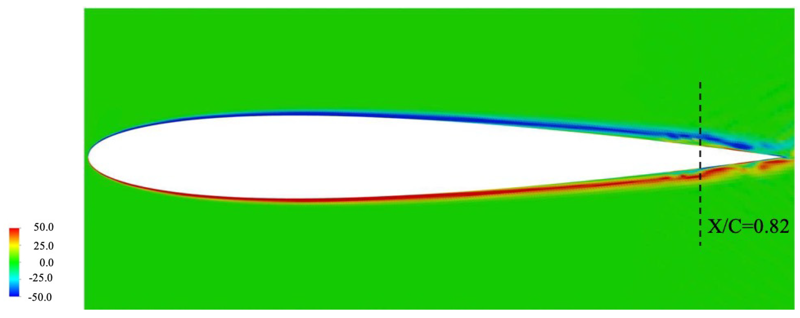Figure 13 and Figure 14 show the instantaneous distribution of the spanwise direction vorticity ${\omega }_z$ around the baseline airfoil and the profile of averaged friction coefficient on the suction side of NACA0012 airfoil, respectively. In Figure 12a, it is shown that the strong sound source near the trailing edge is distributed at the location of $x/C=0.82$, which can be confirmed by the distribution of the spanwise direction vorticity ${\omega }_z$ (see Figure 13). It is interesting that the strong sound source location of $x/C=0.82$ is in good agreement with the position where the separated boundary layer reattaches at the trailing edge of the airfoil (see Figure 14). From this observation, it can be said that it is effective to reduce the strong sound source around an airfoil due to the reattachment of the separated boundary layer by using serration before reattaching the separated boundary layer.

The sound source, as shown in Figure 12, was used to calculate the sound pressure. Figure 15 compares the sound pressure level (SPL) measured at a point $0.5$ m from the trailing edge in the direction normal to the mainstream velocity for the $x-y$ plane. The SPL obtained by the Lighthill–Curle method [45] using our LES database is compared. In addition, the experiment results by Hayashi et al. [49] measured at same condition are also shown for comparison. In Figure 15, the SPL profile obtained from the flow field around the baseline NACA0012 airfoil is in reasonable agreement with the experimental data between 1000 and 3000 Hz. Especially, the location of the peak SPL around 1800 Hz seen in the experimental data are well reproduced, while the value of the peak SPL seen in the measurement is slightly underestimated. For the SPL profile obtained from the flow field around the serrated airfoil, the peak value near 1800 Hz disappears and the peak value is seen around 2000 Hz. However, it can be seen that the peak value for the serrated airfoil is smaller than the value for the baseline airfoil, specifically 83 dB for the peak value of baseline airfoil and 91 dB for the peak value of serrated airfoil. On the other hand, the overall sound pressure level (OASPL) obtained by summing up for each frequency band is determined by the following equation:

$$\mathrm{OASPL}\left(\mathrm{dB}\right)=10\times log\left[\int (\frac{p_a^2}{p_b^2})df\right],$$

(31)

where f means frequency. The OASPL of the baseline airfoil is compared with that of the serrated airfoil, resulting in a reduced OASPL for the serrated airfoil. More specifically, in the frequency band range from 146 to 10,000 Hz, the OASPL of the baseline NACA0012 and serrated airfoils are 81 dB and 73 dB, respectively. Thus, the airfoil with trailing edge serrations indicates that both the local peak SPL near 1800 Hz and the overall SPL are reduced.

From the above observations, it is shown that the airfoil with trailing edge serrations decreases the distribution of the sound source near the trailing edge and also reduces the overall SPL as well as the local peak value of SPL in a specific frequency range. In particular, in the flow around NACA0012 airfoil, the location where the strong sound source distribution begins to appear and the location where the separated boundary layer reattaches is in good agreement. Therefore, it can be said that applying serrations on upstream of the reattachment point for an airfoil is effective in terms of noise reduction.

7. Conclusions

The turbulent flow over a NACA0012 airfoil with a straight trailing edge and serrated trailing edge at zero-angle of attack in low Mach number range and the resulting sound field and trailing edge noise were studied to investigate the underlying noise reduction mechanism. Especially, a variation in the hydrodynamic field due to the varying geometry at trailing edge was studied. The flow field was computed by LES with an improved one-equation dynamic SGS model. The weak compressibility at low Mach number was taken into account by modifying the pressure equation. The acoustic far-field was obtained by means of the Lighthill–Curle method [45]. A grid resolution study and comparison against experimental data was used to assess the computational set-up. The computational results were validated against experimental data [47,48]. It was confirmed that the serrated airfoil reduces the trailing edge noise, while the flow around a serrated airfoil shows an expansion of the separation area near the trailing edge, resulting in slightly increasing pressure drag. It was found that the trailing edge serrations of an airfoil impede the growth of the spanwise vortices near the trailing edge and promote the development of the streamwise vortices near the trailing edge and the wake. Meanwhile, the velocity fluctuations in the vertical cross-section of the mainstream direction near the trailing edge are reduced by the serrated airfoil in comparison with the baseline NACA0012 airfoil. As a result, the strength of the pressure fluctuation is reduced near the trailing edge. Especially, in the flow around the baseline airfoil, the location where the strong sound source distribution begins to appear is in good agreement with the location where the separated boundary layer reattaches. Thus, application of the trailing edge serrations on the upstream of the reattachment point for an airfoil is effective to reduce the strong sound source and then consequently is effective for noise reduction.