Spatial Prediction of Landslide Susceptibility Using GIS-Based Data Mining Techniques of ANFIS with Whale Optimization Algorithm (WOA) and Grey Wolf Optimizer (GWO)


 ,
,  ,
,  ,
,  ,
,  , , , ,
  ,
,  ,
,
Abstract
1. Introduction
2. Material and Methods
2.1. Introduction of the Study Area
2.2. Data Preparation
2.2.1. Landslide Inventory Map
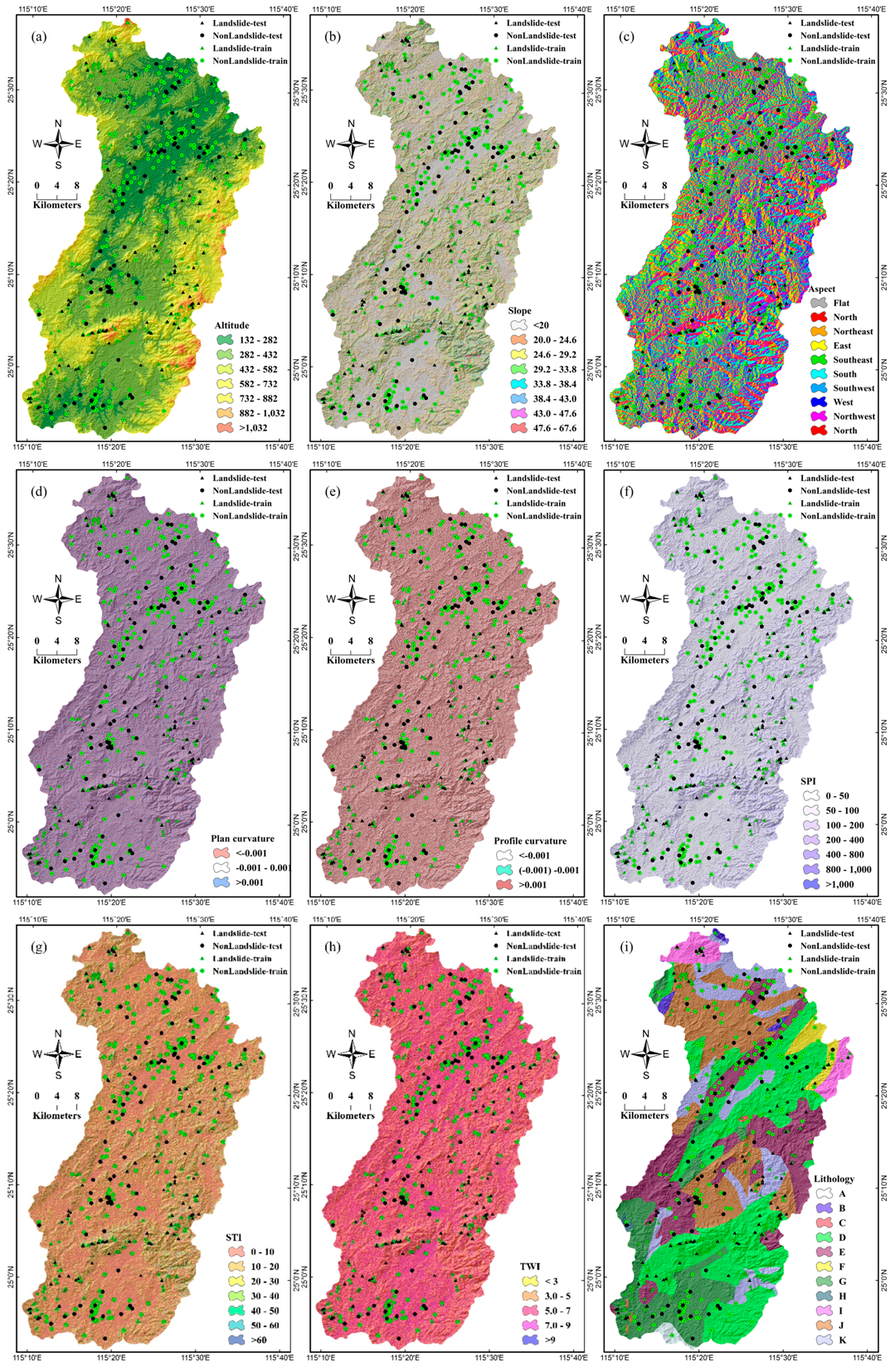
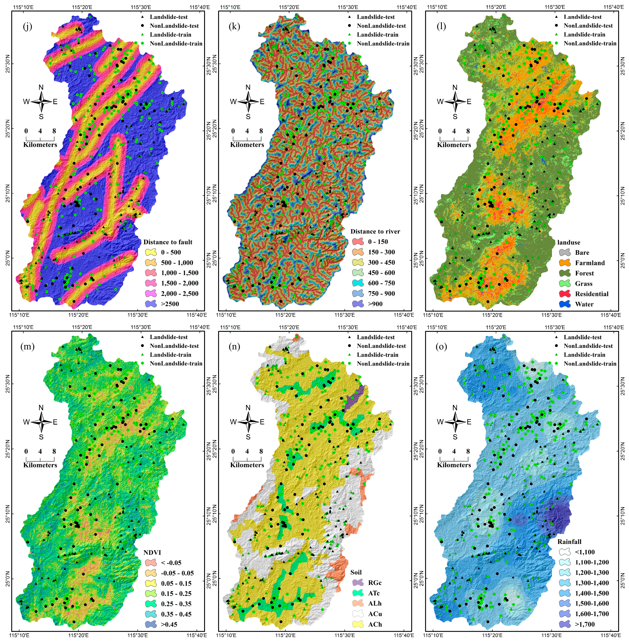
2.2.2. Landslide Influencing Factors
2.3. The Initial Weights for Modelling Process
2.4. Landslide Prediction Models
2.4.1. ANFIS
- Rule 1: If x1 and x2 are A1 and B1, respectively, then f1 = p1x1 + q1x2 + r1.
- Rule 2: If x2 and x2 are A2 and B2, respectively, then f2 = p2x2 + q2x2 + r2.
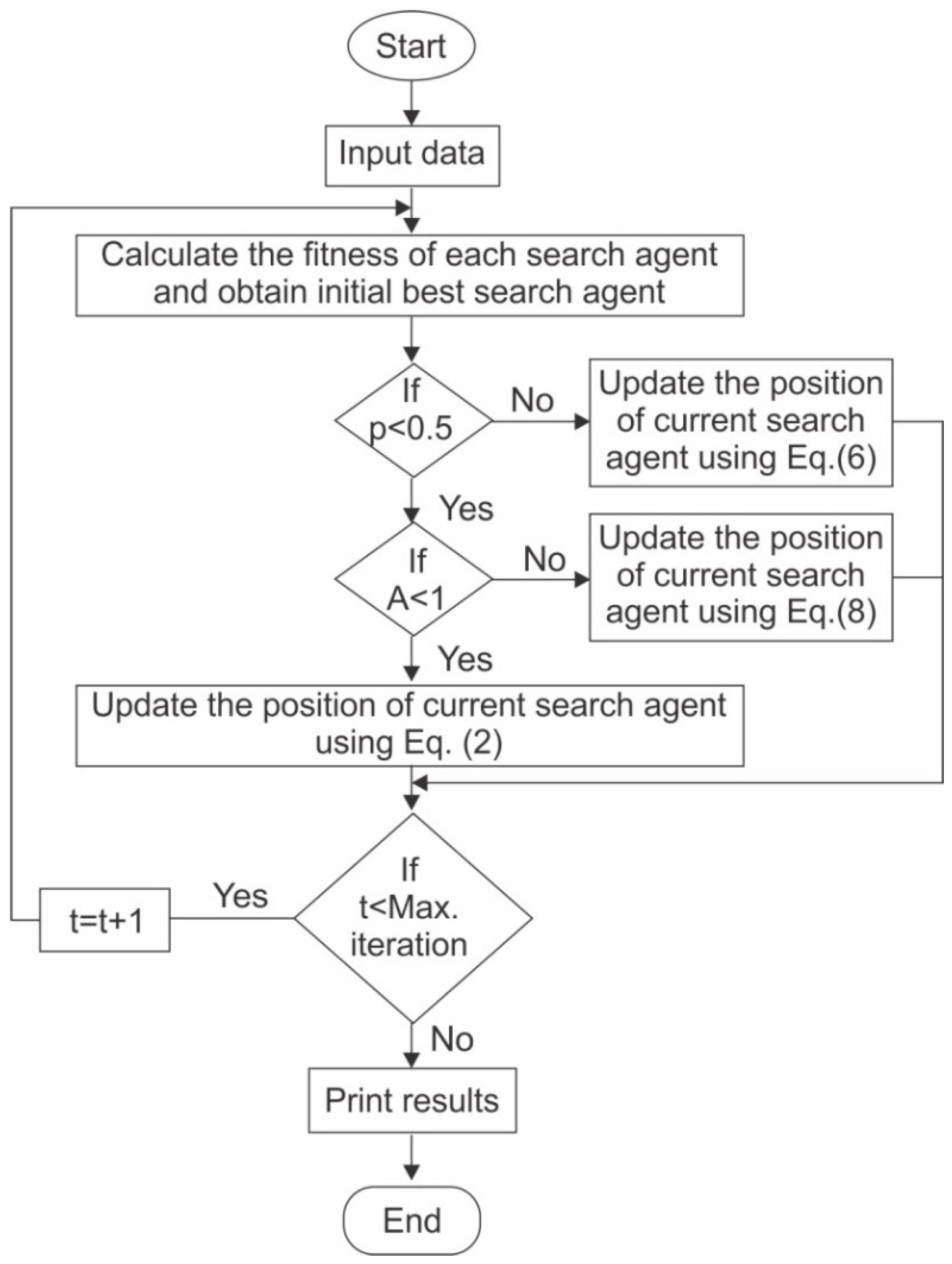
2.4.2. Whale Optimization Algorithm (WOA)
2.4.3. Grey Wolf Optimizer (GWO)
2.4.4. Particle Swarm Optimization (PSO)
3. Results and Validation
3.1. Correlation between Landslides and Influencing Factors Based on SWARA
3.2. Application of the Integrated ANFIS Methods
3.3. Preparation of Landslide Susceptibility Mapping
3.4. Validation of the Resultant Maps
4. Discussion
5. Conclusions
- (1)
- SWARA-ANFIS-GWO has the best result in terms of the convergence of objective function in comparison to SWARA-ANFIS-WOA.
- (2)
- SWARA-ANFIS-GWO outperforms SWARA-ANFIS-WOA and thus is a better tool for landslide susceptibility modelling.
- (3)
- The hybrid SWARA-ANFIS-GWO method has better goodness-of-fit and prediction accuracy and can produce more accurate reliable results. Therefore, it is recommended for LSM in other dangerous areas.
- (4)
- In the study area, the landslides are prone to occur under conditions of slop with >47.6°, south aspect, altitude with 882–1032 m, plan curvature with >0.001, profile curvature with <−0.001, SPI with 800–1000, TWI with 3–5, lithology of Lu jing Unit, distance to fault with 0–500 m, distance to river with 600–750 m, forest land-uses, NDVI with 0.35–0.45, soil of ACu and 1500–1600 mm rainfall.
Author Contributions
Funding
Conflicts of Interest
References
- Bovenga, F.; Pasquariello, G.; Pellicani, R.; Refice, A.; Spilotro, G. Landslide monitoring for risk mitigation by using corner reflector and satellite sar interferometry: The large landslide of Carlantino (Italy). Catena 2017, 151, 49–62. [Google Scholar] [CrossRef]
- Torizin, J.; Fuchs, M.; Awan, A.A.; Ahmad, I.; Akhtar, S.S.; Sadiq, S.; Razzak, A.; Weggenmann, D.; Fawad, F.; Khalid, N. Statistical landslide susceptibility assessment of the mansehra and torghar districts, khyber pakhtunkhwa province, pakistan. Nat. Hazards 2017, 89, 757–784. [Google Scholar] [CrossRef]
- Di Martire, D.; Paci, M.; Confuorto, P.; Costabile, S.; Guastaferro, F.; Verta, A.; Calcaterra, D. A nation-wide system for landslide mapping and risk management in italy: The second not-ordinary plan of environmental remote sensing. Int. J. Appl. Earth Obs. Geoinf. 2017, 63, 143–157. [Google Scholar] [CrossRef]
- Crozier, M. A proposed cell model for multiple-occurrence regional landslide events: Implications for landslide susceptibility mapping. Geomorphology 2017, 295, 480–488. [Google Scholar] [CrossRef]
- Hong, H.; Liu, J.; Zhu, A.-X.; Shahabi, H.; Pham, B.T.; Chen, W.; Pradhan, B.; Bui, D.T. A novel hybrid integration model using support vector machines and random subspace for weather-triggered landslide susceptibility assessment in the Wuning area (China). Environ. Earth Sci. 2017, 76, 652. [Google Scholar] [CrossRef]
- Persichillo, M.G.; Bordoni, M.; Cavalli, M.; Crema, S.; Meisina, C. The role of human activities on sediment connectivity of shallow landslides. Catena 2018, 160, 261–274. [Google Scholar] [CrossRef]
- Safran, E.B.; O’Connor, J.E.; Ely, L.L.; House, P.K.; Grant, G.; Harrity, K.; Croall, K.; Jones, E. Plugs or Flood-Makers? The Unstable Landslide Dams of Eastern Oregon. Geomorphology 2015, 248, 237–251. [Google Scholar] [CrossRef]
- Zhao, Y.; Wang, H.; Zhang, Q.; Zhang, D.; Xie, Y.; Yang, J. A study of landslide deformation fields with a digital correlation method. Nat. Hazards 2017, 89, 859–869. [Google Scholar] [CrossRef]
- Gao, L.; Zhang, L.; Lu, M. Characterizing the spatial variations and correlations of large rainstorms for landslide study. Hydrol. Earth Syst. Sci. 2017, 21, 4573. [Google Scholar] [CrossRef]
- Samia, J.; Temme, A.; Bregt, A.; Wallinga, J.; Guzzetti, F.; Ardizzone, F.; Rossi, M. Characterization and quantification of path dependency in landslide susceptibility. Geomorphology 2017, 292, 16–24. [Google Scholar] [CrossRef]
- Vasu, N.N.; Lee, S.-R.; Pradhan, A.M.S.; Kim, Y.-T.; Kang, S.-H.; Lee, D.-H. A new approach to temporal modelling for landslide hazard assessment using an extreme rainfall induced-landslide index. Eng. Geol. 2016, 215, 36–49. [Google Scholar] [CrossRef]
- Peruccacci, S.; Brunetti, M.T.; Gariano, S.L.; Melillo, M.; Rossi, M.; Guzzetti, F. Rainfall thresholds for possible landslide occurrence in Italy. Geomorphology 2017, 290, 39–57. [Google Scholar] [CrossRef]
- Zhang, X.; Yu, G.; Li, P.; Li, Z.B. Landslide zoning analysis in zhouqu under different rainfall warning levels. Environ. Earth Sci. 2017, 76, 600. [Google Scholar] [CrossRef]
- Zhu, A.-X.; Wang, R.; Qiao, J.; Qin, C.-Z.; Chen, Y.; Liu, J.; Du, F.; Lin, Y.; Zhu, T. An expert knowledge-based approach to landslide susceptibility mapping using gis and fuzzy logic. Geomorphology 2014, 214, 128–138. [Google Scholar] [CrossRef]
- Zhu, A.-X.; Miao, Y.; Wang, R.; Zhu, T.; Deng, Y.; Liu, J.; Yang, L.; Qin, C.-Z.; Hong, H. A comparative study of an expert knowledge-based model and two data-driven models for landslide susceptibility mapping. Catena 2018, 166, 317–327. [Google Scholar] [CrossRef]
- Keyport, R.N.; Oommen, T.; Martha, T.R.; Sajinkumar, K.; Gierke, J.S. A comparative analysis of pixel-and object-based detection of landslides from very high-resolution images. Int. J. Appl. Earth Obs. Geoinf. 2018, 64, 1–11. [Google Scholar] [CrossRef]
- Chen, W.; Xie, X.; Peng, J.; Wang, J.; Duan, Z.; Hong, H. GIS-based landslide susceptibility modelling: A comparative assessment of kernel logistic regression, Naïve-Bayes tree, and alternating decision tree models. Geomat. Nat. Hazards Risk 2017, 8, 950–973. [Google Scholar]
- Kumar, D.; Thakur, M.; Dubey, C.S.; Shukla, D.P. Landslide susceptibility mapping & prediction using support vector machine for Mandakini river basin, Garhwal Himalaya, India. Geomorphology 2017, 295, 115–125. [Google Scholar]
- Tien Bui, D.; Pradhan, B.; Lofman, O.; Revhaug, I.; Dick, O.B. Landslide susceptibility assessment in the hoa binh province of vietnam: A comparison of the levenberg-marquardt and bayesian regularized neural networks. Geomorphology 2012, 171–172, 12–29. [Google Scholar] [CrossRef]
- Yilmaz, I. Landslide susceptibility mapping using frequency ratio, logistic regression, artificial neural networks and their comparison: A case study from kat landslides (Tokat-Turkey). Comput. Geosci. 2009, 35, 1125–1138. [Google Scholar] [CrossRef]
- Pham, B.T.; Tien Bui, D.; Prakash, I.; Dholakia, M.B. Hybrid integration of multilayer perceptron neural networks and machine learning ensembles for landslide susceptibility assessment at Himalayan area (India) using gis. Catena 2017, 149, 52–63. [Google Scholar] [CrossRef]
- Gorsevski, P.V.; Brown, M.K.; Panter, K.; Onasch, C.M.; Simic, A.; Snyder, J. Landslide Detection and Susceptibility Mapping Using Lidar and an Artificial Neural Network Approach: A Case Study in the Cuyahoga Valley National Park, Ohio. Landslides 2016, 13, 467–484. [Google Scholar] [CrossRef]
- Oh, H.-J.; Lee, S. Shallow landslide susceptibility modeling using the data mining models artificial neural network and boosted tree. Appl. Sci. 2017, 7, 1000. [Google Scholar] [CrossRef]
- Pascale, S.; Parisi, S.; Mancini, A.; Schiattarella, M.; Conforti, M.; Sole, A.; Murgante, B.; Sdao, F. Landslide susceptibility mapping using artificial neural network in the urban area of senise and San Costantino Albanese (Basilicata, Southern Italy). In Computational Science and Its Applications, Proceedings of the 13th International Conference on Computational Science and Its Applications, Ho Chi Minh City, Vietnam, 24–27 June 2013; Springer: Berlin, Germany, 2013; pp. 473–488. [Google Scholar]
- Shahabi, H.; Khezri, S.; Ahmad, B.B.; Hashim, M. Landslide susceptibility mapping at central Zab Basin, Iran: A comparison between analytical hierarchy process, frequency ratio and logistic regression models. Catena 2014, 115, 55–70. [Google Scholar] [CrossRef]
- Yao, X.; Tham, L.G.; Dai, F.C. Landslide susceptibility mapping based on support vector machine: A case study on natural slopes of Hong Kong, China. Geomorphology 2008, 101, 572–582. [Google Scholar] [CrossRef]
- Kavzoglu, T.; Sahin, E.; Colkesen, I. Landslide susceptibility mapping using gis-based multi-criteria decision analysis, support vector machines, and logistic regression. Landslides 2014, 11, 425–439. [Google Scholar] [CrossRef]
- Pham, B.T.; Bui, D.T.; Prakash, I.; Nguyen, L.H.; Dholakia, M. A comparative study of sequential minimal optimization-based support vector machines, vote feature intervals, and logistic regression in landslide susceptibility assessment using gis. Environ. Earth Sci. 2017, 76, 371. [Google Scholar] [CrossRef]
- Hong, H.; Pradhan, B.; Bui, D.T.; Xu, C.; Youssef, A.M.; Chen, W. Comparison of four kernel functions used in support vector machines for landslide susceptibility mapping: A case study at Suichuan area (China). Geomat. Nat. Hazards Risk 2016, 8, 544–569. [Google Scholar] [CrossRef]
- Pham, B.T.; Jaafari, A.; Prakash, I.; Bui, D.T. A novel hybrid intelligent model of support vector machines and the multiboost ensemble for landslide susceptibility modeling. Bull. Eng. Geol. Environ. 2018. [Google Scholar] [CrossRef]
- Pham, B.T.; Tien Bui, D.; Prakash, I. Bagging based support vector machines for spatial prediction of landslides. Environ. Earth Sci. 2018, 77, 146. [Google Scholar] [CrossRef]
- Hoang, N.-D.; Tien Bui, D. A novel relevance vector machine classifier with cuckoo search optimization for spatial prediction of landslides. J. Comput. Civ. Eng. 2016, 30, 1–10. [Google Scholar] [CrossRef]
- Tien Bui, D.; Pham, T.B.; Nguyen, Q.-P.; Hoang, N.-D. Spatial prediction of rainfall-induced shallow landslides using hybrid integration approach of least squares support vector machines and differential evolution optimization: A Case Study in Central Vietnam. Int. J. Digit. Earth 2016, 9, 1077–1097. [Google Scholar] [CrossRef]
- Tien Bui, D.; Anh Tuan, T.; Hoang, N.-D.; Quoc Thanh, N.; Nguyen, B.D.; Van Liem, N.; Pradhan, B. Spatial prediction of rainfall-induced landslides for the Lao Cai area (Vietnam) using a novel hybrid intelligent approach of least squares support vector machines inference model and artificial bee colony optimization. Landslides 2017, 14, 447–458. [Google Scholar] [CrossRef]
- Youssef, A.M.; Pourghasemi, H.R.; Pourtaghi, Z.S.; Al-Katheeri, M.M. Landslide susceptibility mapping using random forest, boosted regression tree, classification and regression tree, and general linear models and comparison of their performance at Wadi Tayyah Basin, Asir Region, Saudi Arabia. Landslides 2015, 13, 839–856. [Google Scholar] [CrossRef]
- Lagomarsino, D.; Tofani, V.; Segoni, S.; Catani, F.; Casagli, N. A tool for classification and regression using random forest methodology: Applications to landslide susceptibility mapping and soil thickness modeling. Environ. Model. Assess. 2017, 22, 201–214. [Google Scholar] [CrossRef]
- Tsangaratos, P.; Ilia, I. Landslide susceptibility mapping using a modified decision tree classifier in the Xanthi Perfection, Greece. Landslides 2016, 13, 305–320. [Google Scholar] [CrossRef]
- Kim, J.-C.; Lee, S.; Jung, H.-S.; Lee, S. Landslide susceptibility mapping using random forest and boosted tree models in Pyeong-Chang, Korea. Geocarto Int. 2018, 33, 1000–1015. [Google Scholar] [CrossRef]
- Hong, H.; Liu, J.; Bui, D.T.; Pradhan, B.; Acharya, T.D.; Pham, B.T.; Zhu, A.X.; Chen, W.; Ahmad, B.B. Landslide susceptibility mapping using j48 decision tree with adaboost, bagging and rotation forest ensembles in the Guangchang Area (China). Catena 2018, 163, 399–413. [Google Scholar] [CrossRef]
- Truong, X.; Mitamura, M.; Kono, Y.; Raghavan, V.; Yonezawa, G.; Do, T.; Tien Bui, D.; Lee, S. Enhancing prediction performance of landslide susceptibility model using hybrid machine learning approach of bagging ensemble and logistic model tree. Appl. Sci. 2018, 8, 1046. [Google Scholar] [CrossRef]
- Dang, V.-H.; Dieu, T.B.; Tran, X.-L.; Hoang, N.-D. Enhancing the accuracy of rainfall-induced landslide prediction along mountain roads with a gis-based random forest classifier. Bull. Eng. Geol. Environ. 2018. [Google Scholar] [CrossRef]
- Trigila, A.; Iadanza, C.; Esposito, C.; Scarascia-Mugnozza, G. Comparison of logistic regression and random forests techniques for shallow landslide susceptibility assessment in Giampilieri (ne Sicily, Italy). Geomorphology 2015. [Google Scholar] [CrossRef]
- Hoang, N.-D.; Tien Bui, D. Spatial prediction of rainfall-induced shallow landslides using gene expression programming integrated with gis: A case study in Vietnam. Nat. Hazards 2018, 92, 1871–1887. [Google Scholar] [CrossRef]
- Tien Bui, D.; Nguyen, Q.-P.; Hoang, N.-D.; Klempe, H. A novel fuzzy k-nearest neighbor inference model with differential evolution for spatial prediction of rainfall-induced shallow landslides in a tropical hilly area using gis. Landslides 2017, 14, 1–17. [Google Scholar] [CrossRef]
- Gorsevski, P.V.; Jankowski, P.; Gessler, P.E. Spatial prediction of landslide hazard using fuzzy k-means and dempster-shafer theory. Trans. Gis 2005, 9, 455–474. [Google Scholar] [CrossRef]
- Ercanoglu, M.; Gokceoglu, C. Assessment of landslide susceptibility for a landslide-prone area (North of Yenice, NW Turkey) by fuzzy approach. Environ. Geol. 2002, 41, 720–730. [Google Scholar]
- Kritikos, T.; Davies, T. Assessment of rainfall-generated shallow landslide/debris-flow susceptibility and runout using a gis-based approach: Application to Western Southern Alps of New Zealand. Landslides 2014, 12, 1051–1075. [Google Scholar] [CrossRef]
- Tien Bui, D.; Pradhan, B.; Lofman, O.; Revhaug, I.; Dick, O.B. Landslide susceptibility mapping at Hoa Binh Province (Vietnam) using an adaptive neuro-fuzzy inference system and gis. Comput. Geosci. 2012, 45, 199–211. [Google Scholar] [CrossRef]
- Pradhan, B.; Sezer, E.A.; Gokceoglu, C.; Buchroithner, M.F. Landslide susceptibility mapping by neuro-fuzzy approach in a landslide-prone area (Cameron Highlands, Malaysia). IEEE Trans. Geosci. Remote Sens. 2010, 48, 4164–4177. [Google Scholar] [CrossRef]
- Polykretis, C.; Chalkias, C.; Ferentinou, M. Adaptive neuro-fuzzy inference system (anfis) modeling for landslide susceptibility assessment in a Mediterranean hilly area. Bull. Eng. Geol. Environ. 2019, 78, 1173–1187. [Google Scholar] [CrossRef]
- Chen, W.; Pourghasemi, H.R.; Panahi, M.; Kornejady, A.; Wang, J.; Xie, X.; Cao, S. Spatial prediction of landslide susceptibility using an adaptive neuro-fuzzy inference system combined with frequency ratio, generalized additive model, and support vector machine techniques. Geomorphology 2017, 297, 69–85. [Google Scholar] [CrossRef]
- Aghdam, I.N.; Pradhan, B.; Panahi, M. Landslide susceptibility assessment using a novel hybrid model of statistical bivariate methods (fr and woe) and adaptive neuro-fuzzy inference system (anfis) at Southern Zagros Mountains in Iran. Environ. Earth Sci. 2017, 76, 237. [Google Scholar] [CrossRef]
- Chen, W.; Panahi, M.; Pourghasemi, H.R. Performance evaluation of gis-based new ensemble data mining techniques of adaptive neuro-fuzzy inference system (anfis) with genetic algorithm (ga), differential evolution (de), and particle swarm optimization (pso) for landslide spatial modelling. Catena 2017, 157, 310–324. [Google Scholar] [CrossRef]
- Tien Bui, D.; Tuan, T.A.; Klempe, H.; Pradhan, B.; Revhaug, I. Spatial prediction models for shallow landslide hazards: A comparative assessment of the efficacy of support vector machines, artificial neural networks, kernel logistic regression, and logistic model tree. Landslides 2016, 13, 361–378. [Google Scholar] [CrossRef]
- Wang, Y.; Hong, H.; Chen, W.; Li, S.; Panahi, M.; Khosravi, K.; Shirzadi, A.; Shahabi, H.; Panahi, S.; Costache, R. Flood susceptibility mapping in dingnan county (China) using adaptive neuro-fuzzy inference system with biogeography based optimization and imperialistic competitive algorithm. J. Environ. Manag. 2019, 247, 712–729. [Google Scholar] [CrossRef] [PubMed]
- Khosravi, K.; Shahabi, H.; Pham, B.T.; Adamawoski, J.; Shirzadi, A.; Pradhan, B.; Dou, J.; Ly, H.-B.; Gróf, G.; Ho, H.L.; et al. A comparative assessment of flood susceptibility modeling using multi-criteria decision-making analysis and machine learning methods. J. Hydrol. 2019, 573, 311–323. [Google Scholar] [CrossRef]
- Chen, W.; Hong, H.; Li, S.; Shahabi, H.; Wang, Y.; Wang, X.; Ahmad, B.B. Flood susceptibility modelling using novel hybrid approach of reduced-error pruning trees with bagging and random subspace ensembles. J. Hydrol. 2019, 575, 864–873. [Google Scholar] [CrossRef]
- Tien Bui, D.; Khosravi, K.; Shahabi, H.; Daggupati, P.; Adamowski, J.F.; M Melesse, A.; Thai Pham, B.; Pourghasemi, H.R.; Mahmoudi, M.; Bahrami, S. Flood spatial modeling in Northern Iran using remote sensing and gis: A comparison between evidential belief functions and its ensemble with a multivariate logistic regression model. Remote Sens. 2019, 11, 1589. [Google Scholar] [CrossRef]
- Tien Bui, D.; Shahabi, H.; Shirzadi, A.; Chapi, K.; Hoang, N.-D.; Pham, B.; Bui, Q.-T.; Tran, C.-T.; Panahi, M.; Bin Ahamd, B. A novel integrated approach of relevance vector machine optimized by imperialist competitive algorithm for spatial modeling of shallow landslides. Remote Sens. 2018, 10, 1538. [Google Scholar] [CrossRef]
- Tien Bui, D.; Khosravi, K.; Li, S.; Shahabi, H.; Panahi, M.; Singh, V.; Chapi, K.; Shirzadi, A.; Panahi, S.; Chen, W.; et al. New hybrids of anfis with several optimization algorithms for flood susceptibility modeling. Water 2018, 10, 1210. [Google Scholar] [CrossRef]
- Shafizadeh-Moghadam, H.; Valavi, R.; Shahabi, H.; Chapi, K.; Shirzadi, A. Novel forecasting approaches using combination of machine learning and statistical models for flood susceptibility mapping. J. Environ. Manag. 2018, 217, 1–11. [Google Scholar] [CrossRef]
- Chapi, K.; Singh, V.P.; Shirzadi, A.; Shahabi, H.; Bui, D.T.; Pham, B.T.; Khosravi, K. A novel hybrid artificial intelligence approach for flood susceptibility assessment. Environ. Model. Softw. 2017, 95, 229–245. [Google Scholar] [CrossRef]
- Khosravi, K.; Pham, B.T.; Chapi, K.; Shirzadi, A.; Shahabi, H.; Revhaug, I.; Prakash, I.; Bui, D.T. A comparative assessment of decision trees algorithms for flash flood susceptibility modeling at Haraz Watershed, Northern Iran. Sci. Total Environ. 2018, 627, 744–755. [Google Scholar] [CrossRef] [PubMed]
- Alizadeh, M.; Alizadeh, E.; Asadollahpour Kotenaee, S.; Shahabi, H.; Beiranvand Pour, A.; Panahi, M.; Bin Ahmad, B.; Saro, L. Social vulnerability assessment using artificial neural network (ann) model for earthquake hazard in Tabriz City, Iran. Sustainability 2018, 10, 3376. [Google Scholar] [CrossRef]
- Lee, S.; Panahi, M.; Pourghasemi, H.R.; Shahabi, H.; Alizadeh, M.; Shirzadi, A.; Khosravi, K.; Melesse, A.M.; Yekrangnia, M.; Rezaie, F. Sevucas: A novel gis-based machine learning software for seismic vulnerability assessment. Appl. Sci. 2019, 9, 3495. [Google Scholar] [CrossRef]
- Jaafari, A.; Zenner, E.K.; Panahi, M.; Shahabi, H. Hybrid artificial intelligence models based on a neuro-fuzzy system and metaheuristic optimization algorithms for spatial prediction of wildfire probability. Agric. For. Meteorol. 2019, 266, 198–207. [Google Scholar] [CrossRef]
- Taheri, K.; Shahabi, H.; Chapi, K.; Shirzadi, A.; Gutiérrez, F.; Khosravi, K. Sinkhole susceptibility mapping: A comparison between bayes-based machine learning algorithms. Land Degrad. Dev. 2019. [Google Scholar] [CrossRef]
- Roodposhti, M.S.; Safarrad, T.; Shahabi, H. Drought sensitivity mapping using two one-class support vector machine algorithms. Atmos. Res. 2017, 193, 73–82. [Google Scholar] [CrossRef]
- Azareh, A.; Rahmati, O.; Rafiei-Sardooi, E.; Sankey, J.B.; Lee, S.; Shahabi, H.; Ahmad, B.B. Modelling Gully-Erosion Susceptibility in a Semi-Arid Region, Iran: Investigation of Applicability of Certainty Factor and Maximum Entropy Models. Sci. Total Environ. 2019, 655, 684–696. [Google Scholar] [CrossRef]
- Tien Bui, D.; Shirzadi, A.; Shahabi, H.; Chapi, K.; Omidavr, E.; Pham, B.T.; Talebpour Asl, D.; Khaledian, H.; Pradhan, B.; Panahi, M. A novel ensemble artificial intelligence approach for gully erosion mapping in a semi-arid watershed (Iran). Sensors 2019, 19, 2444. [Google Scholar] [CrossRef]
- Miraki, S.; Zanganeh, S.H.; Chapi, K.; Singh, V.P.; Shirzadi, A.; Shahabi, H.; Pham, B.T. Mapping groundwater potential using a novel hybrid intelligence approach. Water Resour. Manag. 2019, 33, 281–302. [Google Scholar] [CrossRef]
- Rahmati, O.; Naghibi, S.A.; Shahabi, H.; Bui, D.T.; Pradhan, B.; Azareh, A.; Rafiei-Sardooi, E.; Samani, A.N.; Melesse, A.M. Groundwater spring potential modelling: Comprising the capability and robustness of three different modeling approaches. J. Hydrol. 2018, 565, 248–261. [Google Scholar] [CrossRef]
- Rahmati, O.; Choubin, B.; Fathabadi, A.; Coulon, F.; Soltani, E.; Shahabi, H.; Mollaefar, E.; Tiefenbacher, J.; Cipullo, S.; Ahmad, B.B. Predicting uncertainty of machine learning models for modelling nitrate pollution of groundwater using quantile regression and uneec methods. Sci. Total Environ. 2019, 688, 855–866. [Google Scholar] [CrossRef] [PubMed]
- Chen, W.; Pradhan, B.; Li, S.; Shahabi, H.; Rizeei, H.M.; Hou, E.; Wang, S. Novel hybrid integration approach of bagging-based fisher’s linear discriminant function for groundwater potential analysis. Nat. Resour. Res. 2019, 1–20. [Google Scholar] [CrossRef]
- Tien Bui, D.; Shahabi, H.; Shirzadi, A.; Chapi, K.; Alizadeh, M.; Chen, W.; Mohammadi, A.; Ahmad, B.; Panahi, M.; Hong, H.; et al. Landslide detection and susceptibility mapping by airsar data using support vector machine and index of entropy models in Cameron Highlands, Malaysia. Remote Sens. 2018, 10, 1527. [Google Scholar] [CrossRef]
- Singh, S.K.; Taylor, R.W.; Rahman, M.M.; Pradhan, B. Developing robust arsenic awareness prediction models using machine learning algorithms. J. Environ. Manag. 2018, 211, 125–137. [Google Scholar] [CrossRef] [PubMed]
- Chen, W.; Peng, J.; Hong, H.; Shahabi, H.; Pradhan, B.; Liu, J.; Zhu, A.-X.; Pei, X.; Duan, Z. Landslide susceptibility modelling using gis-based machine learning techniques for Chongren County, Jiangxi Province, China. Sci. Total Environ. 2018, 626, 1121–1135. [Google Scholar] [CrossRef] [PubMed]
- Pham, B.T.; Prakash, I.; Bui, D.T. Spatial prediction of landslides using a hybrid machine learning approach based on random subspace and classification and regression trees. Geomorphology 2018, 303, 256–270. [Google Scholar] [CrossRef]
- Pham, B.T.; Prakash, I.; Singh, S.K.; Shirzadi, A.; Shahabi, H.; Bui, D.T. Landslide susceptibility modeling using reduced error pruning trees and different ensemble techniques: Hybrid machine learning approaches. Catena 2019, 175, 203–218. [Google Scholar] [CrossRef]
- Shirzadi, A.; Bui, D.T.; Pham, B.T.; Solaimani, K.; Chapi, K.; Kavian, A.; Shahabi, H.; Revhaug, I. Shallow landslide susceptibility assessment using a novel hybrid intelligence approach. Environ. Earth Sci. 2017, 76, 60. [Google Scholar] [CrossRef]
- Thai Pham, B.; Prakash, I.; Dou, J.; Singh, S.K.; Trinh, P.T.; Trung Tran, H.; Minh Le, T.; Tran, V.P.; Kim Khoi, D.; Shirzadi, A. A novel hybrid approach of landslide susceptibility modeling using rotation forest ensemble and different base classifiers. Geocarto Int. 2018, 14, 1–38. [Google Scholar]
- Pradhan, B. A comparative study on the predictive ability of the decision tree, support vector machine and neuro-fuzzy models in landslide susceptibility mapping using gis. Comput. Geosci. 2013, 51, 350–365. [Google Scholar] [CrossRef]
- He, Q.; Shahabi, H.; Shirzadi, A.; Li, S.; Chen, W.; Wang, N.; Chai, H.; Bian, H.; Ma, J.; Chen, Y.; et al. Landslide spatial modelling using novel bivariate statistical based naïve bayes, rbf classifier, and rbf network machine learning algorithms. Sci. Total Environ. 2019, 663, 1–15. [Google Scholar] [CrossRef] [PubMed]
- Jaafari, A.; Panahi, M.; Pham, B.T.; Shahabi, H.; Bui, D.T.; Rezaie, F.; Lee, S. Meta optimization of an adaptive neuro-fuzzy inference system with grey wolf optimizer and biogeography-based optimization algorithms for spatial prediction of landslide susceptibility. Catena 2019, 175, 430–445. [Google Scholar] [CrossRef]
- Hong, H.; Shahabi, H.; Shirzadi, A.; Chen, W.; Chapi, K.; Ahmad, B.B.; Roodposhti, M.S.; Hesar, A.Y.; Tian, Y.; Bui, D.T. Landslide susceptibility assessment at the Wuning area, China: A comparison between multi-criteria decision making, bivariate statistical and machine learning methods. Nat. Hazards 2019, 96, 173–212. [Google Scholar] [CrossRef]
- Shafizadeh-Moghadam, H.; Minaei, M.; Shahabi, H.; Hagenauer, J. Big data in geohazard; pattern mining and large scale analysis of landslides in Iran. Earth Sci. Inform. 2019, 12, 1–17. [Google Scholar] [CrossRef]
- Chen, W.; Zhao, X.; Shahabi, H.; Shirzadi, A.; Khosravi, K.; Chai, H.; Zhang, S.; Zhang, L.; Ma, J.; Chen, Y. Spatial prediction of landslide susceptibility by combining evidential belief function, logistic regression and logistic model tree. Geocarto Int. 2019, 34, 1–25. [Google Scholar] [CrossRef]
- Nguyen, V.V.; Pham, B.T.; Vu, B.T.; Prakash, I.; Jha, S.; Shahabi, H.; Shirzadi, A.; Ba, D.N.; Kumar, R.; Chatterjee, J.M. Hybrid machine learning approaches for landslide susceptibility modeling. Forests 2019, 10, 157. [Google Scholar] [CrossRef]
- Nguyen, P.T.; Tuyen, T.T.; Shirzadi, A.; Pham, B.T.; Shahabi, H.; Omidvar, E.; Amini, A.; Entezami, H.; Prakash, I.; Phong, T.V. Development of a novel hybrid intelligence approach for landslide spatial prediction. Appl. Sci. 2019, 9, 2824. [Google Scholar] [CrossRef]
- Tien Bui, D.; Shahabi, H.; Omidvar, E.; Shirzadi, A.; Geertsema, M.; Clague, J.J.; Khosravi, K.; Pradhan, B.; Pham, B.T.; Chapi, K. Shallow landslide prediction using a novel hybrid functional machine learning algorithm. Remote Sens. 2019, 11, 931. [Google Scholar] [CrossRef]
- Chen, W.; Zhang, S.; Li, R.; Shahabi, H. Performance evaluation of the gis-based data mining techniques of best-first decision tree, random forest, and naïve bayes tree for landslide susceptibility modeling. Sci. Total Environ. 2018, 644, 1006–1018. [Google Scholar] [CrossRef]
- Chen, W.; Shahabi, H.; Shirzadi, A.; Li, T.; Guo, C.; Hong, H.; Li, W.; Pan, D.; Hui, J.; Ma, M. A novel ensemble approach of bivariate statistical-based logistic model tree classifier for landslide susceptibility assessment. Geocarto Int. 2018, 33, 1398–1420. [Google Scholar] [CrossRef]
- Chen, W.; Shahabi, H.; Zhang, S.; Khosravi, K.; Shirzadi, A.; Chapi, K.; Pham, B.; Zhang, T.; Zhang, L.; Chai, H. Landslide susceptibility modeling based on gis and novel bagging-based kernel logistic regression. Appl. Sci. 2018, 8, 2540. [Google Scholar] [CrossRef]
- Zhang, T.; Han, L.; Chen, W.; Shahabi, H. Hybrid integration approach of entropy with logistic regression and support vector machine for landslide susceptibility modeling. Entropy 2018, 20, 884. [Google Scholar] [CrossRef]
- Abedini, M.; Ghasemian, B.; Shirzadi, A.; Shahabi, H.; Chapi, K.; Pham, B.T.; Bin Ahmad, B.; Tien Bui, D. A novel hybrid approach of bayesian logistic regression and its ensembles for landslide susceptibility assessment. Geocarto Int. 2018. [Google Scholar] [CrossRef]
- Chen, W.; Xie, X.; Peng, J.; Shahabi, H.; Hong, H.; Bui, D.T.; Duan, Z.; Li, S.; Zhu, A.-X. Gis-based landslide susceptibility evaluation using a novel hybrid integration approach of bivariate statistical based random forest method. Catena 2018, 164, 135–149. [Google Scholar] [CrossRef]
- Chen, W.; Shahabi, H.; Shirzadi, A.; Hong, H.; Akgun, A.; Tian, Y.; Liu, J.; Zhu, A.-X.; Li, S. Novel hybrid artificial intelligence approach of bivariate statistical-methods-based kernel logistic regression classifier for landslide susceptibility modeling. Bull. Eng. Geol. Environ. 2019, 78, 4397–4419. [Google Scholar] [CrossRef]
- Shirzadi, A.; Soliamani, K.; Habibnejhad, M.; Kavian, A.; Chapi, K.; Shahabi, H.; Chen, W.; Khosravi, K.; Thai Pham, B.; Pradhan, B. Novel gis based machine learning algorithms for shallow landslide susceptibility mapping. Sensors 2018, 18, 3777. [Google Scholar] [CrossRef]
- Chen, W.; Shirzadi, A.; Shahabi, H.; Ahmad, B.B.; Zhang, S.; Hong, H.; Zhang, N. A novel hybrid artificial intelligence approach based on the rotation forest ensemble and naïve bayes tree classifiers for a landslide susceptibility assessment in Langao County, China. Geomat. Nat. Hazards Risk 2017, 8, 1955–1977. [Google Scholar] [CrossRef]
- Shirzadi, A.; Shahabi, H.; Chapi, K.; Bui, D.T.; Pham, B.T.; Shahedi, K.; Ahmad, B.B. A comparative study between popular statistical and machine learning methods for simulating volume of landslides. Catena 2017, 157, 213–226. [Google Scholar] [CrossRef]
- Shadman Roodposhti, M.; Aryal, J.; Shahabi, H.; Safarrad, T. Fuzzy shannon entropy: A hybrid gis-based landslide susceptibility mapping method. Entropy 2016, 18, 343. [Google Scholar] [CrossRef]
- Pham, B.T.; Shirzadi, A.; Shahabi, H.; Omidvar, E.; Singh, S.K.; Sahana, M.; Asl, D.T.; Ahmad, B.B.; Quoc, N.K.; Lee, S. Landslide susceptibility assessment by novel hybrid machine learning algorithms. Sustainability 2019, 11, 4386. [Google Scholar] [CrossRef]
- Mirjalili, S.; Lewis, A. The whale optimization algorithm. Adv. Eng. Softw. 2016, 95, 51–67. [Google Scholar] [CrossRef]
- Mirjalili, S.; Mirjalili, S.M.; Lewis, A. Grey wolf optimizer. Adv. Eng. Softw. 2014, 69, 46–61. [Google Scholar] [CrossRef]
- Hong, H.; Panahi, M.; Shirzadi, A.; Ma, T.; Liu, J.; Zhu, A.-X.; Chen, W.; Kougias, I.; Kazakis, N. Flood susceptibility assessment in hengfeng area coupling adaptive neuro-fuzzy inference system with genetic algorithm and differential evolution. Sci. Total Environ. 2018, 621, 1124–1141. [Google Scholar] [CrossRef] [PubMed]
- Keršuliene, V.; Zavadskas, E.K.; Turskis, Z. Selection of rational dispute resolution method by applying new step-wise weight assessment ratio analysis (swara). J. Bus. Econ. Manag. 2010, 11, 243–258. [Google Scholar] [CrossRef]
- Jang, J.-S. Anfis: Adaptive-network-based fuzzy inference system. IEEE Trans. Syst. ManCybern. 1993, 23, 665–685. [Google Scholar] [CrossRef]
- Phootrakornchai, W.; Jiriwibhakorn, S. Online critical clearing time estimation using an adaptive neuro-fuzzy inference system (anfis). Int. J. Electr. Power Energy Syst. 2015, 73, 170–181. [Google Scholar] [CrossRef]
- Dewan, M.W.; Huggett, D.J.; Liao, T.W.; Wahab, M.A.; Okeil, A.M. Prediction of tensile strength of friction stir weld joints with adaptive neuro-fuzzy inference system (anfis) and neural network. Mater. Des. 2016, 92, 288–299. [Google Scholar] [CrossRef]
- Rezakazemi, M.; Dashti, A.; Asghari, M.; Shirazian, S. H 2-selective mixed matrix membranes modeling using anfis, pso-anfis, ga-anfis. Int. J. Hydrog. Energy 2017, 42, 15211–15225. [Google Scholar] [CrossRef]
- Zengqiang, M.; Cunzhi, P.; Yongqiang, W. Road Safety Evaluation from Traffic Information Based on Anfis, Proceedings of the 27th Chinese Control Conference, Kunming, China, 16–18 July 2008; IEEE: New York, NY, USA, 2008; pp. 554–558. [Google Scholar]
- Takagi, T.; Sugeno, M. Fuzzy identification of systems and its applications to modeling and control. IEEE Trans. Syst. ManCybern. 1985, 15, 116–132. [Google Scholar] [CrossRef]
- Chen, W.; Panahi, M.; Khosravi, K.; Pourghasemi, H.R.; Rezaie, F.; Parvinnezhad, D. Spatial prediction of groundwater potentiality using anfis ensembled with teaching-learning-based and biogeography-based optimization. J. Hydrol. 2019, 572, 435–448. [Google Scholar] [CrossRef]
- Watkins, W.A.; Schevill, W.E. Aerial observation of feeding behavior in four baleen whales: Eubalaena glacialis, Balaenoptera borealis, Megaptera novaeangliae, and Balaenoptera physalus. J. Mammal. 1979, 60, 155–163. [Google Scholar] [CrossRef]
- Hof, P.R.; Van Der Gucht, E. Structure of the cerebral cortex of the humpback whale, Megaptera novaeangliae (cetacea, mysticeti, balaenopteridae). Anat. Rec. 2007, 290, 1–31. [Google Scholar] [CrossRef] [PubMed]
- Pradhan, M.; Roy, P.K.; Pal, T. Grey wolf optimization applied to economic load dispatch problems. Int. J. Electr. Power Energy Syst. 2016, 83, 325–334. [Google Scholar] [CrossRef]
- Sahoo, A.; Chandra, S. Multi-objective grey wolf optimizer for improved cervix lesion classification. Appl. Soft Comput. 2017, 52, 64–80. [Google Scholar] [CrossRef]
- Pradhan, M.; Roy, P.K.; Pal, T. Oppositional based grey wolf optimization algorithm for economic dispatch problem of power system. Ain Shams Eng. J. 2017, 9, 2015–2025. [Google Scholar] [CrossRef]
- Zhang, S.; Zhou, Y. Template matching using grey wolf optimizer with lateral inhibition. Opt. Int. J. Light Electron. Opt. 2017, 130, 1229–1243. [Google Scholar] [CrossRef]
- Zhang, X.; Miao, Q.; Liu, Z.; He, Z. An adaptive stochastic resonance method based on grey wolf optimizer algorithm and its application to machinery fault diagnosis. ISA Trans. 2017, 71, 206–214. [Google Scholar] [CrossRef]
- Ali, M.; El-Hameed, M.; Farahat, M. Effective parameters’ identification for polymer electrolyte membrane fuel cell models using grey wolf optimizer. Renew. Energy 2017, 111, 455–462. [Google Scholar] [CrossRef]
- Khairuzzaman, A.K.M.; Chaudhury, S. Multilevel thresholding using grey wolf optimizer for image segmentation. Expert Syst. Appl. 2017, 86, 64–76. [Google Scholar] [CrossRef]
- Kennedy, J. Particle Swarm Optimization. In Encyclopedia of Machine Learning; Sammut, C., Webb, G.I., Eds.; Springer: New York, NY, USA, 2011; pp. 760–766. [Google Scholar]
- Chen, W.; Panahi, M.; Tsangaratos, P.; Shahabi, H.; Ilia, I.; Panahi, S.; Li, S.; Jaafari, A.; Ahmad, B.B. Applying population-based evolutionary algorithms and a neuro-fuzzy system for modeling landslide susceptibility. Catena 2019, 172, 212–231. [Google Scholar] [CrossRef]
- Pourghasemi, H.R.; Pradhan, B.; Gokceoglu, C. Application of fuzzy logic and analytical hierarchy process (ahp) to landslide susceptibility mapping at Haraz watershed, Iran. Nat. Hazards 2012, 63, 965–996. [Google Scholar] [CrossRef]
- Pourghasemi, H.; Moradi, H.; Aghda, S.F. Landslide susceptibility mapping by binary logistic regression, analytical hierarchy process, and statistical index models and assessment of their performances. Nat. Hazards 2013, 69, 749–779. [Google Scholar] [CrossRef]
- Pourghasemi, H.R.; Pradhan, B.; Gokceoglu, C.; Mohammadi, M.; Moradi, H.R. Application of weights-of-evidence and certainty factor models and their comparison in landslide susceptibility mapping at Haraz watershed, Iran. Arab. J. Geosci. 2013, 6, 2351–2365. [Google Scholar] [CrossRef]
- Xu, C.; Dai, F.; Xu, X.; Lee, Y.H. Gis-based support vector machine modeling of earthquake-triggered landslide susceptibility in the Jianjiang river watershed, China. Geomorphology 2012, 145, 70–80. [Google Scholar] [CrossRef]
- Chen, W.; Li, H.; Hou, E.; Wang, S.; Wang, G.; Panahi, M.; Li, T.; Peng, T.; Guo, C.; Niu, C.; et al. Gis-based groundwater potential analysis using novel ensemble weights-of-evidence with logistic regression and functional tree models. Sci. Total Environ. 2018, 634, 853–867. [Google Scholar] [CrossRef] [PubMed]
- Ahmadlou, M.; Karimi, M.; Alizadeh, S.; Shirzadi, A.; Parvinnejhad, D.; Shahabi, H.; Panahi, M. Flood susceptibility assessment using integration of adaptive network-based fuzzy inference system (anfis) and biogeography-based optimization (bbo) and bat algorithms (ba). Geocarto Int. 2019, 34, 1252–1272. [Google Scholar] [CrossRef]
- Khosravi, K.; Panahi, M.; Bui, D.T. Spatial prediction of groundwater spring potential mapping based on an adaptive neuro-fuzzy inference system and metaheuristic optimization. Hydrol. Earth Syst. Sci. 2018, 22, 4771–4792. [Google Scholar] [CrossRef]
- Bui, D.T.; Panahi, M.; Shahabi, H.; Singh, V.P.; Shirzadi, A.; Chapi, K.; Khosravi, K.; Chen, W.; Panahi, S.; Li, S. Novel hybrid evolutionary algorithms for spatial prediction of floods. Sci. Rep. 2018, 8, 15364. [Google Scholar] [CrossRef]
- Chen, W.; Pourghasemi, H.R.; Naghibi, S.A. Prioritization of landslide conditioning factors and its spatial modeling in shangnan county, china using gis-based data mining algorithms. Bull. Eng. Geol. Environ. 2018, 77, 611–629. [Google Scholar] [CrossRef]
- Tien Bui, D.; Shahabi, H.; Shirzadi, A.; Chapi, K.; Pradhan, B.; Chen, W.; Khosravi, K.; Panahi, M.; Bin Ahmad, B.; Saro, L. Land subsidence susceptibility mapping in south korea using machine learning algorithms. Sensors 2018, 18, 2464. [Google Scholar] [CrossRef] [PubMed]
- Chen, W.; Tsangaratos, P.; Ilia, I.; Duan, Z.; Chen, X. Groundwater spring potential mapping using population-based evolutionary algorithms and data mining methods. Sci. Total Environ. 2019, 684, 31–49. [Google Scholar] [CrossRef]
- Pham, B.T.; Prakash, I. A novel hybrid model of bagging-based naïve bayes trees for landslide susceptibility assessment. Bull. Eng. Geol. Environ. 2017, 1–15. [Google Scholar] [CrossRef]
- Moayedi, H.; Mehrabi, M.; Mosallanezhad, M.; Rashid, A.S.A.; Pradhan, B. Modification of landslide susceptibility mapping using optimized pso-ann technique. Eng. Comput. 2019, 35, 967–984. [Google Scholar] [CrossRef]


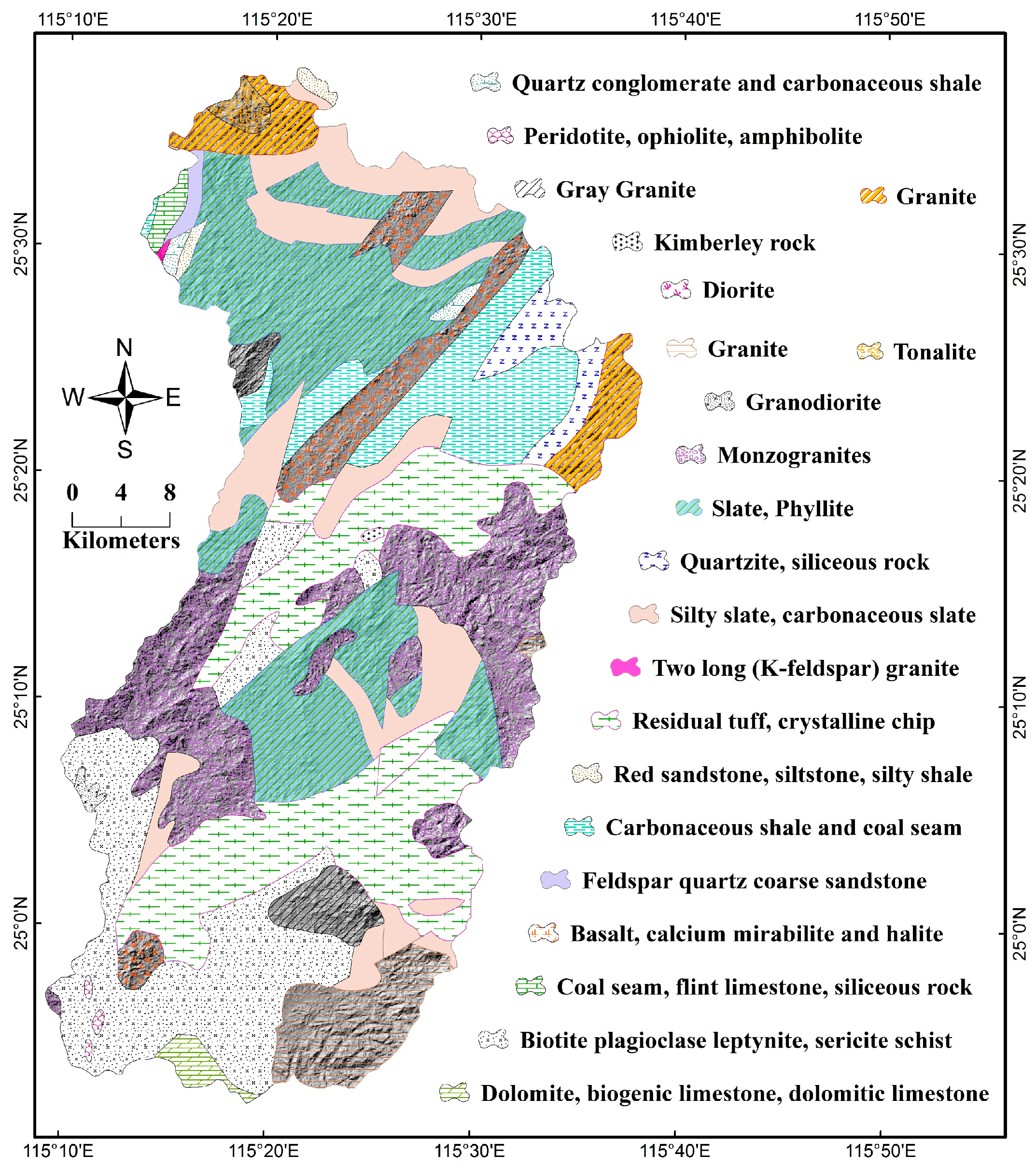
| No. | Unit Name | Lithology |
|---|---|---|
| A | Hutian group | Dolomite, biogenic limestone, dolomitic limestone |
| Two long (K-feldspar) granite | ||
| B | Zhong peng group | Red sandstone, siltstone, silty shale |
| Zi shan group, Yun shan group | Quartz conglomerate and carbonaceous shale | |
| C | Lu jing Unit | Kimberley rock |
| D | Lin shan group, Shui bei group | Carbonaceous shale and coal seam |
| Luo ao group | Feldspar quartz coarse sandstone | |
| Ge xianshan group, Xishan pai unit | Granite | |
| Linsha group, Yuexing group | Granite | |
| Yu tian group, Ji long group | Residual tuff; crystalline chip | |
| Long zhou unit | Diorite | |
| E | Shui jiang unit, Nankeng unit | Monzogranites |
| Gan zhou group, Zhou tian group | Basalt, calcium mirabilite and halite | |
| F | Yang jiaqiao group | Quartzite, siliceous rock |
| G | Da long group, Le ping group, Chang xing group | Coal seam, flint limestone, siliceous rock |
| Tao xi group | Biotite plagioclase leptynite, sericite schist | |
| H | Xia keng group | Granodiorite |
| I | Hu cheng unit | Tonalite |
| Gui keng unit, Shang you unit | Granite | |
| J | Le chang group | Slate, phyllite |
| He zi unit | Peridotite, ophiolite, amphibolite | |
| K | Bacun group, Niu jiaohe group | Silty slate, carbonaceous slate |
| Influencing Factors | Classes | No. of Pixels | No. of Landslide | SWARA Weight |
|---|---|---|---|---|
| Slope angle (degree) | <20.0 | 2656308 | 0 | 0.01 |
| 20.0–24.6 | 460317 | 116 | 0.11 | |
| 24.6–29.2 | 312393 | 95 | 0.14 | |
| 29.2–33.8 | 188594 | 46 | 0.11 | |
| 33.8–38.4 | 101643 | 35 | 0.16 | |
| 38.4–43.0 | 46703 | 16 | 0.16 | |
| 43.0–47.6 | 18080 | 4 | 0.10 | |
| >47.6 | 7394 | 3 | 0.19 | |
| Aspect | Flat | 1200 | 0 | 0.00 |
| North | 504881 | 12 | 0.03 | |
| Northeast | 433690 | 14 | 0.04 | |
| East | 479731 | 40 | 0.13 | |
| Southeast | 482847 | 70 | 0.23 | |
| South | 487601 | 97 | 0.30 | |
| Southwest | 431966 | 45 | 0.16 | |
| West | 480314 | 22 | 0.07 | |
| Northwest | 489202 | 15 | 0.04 | |
| Altitude (m) | 132–282 | 739706 | 4 | 0.01 |
| 282–432 | 1504606 | 75 | 0.06 | |
| 432–582 | 867013 | 148 | 0.22 | |
| 582–732 | 442338 | 39 | 0.11 | |
| 732–882 | 174022 | 35 | 0.26 | |
| 882–1032 | 55289 | 14 | 0.33 | |
| >1032 | 8458 | 0 | 0.00 | |
| Plan curvature | <−0.001 | 1791191 | 146 | 0.43 |
| (−0.001)–(0.001) | 171530 | 0 | 0.06 | |
| >0.001 | 1828711 | 169 | 0.51 | |
| Profile curvature | <−0.001 | 1835414 | 184 | 0.55 |
| (−0.001)–(0.001) | 33142 | 0 | 0.06 | |
| >0.001 | 1922876 | 131 | 0.39 | |
| SPI | 0–50 | 2957565 | 221 | 0.10 |
| 50–100 | 372535 | 48 | 0.16 | |
| 100–200 | 224014 | 25 | 0.14 | |
| 200–400 | 129200 | 10 | 0.11 | |
| 400–800 | 66033 | 8 | 0.15 | |
| 800–1000 | 12254 | 3 | 0.32 | |
| >1000 | 29831 | 0 | 0.01 | |
| STI | 0–10 | 2366364 | 90 | 0.04 |
| 10–20 | 797385 | 129 | 0.16 | |
| 20–30 | 300375 | 43 | 0.15 | |
| 30–40 | 129124 | 22 | 0.17 | |
| 40–50 | 67080 | 9 | 0.14 | |
| 50–60 | 39877 | 7 | 0.17 | |
| >60 | 91227 | 15 | 0.16 | |
| TWI | <3 | 444 | 0 | 0.01 |
| 3–5 | 1400515 | 200 | 0.61 | |
| 5–7 | 1708346 | 98 | 0.23 | |
| 7–9 | 514871 | 17 | 0.14 | |
| >9 | 167256 | 0 | 0.01 | |
| Lithology | A | 26836 | 0 | 0.01 |
| B | 27889 | 4 | 0.12 | |
| C | 2422 | 1 | 0.36 | |
| D | 1159282 | 126 | 0.09 | |
| E | 710946 | 32 | 0.04 | |
| F | 76373 | 6 | 0.06 | |
| G | 508520 | 41 | 0.07 | |
| H | 6902 | 0 | 0.01 | |
| I | 142618 | 21 | 0.13 | |
| J | 719372 | 61 | 0.07 | |
| K | 410272 | 23 | 0.05 | |
| Distance to faults (m) | 0–500 | 516832 | 60 | 0.21 |
| 500–1000 | 466826 | 37 | 0.15 | |
| 1000–1500 | 436370 | 44 | 0.19 | |
| 1500–2000 | 381470 | 43 | 0.20 | |
| 2000–2500 | 329017 | 26 | 0.15 | |
| >2500 | 1660917 | 105 | 0.11 | |
| Distance to rivers (m) | 0–150 | 1001961 | 47 | 0.07 |
| 150–300 | 799934 | 72 | 0.15 | |
| 300–450 | 703245 | 64 | 0.15 | |
| 450–600 | 543309 | 59 | 0.18 | |
| 600–750 | 388246 | 48 | 0.21 | |
| 750–900 | 220837 | 16 | 0.12 | |
| >900 | 220837 | 16 | 0.11 | |
| Land use | Bare | 656 | 0 | 0.00 |
| Forest | 1839583 | 243 | 0.53 | |
| Grass | 748647 | 45 | 0.24 | |
| Residential | 189281 | 5 | 0.11 | |
| Farmland | 994815 | 22 | 0.09 | |
| Water | 18450 | 0 | 0.00 | |
| NDVI | <(−0.05) | 110766 | 2 | 0.04 |
| (−0.05)–0.05 | 195838 | 7 | 0.07 | |
| 0.05–0.15 | 503739 | 18 | 0.07 | |
| 0.15–0.25 | 1185193 | 58 | 0.10 | |
| 0.25–0.35 | 1322962 | 141 | 0.20 | |
| 0.35–0.45 | 455283 | 88 | 0.40 | |
| >0.45 | 17651 | 1 | 0.12 | |
| Soil | ATc | 319882 | 2 | 0.02 |
| ACu | 1035811 | 153 | 0.54 | |
| ALh | 117324 | 6 | 0.19 | |
| ACh | 2290342 | 154 | 0.25 | |
| RGc | 28073 | 0 | 0.00 | |
| Rainfall (mm) | <1100 | 85055 | 0 | 0.01 |
| 1100–1200 | 427735 | 16 | 0.05 | |
| 1200–1300 | 1631694 | 74 | 0.06 | |
| 1300–1400 | 1040983 | 134 | 0.17 | |
| 1400–1500 | 433154 | 67 | 0.20 | |
| 1500–1600 | 78140 | 13 | 0.21 | |
| 1600–1700 | 38958 | 5 | 0.17 | |
| >1700 | 55713 | 6 | 0.14 |
| Influencing Factors | CIAV | Aj | wj = (W(j−1))/Aj | Weight wj/Sigma wj |
|---|---|---|---|---|
| Slope angle (o) | 1.000 | 1.000 | 0.105 | |
| Rainfall | 0.05 | 1.050 | 0.952 | 0.100 |
| Lithology | 0.1 | 1.100 | 0.866 | 0.091 |
| Soil | 0.06 | 1.060 | 0.817 | 0.086 |
| Land use | 0.06 | 1.060 | 0.771 | 0.081 |
| NDVI | 0.07 | 1.070 | 0.720 | 0.076 |
| Distance to Rivers (m) | 0.07 | 1.070 | 0.673 | 0.071 |
| Distance to faults (m) | 0.03 | 1.030 | 0.653 | 0.069 |
| TWI | 0.05 | 1.050 | 0.622 | 0.066 |
| SPI | 0.08 | 1.080 | 0.576 | 0.061 |
| Altitude | 0.1 | 1.100 | 0.524 | 0.055 |
| STI | 0.1 | 1.100 | 0.476 | 0.050 |
| Aspect | 0.3 | 1.300 | 0.366 | 0.039 |
| Profile curvature | 0.3 | 1.300 | 0.282 | 0.030 |
| Plan curvature | 0.5 | 1.500 | 0.188 | 0.020 |
© 2019 by the authors. Licensee MDPI, Basel, Switzerland. This article is an open access article distributed under the terms and conditions of the Creative Commons Attribution (CC BY) license (http://creativecommons.org/licenses/by/4.0/).
Share and Cite
Chen, W.; Hong, H.; Panahi, M.; Shahabi, H.; Wang, Y.; Shirzadi, A.; Pirasteh, S.; Alesheikh, A.A.; Khosravi, K.; Panahi, S.; et al. Spatial Prediction of Landslide Susceptibility Using GIS-Based Data Mining Techniques of ANFIS with Whale Optimization Algorithm (WOA) and Grey Wolf Optimizer (GWO). Appl. Sci. 2019, 9, 3755. https://doi.org/10.3390/app9183755
Chen W, Hong H, Panahi M, Shahabi H, Wang Y, Shirzadi A, Pirasteh S, Alesheikh AA, Khosravi K, Panahi S, et al. Spatial Prediction of Landslide Susceptibility Using GIS-Based Data Mining Techniques of ANFIS with Whale Optimization Algorithm (WOA) and Grey Wolf Optimizer (GWO). Applied Sciences. 2019; 9(18):3755. https://doi.org/10.3390/app9183755
Chicago/Turabian StyleChen, Wei, Haoyuan Hong, Mahdi Panahi, Himan Shahabi, Yi Wang, Ataollah Shirzadi, Saied Pirasteh, Ali Asghar Alesheikh, Khabat Khosravi, Somayeh Panahi, and et al. 2019. "Spatial Prediction of Landslide Susceptibility Using GIS-Based Data Mining Techniques of ANFIS with Whale Optimization Algorithm (WOA) and Grey Wolf Optimizer (GWO)" Applied Sciences 9, no. 18: 3755. https://doi.org/10.3390/app9183755
APA StyleChen, W., Hong, H., Panahi, M., Shahabi, H., Wang, Y., Shirzadi, A., Pirasteh, S., Alesheikh, A. A., Khosravi, K., Panahi, S., Rezaie, F., Li, S., Jaafari, A., Bui, D. T., & Bin Ahmad, B. (2019). Spatial Prediction of Landslide Susceptibility Using GIS-Based Data Mining Techniques of ANFIS with Whale Optimization Algorithm (WOA) and Grey Wolf Optimizer (GWO). Applied Sciences, 9(18), 3755. https://doi.org/10.3390/app9183755